Multi-Channel Wireless Traffic Sensing and
Characterization for Cognitive Networking
Bheemarjuna Reddy Tamma
∗, Nicola Baldo
†, B. S. Manoj
∗, and Ramesh R Rao
∗∗
California Institute for Telecommunications and Information Technology – UC San Diego, USA
†Centre Tecnol`ogic de Telecomunicacions de Catalunya – Barcelona, Spain
{
btamma,bsmanoj,rrao
}
@ucsd.edu, [email protected]
Abstract— Traffic sensing and characterization is an important building block of cognitive networking systems; however, it is very challenging in multi-channel multi-radio wireless networks. The contributions of this paper include the following: (i) a discussion of packet sampling for traffic sensing in multi-channel wireless networks, (ii) a comparison of various time-based sampling strategies using the Kullback-Leibler Divergence (KLD) measure, (iii) a study of the effect of the sampling parameters on the accuracy of the sampling strategies, (iv) the proposal of a new metric (Traffic Intensity) which estimates the busyness of channels by taking into consideration not only the successfully received packets but also corrupt or broken packets, and (v) some preliminary results on the characterization of a campus 802.11 network environment in a spatio-temporal fashion.
I. INTRODUCTION
A cognitive network is defined as a network with a cognitive controller that can perceive current network conditions, and then plan, decide, and act on those conditions [1]. Hence the cognitive controller needs to gather, compact, analyze, and reposit large amounts of wireless network traffic across several dimensions such as space, time, and frequency to characterize the wireless environment and the state of the network. However, in most of the existing studies on the characterization of wireless LANs, measurements have been conducted on wired portion of the network [2]. While it is easier to make consistent measurements in wired portion of the network, such measurements cannot monitor the actual 802.11 frames spread across multiple channels and hence fail to observe the significant vagaries present in wireless spectrum. In [3] and [4] the authors proposed wireless monitoring systems for enterprise 802.11b/g networks. The proposed monitoring system consists of a set of wireless traffic sen-sors, each one equipped with one or more wireless network interface cards (NICs) that are configured on one of the orthogonal channels (1, 6, and 11) to monitor all the traffic in those channels; traces obtained from multiple sensors are then merged to construct a global view of network activity, from which one can extract characteristics like application workloads, user session durations, user mobility patterns, and temporal network usage patterns. The cognitive networking paradigm, however, requires a characterization of the wireless network traffic present in each channel in a spatio-temporal
This work was supported by NSF sponsored projects, at University of California San Diego, Rescue, CogNet, and Responsphere (award numbers: 0331690, 0650048, and 0403433, respectively).
fashion. Such kind of characterization helps the network to tailor its optimization criteria to different network elements present in the system. To address this issue, we employ traffic sensors that monitor traffic on all wireless channels, and furthermore the cognitive controller does not merge the traces, but stores them across three dimensions: space (location of traffic sensor), time, and frequency (channel).
The traffic in wireless LANs is spread across a number of channels, whereas a single wireless NIC can typically monitor only one channel at a time. The 802.11b/g-based wireless networks operate on ISM band and have 11 chan-nels. Even though orthogonal channels are typically used for configuring APs, in some cases (e.g., non-802.11 sources such as Bluetooth, microwave ovens, and noise rendering an orthogonal channel useless) other channels are also being used in the configuration of APs. In some scenarios APs belong to different wireless LANs co-exist on the same channel and compete for radio resources in the same geographic region. To characterize traffic in such network environments, the wireless monitoring system should have the capability of monitoring all wireless channels in a spatio-temporal fashion. In order to characterize wireless traffic on all channels, the traffic sensor has either to have a dedicated wireless NIC per channel in order to measure all the traffic in that channel, or to switch a single wireless interface across all the channels in a round-robin fashion, thus measuring a fraction of traffic on each channel. In the first case, the sensor device would be very complex due to the large number of channels being used, and moreover the transmission, storage, and analysis of the captured packets from a large number of simultaneous chan-nels could be problematic. Therefore, such a multi-interface complete capture solution would be very expensive and would scale poorly to large scale multi-channel wireless network environments. The multi-channel traffic sampling scheme is therefore essential.
As a scalable means of monitoring network traffic, traffic sampling has attracted much attention from the industrial and research communities. Sampling is a form of passive traffic measurement, in which not all packets are measured, but only a fraction of them, which is selected based on the sampling method and parameters associated with the sampling process. Based on the sampling algorithm, there are three main classes of sampling methods: systematic sampling, stratified random sampling, and simple random sampling [5]. In systematic
sampling, packets are selected deterministically from each sampling interval or period. Stratified random sampling in-volves selecting packets randomly from each sampling inter-val, whereas in the case of simple random sampling packets are selected randomly from the parent population.
Based on the type of trigger used to start the packet capture, sampling methods can be broadly classified into count-based and time-based sampling [6]. In count-based sampling, the packet count triggers the start of a sampling interval or sampling period. Here, the sampling period is defined in terms of the number of packets. The sampling duration or length defines number of packets selected for inclusion in the sample from each sampling interval. An example of systematic count-based sampling is to select every nth packet in the packet stream. We note that implementing a count-based traffic sampling method is very expensive in a multi-channel wireless network environment, as we do not know in advance at what times packets will appear on the channel and packet arrival rates vary across the channels, and therefore it requires one dedicated wireless NIC to sense each channel.
In time-based sampling, the sampling period is defined as a time interval. However, the sampling duration can either be timer-driven or count-driven. Hence time-based sampling can be further classified into timer-driven time-based sampling and count-driven time-based sampling. An example of systematic timer-driven time-based sampling is to capture all packets arriving in the first 1 s of every 11 s. An example of systematic count-driven time-based sampling is to sample one packet every 11 s. For both examples sampling period or cycle is 11 s, but sampling durations or lengths are 1 s and one packet, respectively. The various time-based sampling schemes are summarized in Table I. The time-based sampling methods seem to offer a cost-effective and scalable solution by reducing the cost of resources for characterizing wireless traffic. For example, the use of time-based sampling enable us to make use of a single wireless NIC to sample multiple channels. However, we need to determine which one of these sampling strategies provides us with better sampling accuracy under what combination of parameters.
TABLE I
TIME-BASEDSAMPLINGSCHEMES Sampling Method Sampling Algorithm Trigger Type
SCT Systematic Count-driven Time-based STT Systematic Timer-driven Time-based SRCT Stratified Random Count-driven Time-based SRTT Stratified Random Timer-driven Time-based
II. Related Work
Most of the existing studies on characterization of wireless traffic (see [2], [3], [4] and the references in them), relied upon wired monitoring and/or the use of SNMP statistics, and hence failed to characterize the wireless spectrum in a spatio-temporal fashion. Some work which employed wireless traffic sensors focused on the merging of traces and the character-ization of global network activity [2], [3], [4]. However the cognitive networking paradigm requires the characterization of
the traffic on all channels in a spatio-temporal fashion. Hence the wireless monitoring system should have the capability to sample a fraction of the traffic from all wireless channels. In [7], the authors studied the sampling accuracy of time and count-based methods for both random and systematic periods of sampling for wired wide area network traffic. However, they only studied count-driven time-based sampling. Their result mainly pointed to the inappropriateness of using the count-driven time-based techniques because they do not perform as well as the count-based ones. Desphande et al. [8] proposed two methods for channel-based sampling in IEEE 802.11b/g networks. However, the effect of sampling parameters on the accuracy of sampling, which is one of the most important aspects, is not studied in their paper. Hence, we would like to study the accuracy of Time-based sampling schemes by varying the sampling period and sampling durations for traffic sensing in multi-channel wireless networks. Then we present some preliminary results on the characterization of a campus 802.11 network environment in a spatio-temporal fashion.
III. ACCURACY OFSAMPLING
To measure and compare the performances of various sam-pling methods, we need a metric to measure how close the distributions given by the sampling methods are, compared to the actual distributions of the parent populations. We use a popular statistical measure that quantifies the distance, or relative entropy, between two probability distributions.
Let p(x) denote the probability mass function for the distribution of the parent population packet trace. The prob-ability mass function defines the probprob-ability that the traffic metric under study (e.g., packet size and RSSI) lies in certain intervals. Let q(x) denote probability mass function for the distribution of the sampled packet trace obtained by applying one of the sampling methods. The normalized Kullback-Leibler Divergence (NKLD) [9] is defined as
N KLD(p(x)||q(x)) = KLD(p(x)||q(x)) H(p(X)) (1) where KLD(p(x)||q(x)) = x∈χ p(x)logp(x) q(x) and H(p(X)) = x∈χ p(x)log 1 p(x)
H(p(X)) is the entropy of the random variable X with distribution p(X). The KLD is zero when the distributions are identical and strictly positive otherwise. The calculation of NKLD measure requires the selection of a set of intervals (χ) for the traffic metric distribution under investigation. In our experiments, for each traffic metric distribution we choose
χ in such a way that each interval contains at least 1% of data from the population data set. For example, in case of packet size distribution we start from the lowest packet size value found in the population data set and increase the value until we get at least 1% of data to obtain the boundary of the first interval.Then beginning with the boundary of the first interval, we repeat above procedure to obtain the boundary of the second interval, and so on. Once intervals are known, it is
straight forward to obtain the probability mass functions for the population packet trace and sampled packet traces.
IV. OUREXPERIMENTAL SETUP
All of our wireless traffic monitoring activity took place within the University of California San Diego division of CALIT2, a large six-story building. Among production APs located on 4th and 6th floors, we have deployed 11 CalNodes (wireless traffic sensor devices) [6], [10]. Each CalNode consists of a Soekris net4521 system board with one Ubiquity 802.11 a/b/g wireless NIC configured in monitor mode to capture all 802.11 packets in the air. Each CalNode runs on Voyage Linux with kernel 2.6.x and uses the open source MadWiFi driver. Each CalNode is connected to the campus intranet via one of the Ethernet interfaces to transfer capture packets to the CogNet repository. To reduce the storage cost, we configuredtcpdumpto capture only the first 250 bytes (144 bytes for Prism monitoring header) of each sampled packet. Prism header and other protocol header fields that are extracted from the sampled packets are stored in a MySQL database. In addition to traffic samples, we gather additional statistics like the number of CRC errors (i.e., receptions failed due to bad CRC in the MAC trailer) and PHY errors (receptions failed due to the CRC failure on the PLCP header) with the help of athstatstool available in MadWIFI driver.
To get samples at different granularities for various Time-based sampling schemes and measure their sampling accuracy using the NKLD measure, we need population (i.e.,complete) packet traces. Therefore we configured a couple of CalNodes to do continuous packet capture on one particular orthogonal channel for four weeks. We treat these traces as our parent population data sets and generate different sample traces by varying sampling duration and sampling period for various Time-based sampling methods.
V. PERFORMANCERESULTS
In this study our target per-packet traffic distributions are inter-arrival times, packet sizes, and RSSIs. For each of the sampling schemes, we generate samples at different level of granularity. In the graphs all performance results are shown with 95% confidence intervals.
A. Comparison of Sampling Schemes
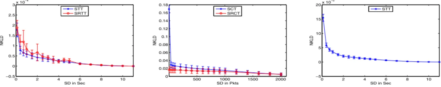
Figure 1 shows the NKLD measures for the distribution of the packet size metric calculated from various samples obtained from STT and SRTT sampling schemes. In this experiment, we kept the Sampling Period (SP) constant at 11 s and varied the Sampling Duration (SD) from 100 ms to 11 s to obtain various samples from the parent population packet size trace. As SD increases (i.e., the sample size increases) the values of NKLD gradually decrease. Overall, we see a small divergence between the population packet size trace and sampled packet size traces obtained from STT and SRTT schemes. In addition, when the SD goes beyond 1 s, the variation in the NKLD decreases. In other words, even samples generated with a SD of 1 s are closely matching
the distribution of parent population. From the figures we can also observe that the performance of the STT and the SRTT sampling schemes are almost identical. However, as SRTT requires the generation of pseudo-random numbers, it is more expensive to implement it in real sampling systems.
In Fig. 2 we show the NKLD measures of count-driven time-based schemes, SCT and SRCT. For these sampling schemes SD is defined as the number of packets to capture for inclusion in the sample during SP. As shown in the figure, the performance of SCT and SRCT schemes is almost identical. However, when we compare these schemes against the timer-driven time-based schemes (STT and SRTT), the NKLD measures are significantly lower for the timer-driven time-based schemes than for the count-driven time-time-based sampling schemes (SCT and SRCT). This is because in count-driven time-based schemes the sample size is fixed (as SD is defined in terms of packet count) and does not grow linearly with the traffic load in the network, while in the case of the STT and SRTT schemes sample size grows proportionally to the traffic load, as SD is defined as a time interval. From the above results, we conclude that the STT sampling scheme is the best sampling strategy in terms of sampling accuracy and ease of implementation in real systems. We now employ STT and compute NKLD measures for samples obtained from the population of packet inter-arrival times, packet data rates, and packet RSSI traces. Figs. 3 and 4 show their corresponding NKLD scores. Comparing these figures with Fig. 1 we can observe that the inter-arrival time distribution has the lowest NKLD values. Out of the three traffic metrics studied, the samples of packet RSSI exhibit higher divergence from the population packet trace. Since the maximum divergence is still very small, we can configure the monitoring nodes to perform STT sampling to accurately sense all the traffic metrics in multi-channel wireless network environments.
B. Effect of the Sampling Period
In these experiments we kept SD constant at 1 s and compute the NKLD from the samples obtained using the STT sampling scheme by varying SP from 1 s to 32 s. Figs. 5 and 6 show the corresponding NKLD values for the traffic metrics under study. The results for the packet RSSI metric have been omitted due to space constraints. As expected, for all the traffic metrics the NKLD increases when SP increases due to decrease in sample size. We can also observe that the packet inter-arrival time distribution is having the lowest divergence values. We also conducted similar experiments by varying channel number for four weeks in our campus; the results are very similar to what we presented in this paper. In order to reduce the cost of wireless traffic characterization, we would like to reduce the value of SD and increase the value of SP to maximum extents without sacrificing sampling accuracy. Even though there are 11 channels to be monitored for traffic in IEEE 802.11b/g spectrum, when we employ timer-driven time-based sampling with sampling parameters SD=1 s and SP=11 s, one wireless interface would be sufficient for sensing all the channels.
0 2 4 6 8 10 −0.5 0 0.5 1 1.5 2 2.5 3x 10 −4 SD in Sec NKLD STT SRTT
Fig. 1. NKLD of STT and SRTT schemes vs SD for packet size distribution.
500 1000 1500 2000 0 0.02 0.04 0.06 0.08 0.1 0.12 0.14 0.16 0.18 SD in Pkts NKLD SCT SRCT
Fig. 2. NKLD of SCT and SRCT schemes vs SD for packet size distribution.
0 2 4 6 8 10 −5 0 5 10 15 20x 10 −5 SD in Sec NKLD STT
Fig. 3. NKLD of STT scheme vs SD for inter-arrival time distribution.
0 2 4 6 8 10 0 0.5 1 1.5 2 2.5 3 3.5x 10 −4 SD in Sec NKLD STT
Fig. 4. NKLD of STT scheme vs SD for packet RSSI distribution. 5 10 15 20 25 30 −1 0 1 2 3 4 5 6x 10 −4 SP in Sec NKLD STT
Fig. 5. NKLD of STT scheme vs SP for packet size distribution. 5 10 15 20 25 30 −5 0 5 10 15 20x 10 −5 SP in Sec NKLD STT
Fig. 6. NKLD of STT scheme vs SP for inter-arrival time distribution.
C. Historical Traffic Statistics
Though metrics like the packet rate (packets per second) and the traffic load (bits per second) indicate the busyness of wireless channels to some extent, they fail to quantify the utilization of radio resources in a clear and compact fashion. With this respect, a more representative metric is the Traffic Intensity (TI), defined as the fraction of time in which the channel is occupied. We now present an effective strategy for estimating each channel’s TI from the sampled packet traces. LetKdenote the number of packets sampled in an interval of duration T, and letdi be the transmission duration of the
ithpacket. Then TI in the interval being considered is T IT:
T IT =
i=K i=1 di
T (2)
In the case of sampled traffic traces obtained from the STT sampling scheme with SD=1 s and SP=11 s, the per-hour calculation of TI in given channel hasT=60*60/11=327.27 s. As per Eqn (2), TI takes into consideration only the channel re-sources consumed by successfully received packets. However, corrupt or broken packets also consume a significant amount of channel resources. We use the average transmission duration of successfully received packets in a given time interval to estimate the TI contribution provided by CRC error packets. Furthermore, we use 20μs (time taken to transmit PLCP header at the basic PHY rate in 802.11b/g cards) as the duration of the contribution to TI given by PHY errors. Let CRCT and
P HYT denote CRC and PHY error counts in time intervalT.
Then we define T IERROR as
T IERRORT = ( i=K i=1 di K + 20µs)·CRCT+ 20µs·P HYT T (3)
The total TI for a time intervalT is obtained as the sum of
T IT andT IERRORT, given respectively by Eqns (2) and (3). Unlike other metrics, TI metric is able to estimate the busyness of channels by taking into consideration both successfully received packets and corrupt or broken packets. This feature provides us with an effective way of estimating the amount of channel resources consumed by both 802.11 transmissions on adjacent channels as well as by non-802.11 interferers.
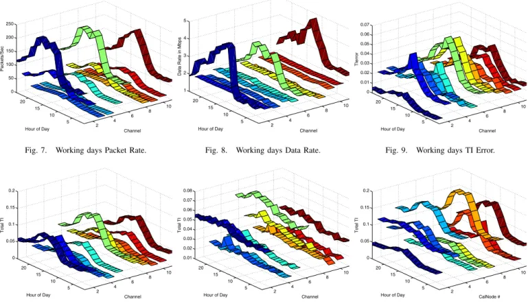
We implemented the STT sampling scheme in all our CalNodes with SD=1 s and SP=11 s and collected samples for all days in August 2008. Due to space constraints, here we only show a few of the estimated population traffic statistics for one traffic sensor. Figs. 7 and 8 show mean packet rates (fps) and data rates (bps) during normal working days1 for all
11 channels. Even though orthogonal channels (1, 6, and 11) contain higher traffic due to presence of production network APs, other channels also face traffic to a certain extent due to the leakage of wireless signals (especially those transmitted at basic rate of 1 Mbps, as evident from Fig. 8) into adjacent channels. It can also be observed from Fig. 7 that leakage of packets is more into immediate adjacent channels: 2, 5, 7, and 10. From above figures, one could come to a conclusion that the traffic is very similar across the orthogonal channels. However this is not true in terms of traffic intensity metric, as shown in Figs. 9, 10, because radio resource consumption is different in those channels. Since wireless signals from or-thogonal channels leak into adjacent channels, those channels experience a lot of CRC and PHY errors, and actually face a high consumption of radio resources (estimated usingTIError metric) as shown in Fig. 9. Fig. 10 shows the mean total TI 1Monday to Friday, for a total of 21 working days in the observation period
2 4 6 8 10 5 10 15 20 0 50 100 150 200 250 Channel Hour of Day Packets/Sec
Fig. 7. Working days Packet Rate.
2 4 6 8 10 5 10 15 20 1 2 3 4 5 Channel Hour of Day Data Rate in Mbps
Fig. 8. Working days Data Rate.
2 4 6 8 10 5 10 15 20 0 0.01 0.02 0.03 0.04 0.05 0.06 0.07 Channel Hour of Day TIerror
Fig. 9. Working days TI Error.
2 4 6 8 10 5 10 15 20 0 0.05 0.1 0.15 0.2 Channel Hour of Day Total TI
Fig. 10. Working days Total TI.
2 4 6 8 10 5 10 15 20 0.01 0.02 0.03 0.04 0.05 0.06 0.07 0.08 Channel Hour of Day Total TI
Fig. 11. Holidays Total TI.
2 4 6 8 10 5 10 15 20 0 0.05 0.1 0.15 0.2 CalNode # Hour of Day Total TI
Fig. 12. Working days Total TI on Channel 6 across all CalNodes.
(including both the contribution due to successfully received packets and TI due to corrupt or broken packets) during working days for all 11 channels. It is to observed that traffic is high in Channel 6 compared to other two orthogonal channels. Furthermore, there is a significant difference in traffic patterns of working days and holidays as shown in Fig. 11. While the mean traffic increases during business hours of working days, it stays pretty much constant for the whole day during non-working days2. It is to be noted that traffic is non zero
for non-working hours as the APs of the campus production network always send periodic beacons.
We now take Channel 6 as a representative channel and plot variation of Total TI in a spatio-temporal fashion in Fig. 12. CalNodes 1-7 and 8-11 are deployed on the 6th and 4th floors of CALIT2 building, respectively. From the figure we can observe that Total TI is also varying in spatial dimension and it is highest at CalNode 8 deployed on the 4th floor.
VI. CONCLUSIONS
In this paper, we studied the accuracy of various time-based sampling schemes and found that the Systematic Timer-driven Time-based (STT) sampling strategy is the ideal sampling strategy for traffic sensing and characterization in multi-channel wireless networks. Our future work includes the design of a Cognitive network controller which can use the 2Saturday and Sunday, for a total of 10 days in the observation period. We
note that there are no public holidays in the observation period.
sampling strategies and traffic statistics that we discussed to learn the channel conditions and the status of the network, and finally to select the most desirable network configuration.
REFERENCES
[1] R. W. Thomas, D. H. Friend, L. A DaSilva, and A. B. MacKenzie, “Cognitive Networks: Adaptation and Learning to Achieve End-to-end Performance Objectives”,IEEE Communications Magazine, vol. 44, no. 12, pp. 51-57, December 2006.
[2] Magdalena Balazinska and Paul Castro, ”Characterizing Mobility and Network Usage in a Corporate Wireless Local-Area Network“,ACM Mobisys, pp. 303-316, 2003.
[3] Jihwang Yeo, Moustafa Youssef, Tristan Henderson, and Ashok Agrawala, ”An Accurate Technique for Measuring the Wireless Side of Wireless Networks“,Workshop on Wireless Traffic Measurements and Modeling, pp. 13-18, 2005.
[4] Yu-Chung Cheng, John Bellardo, P´eter Benk¨o, Alex C. Snoeren, Geoffrey M. Voelker, and Stefan Savage, ”Jigsaw: Solving the Puzzle of Enterprise 802.11 Analysis“,SIGCOMM Comput. Commun. Rev., vol. 36, no. 4, pp. 36-50, 2006.
[5] N. Duffield, “Sampling for Passive Internet Measurement: A Review”,
Statistical Science, vol. 19, no. 3, pp. 472-498, 2004.
[6] Bheemarjuna R. Tamma, B.S. Manoj, and Ramesh Rao, ”Time-based Sampling Strategies for Multi-channel Wireless Traffic Characterization in Tactical Cognitive Networks“,in Proc. of IEEE MILCOM, pp. 1-7, November 2008.
[7] K. C. Claffy, G. C. Polyzos, and H.-W. Braun, “Application of Sam-pling Methodologies to Network Traffic Characterization”,Computer Communication Review, vol. 23, no. 4, pp. 194-203, October 1993. [8] U. Deshpande, T. Henderson, and D. Kotz, “Channel Sampling
Strate-gies for Monitoring Wireless Networks”,in Proc. of WiOpt, pp. 1-7, April 2006.
[9] S. Kullback, “Information Theory and Statistics”, John Wiley and Sons Inc., New York, 1959.