ISSN Online: 2153-120X ISSN Print: 2153-1196
DOI: 10.4236/jmp.2019.104027 Mar. 19, 2019 423 Journal of Modern Physics
Quantum Interference without Quantum
Mechanics
Arend Niehaus
*Utrecht University, Utrecht, The Netherlands
Abstract
A recently proposed model of the Dirac electron, which has been shown to describe several observed properties of the particle correctly, is in the present paper shown to be also able to explain quantum interference by classical probabilities. According to this model, the electron is not point-like, but ra-ther an “entity with structure”, formed by a fast periodic motion of a “light-like object”, whose momentum (p) causes the angular momentum responsible for the spin, and whose energy (E = pc) is equal to the energy of the electron, mc2. A qualitative description of the model is given, together with the
quan-titative formulae that allow to discuss interference. Applied to the experi-mental situation of the “two-slit” experiment, the formulae yield the same time dependence of the detection probability as the quantum mechanical treatment, and hence the same interference pattern. In contrast to quantum mechanics, the pattern is due to “particle interference” rather than to “wave interference”. No wave-particle paradox arises. The merits of the model are summarized, and its physical content discussed.
Keywords
Interpretation of Quantum Mechanics, Quantum Interference, Classical Probability
1. Introduction
Quantum mechanics treats the electron as a point-like particle having a certain mass, but no structure. To describe observed phenomena correctly, it ascribes certain other properties to the particle, for instance spin, and a wavelike nature, which are “non-classical”, and cannot be “derived” (e.g. [1]). The validity of the theory is unquestioned; however, its interpretation is still subject of debate (see, f.i., [2]), because the “quantum world” it creates contains numerous well known paradoxes.
*Retired Professor of Physics. How to cite this paper: Niehaus, A. (2019)
Quantum Interference without Quantum Mechanics. Journal of Modern Physics, 10, 423-431.
https://doi.org/10.4236/jmp.2019.104027
Received: February 9, 2019 Accepted: March 16, 2019 Published: March 19, 2019
Copyright © 2019 by author(s) and Scientific Research Publishing Inc. This work is licensed under the Creative Commons Attribution International License (CC BY 4.0).
http://creativecommons.org/licenses/by/4.0/
DOI: 10.4236/jmp.2019.104027 424 Journal of Modern Physics There have been attempts to escape interpretational problems by supposing that the electron, and possibly other elementary particles also, do have an inter-nal structure that possibly could explain their properties. Especially, the fact that a so called “Zitterbewegung (ZBW)” [3] is one of the properties arising from the relativistic quantum theoretical treatment of the free electron, has led to the proposal of a dynamic substructure [4] [5] [6]. Typical time scale for such a structure would be the very short period (τ) of the (ZBW):
τ = 2π/ωZBW with ωZBW = 2c/L0, leading to τ = 2πL0 /2c ≈ 4∙10−21 s.
Theoretical analyses have indeed shown that the spin, arising in the Dirac theory, can be related to a motion; however, an extended (ZBW), not predicted by the Dirac theory, would be necessary to explain the properties of the electron
[6]. Also models of the electron, based on the (ZBW), have been proposed [7] [8]. For a recent discussion we refer to [9].
The model to be used in this paper, is also based on the assumption of a (ZBW). But the new aspect is that, the (ZBW) is not ascribed to the electron, but rather to a light-like object that possesses momentum and energy, and establish-es the electron by its periodic motion around a point in space. The model has been developed in two recent publications [10][11]1 of the present author, and
has been shown to explain the properties like spin, magnetic moment, and mass, of the electron. In the present paper it will be shown to be also able to explain quantum interference using classical probabilities. First, we give a short qualita-tive description of the model.
Starting from the assumption that spin is caused by orbital motion due to an extended (ZBW), a probability distribution of orientation and value of an in-stantaneous orbital angular momentum is designed, which describes spin and spin measurements in accordance with experiment. Under the assumption that the “object” that causes the angular momenta is “light-like”, with momentum (p = ħ/L), probability distributions for orientation and length of the instantaneous position vector of the “light-like object”, which we will call “quantum”, are de-rived from the angular distributions. The instantaneous positions of the quan-tum turn out to lie on a torus around a fixed point, the torus radius (Rt) being
equal to the radius of the circle (Rc) the torus axis forms around the fixed point:
Rt = Rc = (L/2). This special Torus is a so called Clifford Torus. The relation
be-tween instantaneous position vector (r) of the quantum, its instantaneous mo-mentum (p), and the resulting instantaneous angular momentum vector (I = r × p) is depicted in Figure 1.
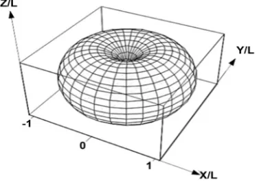
The Torus, on whose surface the instantaneous positions of the quantum are located, is shown in Figure 2.
In Cartesian coordinates the position vector is given by
(
)
{
2( ) ( )
2( ) ( )
( ) ( )
}
, , cos cos , cos sin , sin cos
r x y z =L θ ϕ θ ϕ θ θ (1)
The idea is now, to describe the distributions in terms of the extended ZBW of
1Erroneously, the labels (a) and (b) of the two figures in Figure 3 were interchanged in the final
DOI: 10.4236/jmp.2019.104027 425 Journal of Modern Physics Figure 1. Relation between the following instantaneous
vectors, 1) momentum (p) of the quantum, 2) its position (r), and 3) of the resulting angular momentum I = r × p. Equal population of the circle around the point Ph by the quantum, together with cylindrical symmetry around the Z-axis, lead to the required angular distribution I(θ) = (h/2π)cos(θ), which explains spin and spin measurements correctly (see Ref. [10]).
Figure 2. The instantaneous positions of the quan-tum are located on the surface of a Clifford Torus. The torus radius (Rt) is equal to the radius of the cir-cle (Rc) the torus axis forms around the fixed point: Rt = Rc = L/2.
the quantum. To obtain a motion of the quantum on the torus surface, we relate the angles
( )
θ φ
,
as; ;
2
t
pt t p n t
ω
ϕ ω θ= = ω = ω
(2)
The parameter (t) is taken to be proper time, so that (ωp, ωt) are frequencies,
[image:3.595.281.470.420.552.2]DOI: 10.4236/jmp.2019.104027 426 Journal of Modern Physics torus. From (1) we get:
(
)
2( )
2( )
sin( )
, , , cos cos , cos sin ,
2 2 2
t
t t
p p
t r x y z t = L ω t ω t ω t ω t ω
(3)
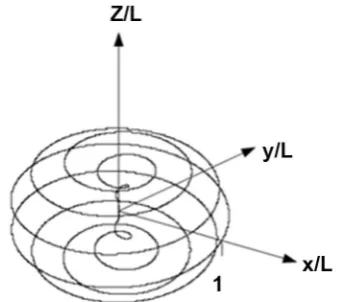
As an example, we show in Figure 3 the path for the case n = 10 as calculated with (3).
Properties of the “entity” obtained using relation (3) as averages over an ob-servation time, approach definite values after times sufficiently long compared to the period τ = 4π/ωt. If (L) is taken to be the reduced Compton wavelength L
= ħ/mc, with (m) the relativistic mass of the particle described, such values are, for instance, spin = ħ/2, and the correct magnetic moment = ħe/(2m0). We stress
that the value of the number (n) has no influence on the general situation de-scribed so far.
We identify the “entity”, if it is observed with a sufficiently low time-resolution, with the particle described. Then, the center of the torus is the position of the particle, and due to the dynamical origin of its torus-structure, it has its estab-lished properties.
In this paper we attempt to describe the property “wave nature” of moving particles. It becomes observable by the phenomenon interference, for instance in the two-slit experiment. Therefore, the velocity (v) is introduced into the model represented so far by relation (3). Assuming a velocity in Z-direction, this is done in the following way:
1) The coordinate (z) is replaced by
(
z vt
+
)
; 2)(
2)
1 2 0 1L=L −
β
with v cβ = ; 3)
ω
p =2c L0 so thatω
p becomes the ZBW-frequency arising inthe Dirac theory.
The velocity component at the torus axis (at point Ph in Figure 1) in the X-Y
plane thus becomes
(
2)
1 22 1
pL c
ω
= −β
, and the velocity component in [image:4.595.292.464.502.653.2]Z-direction is (βc), resulting in a constant tangential speed (c) at the torus axis,
DOI: 10.4236/jmp.2019.104027 427 Journal of Modern Physics independent of (v), as required. The ratio of the frequencies becomes:
(
2)
1 21
p t n
ω ω
= = −β
β
, so that(
2)
1 2 1 1 nβ
= + .The complete model for the case of a velocity (v = βc) in Z-direction may thus be represented by the modified relation (3) as follows:
(
)
( )
( )
( )
2 2 0 0 , , , , sincos cos , cos sin ,
2 2 2
t
t t
p p
r x y z t
t ct
L n t t t t
nL β
ω
ω ω
β ω ω
= +
(
)
1 2 2 00 0
2
; p ; t p; 1
c
L n
m c L n
ω
ω ω β β
= ħ = = = − ; (4)
The model is completely general and contains no free parameters. In this pa-per we will demonstrate, in which way it describes observed interference phe-nomena of electrons correctly. As example we discuss the two slit experiment in paragraph (2).
2. Interference
First we show in Figure 4 a 3D-parametric plot of the path of the quantum dur-ing a time span of 2.5 periods
(
τ
=
4
π ω
t)
for the case n = 10, as calculatedusing relation (4).
In order to treat interference in the two-slit experiment, we need the velocity of the quantum in Z-direction (vq). As calculated using (4), this velocity is given by
(
)
2 2
2 cos 2 cos
2
t
DB
vq v ω = v ω t
= (5)
where, according to the definition of the Torus frequency given in (4), ωDB is the
De Broglie frequency defined as ωDB = c/LDB= c mv/ħ.
For the case of many particles starting with a different phase (φ) from a cer-tain position in Z-direction, there arises a constant current of quanta in Z-direction, which is obtained by integration over (φ). Assuming equal proba-bility (1/2π) for different phases, the current becomes
( )
2π 2(
)
0 1
2 cos d
2π DB
I t = v
ω
t+ϕ ϕ
=v
∫
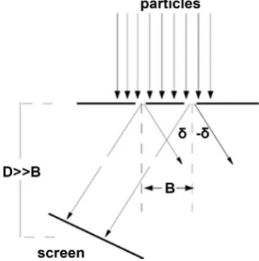
(6)Let us now consider the normal two-slit situation in the context of the model, where diffracted particles from the two narrow slits separated by distance (B) form currents into certain directions behind the slits, and hit the surface of a screen that is oriented perpendicular to the currents and positioned at a distance large compared to the distance between the two slits (see Figure 5).
DOI: 10.4236/jmp.2019.104027 428 Journal of Modern Physics Figure 4. Traces from left to right: 1), A parametric 3D plot of the positions in real space of the quantum (in units of L) during the first 2.5 periods of the (EZBW), for the case n = 10. 2), Path of the quan-tum during one period, starting 1.3 periods after (t = 0). 3), Path of the point (Ph) on the torus axis (see Figure 1) during the first pe-riod. Its tangential speed is (c) (see text). Progress of the “entity” in z-direction is seen to proceed at the velocity v = 2πL/τ = βc, while progress of the quantum is given by 2
(
(
)
)
t
2 cos 2
vq= v ω t (see text).
[image:6.595.281.464.498.683.2]DOI: 10.4236/jmp.2019.104027 429 Journal of Modern Physics
(
, ,
) (
1 or 2
)
1
2
1
2
P t
ϕ δ
+ =
P
P
=
P
+
P
− ∩
P
P
(7)The last term in (7) is the intersection between the probabilities P1 and P2. Using relation (5), and setting the constant current to v = 1, we have
(
)
2 1 2 cos DB
P =
ω
t+ϕ
and 2(
(
)
)
2 2 cos DB
P = ω t+Dt +ϕ . The intersection is
the probability that both paths—via slit 1, and via slit two—lead to detection at (−δ). In the present case, we identify the intersection as
(
)
(
(
)
)
(
)
21 2 cos DB cos DB
P ∩P =
ω
t+ϕ
−ω
t+Dt +ϕ
. The total probability on thescreen at position (+δ) is then obtained by integration of (7) over possible initial conditions (φ):
(
)
(
)
(
(
)
)
{
(
)
(
(
)
)
(
)
}
2π 2 2
0
2
2 ,
2 cos 2 cos
cos cos d
2 cos 2 DB DB DB DB DB P t
t t Dt
t t Dt
Dt
δ
ω ϕ ω ϕ
ω ϕ ω ϕ ϕ
ω + + = + + + + − + − + =
∫
(8)As is well known, the probability given by (8), is identical to the probability calculated in quantum mechanics for the superposition (Ψ) of two equal ampli-tude, single momentum, particle De Broglie waves, starting from the two slits. This is indicated below.
( )
(
)
2(
)
21 2 e e ; 2 cos 2 cos
2 2
ikr ik r′ ∗ k r−r′ ωDBDt
Ψ = + ΨΨ = =
(9)
In (9) we used the De Broglie wavenumber k=1LDB =ωDB c, and the fact
that
(
r r
−
′
)
=
cDt
, the extra distance to be travelled from the more distant of the two slits.The different derivations, (8) and (9), of the same result, clearly show the rela-tion between model and quantum mechanics for the case of interference. Most remarkably, the non-local wave nature, ascribed in the quantum mechanical de-scription to a single particle, the model ascribes to an ensemble of localized par-ticles having a certain structure. Therefore, the paradoxical wave-particle dual-ism does not arise.
Below we demonstrate the prediction of a two-slit interference pattern using result (8) for a concrete case. The dependence of the detection probability on the angle (δ), for a given v = βc, is given through the relations S = cDt = Bsinδ, and
(
2)
0 1 0
DB
L =L β =L √ −β β =L n, so that the phase in (8) becomes
(
)
0
2
DBsin
2
DBsin
S
L
=
B
δ
nL
=
π
B
λ
δ
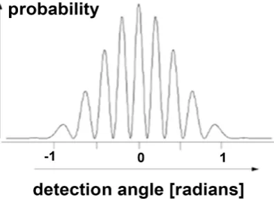
.DOI: 10.4236/jmp.2019.104027 430 Journal of Modern Physics profile by the two-slit interference. In Figure 6 we show an example using B/λDB
= 5 to calculate the two slit modulation, and d = λDB to calculate the diffraction
profile. At this width we have d = Δx = λDB, and a width of the diffraction peak
corresponding to Δp = p = ħ/λDB, so that the uncertainty relation inherent in the
model becomes ΔpΔx = ħ.
As the main result of the present paper we state that the two-slit quantum in-terference is correctly described without quantum mechanics.
3. Conclusion and Discussion
The dynamic substructure, which the model ascribes to the particle, explains the two slit interference, one of the main quantum phenomena, without using quantum mechanics. In a similar way, energy quantization of bound states, as well as angular momentum quantization, is predicted by the model in agreement with observation. In addition, as has been shown in the previous papers [10] [11], the properties of the electron, mass, spin, and magnetic moment, follow from the substructure implied by the model. Further, the paradox of “wave-particle dualism” does not arise, because “wave interference” is explained as “particle in-terference”.
As already mentioned, the model is based on the idea that spin might be ex-plained as angular momentum caused by a quantum of momentum (mc) when it passes a fixed point in space. The completed model of an elementary particle, used in this paper, may be visualized in a very simple way: The point (Ph) (see
Figure 1), which is located in the center of the circle containing the quantum, is identified as a photon, and the point, which is located in the center of this circu-lating photon, is identified as the particle. As shown in Figure 4, the photon forms a spiraling trace with tangential speed (c), independent of the relative mo-tion (v) with respect to an observer, and its energy is pc = mc2, with
(
)
(
2)
0 1
m=m √ −β . The momentum component of the photon in direction of
[image:8.595.279.479.526.670.2]relative motion,
(
mv
=
m c
β
=
m c n
0)
, is the momentum of the “particle”.DOI: 10.4236/jmp.2019.104027 431 Journal of Modern Physics There remain important questions regarding the validity of the model. On the other hand, in our opinion, its demonstrated successes are too manifold and substantial to be accidental. Therefore, a thorough theoretical investigation of the model, especially of its relation to quantum field theory, seems interesting.
Conflicts of Interest
The author declares no conflicts of interest regarding the publication of this pa-per.
References
[1] Messiah, A. (1964) Quantum Mechanics. Vol. II, North Holland Publishing Com-pany, Amsterdam, 540.
[2] Khrennikov, A. (2017) Foundations of Physics, 47, 1077-1099. https://doi.org/10.1007/s10701-017-0089-0
[3] Schroedinger, E. (1930) Sitzungsber. Preuss. Akad. Wiss. Phys.-Math. Kl.,24, 418. [4] Hestenes, D. (1979) American Journal of Physics, 47, 399-415.
https://doi.org/10.1119/1.11806
[5] Hestenes, D. (1990) Foundations of Physics, 20, 1213-1232. https://doi.org/10.1007/BF01889466
[6] Hestenes, D. (2003) Annales de la Fondation Louis de Broglie,28, 390-408. [7] Barut, A.O. and Sanghi, N. (1984) Physical Review Letters,52, 2009-2012.
https://doi.org/10.1103/PhysRevLett.52.2009 [8] Vaz Jr., J. (1995) Physics Letters B, 344, 149-157.
https://doi.org/10.1016/0370-2693(94)01548-Q
[9] Pavsic, M., Recami, E., Waldyr, A., Rodriges Jr., G., Maccarrone, D., Racciti, F. and Salesi, G. (1993) Physics Letters B, 318, 481-488.
https://doi.org/10.1016/0370-2693(93)91543-V [10] Niehaus, A. (2016) Foundations of Physics,46, 3-13.
https://doi.org/10.1007/s10701-015-9953-y
[11] Niehaus, A. (2017) Journal of Modern Physics, 8, 511-521. https://doi.org/10.4236/jmp.2017.84033