Short and Long Term Time Series Forecasting Stochastic Analysis for Slow Dynamic Processes

(1)

ISSN Online: 2152-7393 ISSN Print: 2152-7385

DOI: 10.4236/am.2019.108050 Aug. 27, 2019 704 Applied Mathematics

Short and Long-Term Time Series Forecasting

Stochastic Analysis for Slow Dynamic Processes

Julián Pucheta

1

_{, Carlos Salas}

2

_{, Martín Herrera}

2

_{, Cristian Rodriguez Rivero}

3

_{, Gustavo Alasino}

4

1_{FCEFyN-Universidad Nacional de Córdoba, Córdoba, Argentina}

2_{FTyCA-Universidad Nacional de Catamarca, Catamarca, Argentina}

3_{Cristian University of California, Los Angeles, USA}

4_{Universidad Torcuato Di Tella, Buenos Aires, Argentina}

Abstract

This paper intends to develop suitable methods to provide likely scenarios in order to support decision making for slow dynamic processes such as the un-derlying of agribusiness. A new method to analyze the short- and long-term time series forecast and to model the behavior of the underlying process using nonlinear artificial neural networks (ANN) is presented. The algorithm can effectively forecast the time-series data by stochastic analysis (Monte Carlo) of its future behavior using fractional Gaussian noise (fGn). The algorithm was used to forecast country risk time series for several countries, both for short term that is 30 days ahead and long term 350 days ahead scenarios.

Keywords

Stochastic Analysis, Time Series Forecasting, Decision Making, Dynamic Process, Process Modelling

1. Introduction

The agribusiness activities are the engine where the vegetal production lies with its decision-making built-in [1]. In Argentina, the activity’s profit is subjected to a good production plan which in turn is subjected to financial variables [2]. One of them is the Emerging Market Bond Index (EMBI) known as country risk. This variable indexes the economic health of the country and is a strong signal when is compared against that of Chile, Brazil and Mexico countries whose products compete with those of Argentinian. When the producer must perform the production plan, there arises the need for counting with information about the EMBI values with some future horizon. In this paper, a method to forecast time series from EMBI with short and long term horizons is proposed.

How to cite this paper: Pucheta, J., Salas, C., Herrera, M., Rodriguez Rivero, C. and Alasino, G. (2019) Short and Long-Term Time Series Forecasting Stochastic Analysis

for Slow Dynamic Processes. Applied

Ma-thematics, 10, 704-717.

https://doi.org/10.4236/am.2019.108050

Received: July 25, 2019 Accepted: August 24, 2019 Published: August 27, 2019

(2)

DOI: 10.4236/am.2019.108050 705 Applied Mathematics

The article is structured as follows: after this Introduction, Section 2 describes an overview of the problem statement. Section 3 shows the proposed approach of the training and the selection method based on fractional Brownian motion using classical non-linear autoregressive model based on neural networks. Sec-tion 4 shows the sets of monthly EMBI series from Latin America countries, with emphasis on the statistical evaluation of the short-range case (800 training data samples) and the long-range (2700 training data). Section 5 presents some dis-cussions and concluding remarks.

2. Problem Formulation

When agricultural venture is focused on profit from production purposes, sever-al dynamic rates arises. One of them, the very short-term dynamic embraces process such as irrigations and nutrients, chemical applications in which it must take that decision [3]. Another dynamic arises when the producer plans the crop to sow and the rainfall forecast is required to perform such a task at an optimal date decision [4] [5] [6] [7]. However, the slow dynamic process related with the final product offer and demand is the variable with special interest in the agro-nomic venture which is subject to future ecoagro-nomic scenario [8].

Is in this scenario where earn importance some economic variables, specifi-cally the EMBI [9] whose role serves to measure the economic health of a coun-try. So, in order to take optimal decision in the choice of crop and date, the availa-bility of some economic future information about some player is required. There-fore, future scenarios from economic health in Argentina, Chile and Brazil in short and long term gives information to improve such decision making [10].

3. Proposed Approach

In this paper, a classical non-linear autoregressive model based on neural net-works whose parameters are batch tuned [11] and its performance is evaluated by stochastic analysis is proposed [12].

After training is completed, predictions are generated by using Monte Carlo with Gaussian noise (Gn) and fGn [13]. The expectation from each prediction ensemble is computed for obtaining a deterministic time series both for Gn and fGn. The stochastic analysis of these time series is performed for determining the forecast with the appropriate stochastic roughness characteristic and so it is chosen for the forecast. This section details the training and the selection me-thod based on fGn.

3.1. The Basic Problem

The classical prediction problem can be formulated as follows. Given past values

uniformly time-spaced of a process, namely x n

(

−1 ,

) (

x n−2 , ,

)

 x n N

(

−

)

where

N is the time series length, the present value x(n) must be predicted.

Here, a prediction device is designed by considering the given sequence {xn} at

(3)

for the following future 30/350 values sequence. Hence, it is proposed a predic-tor filter with an input vecpredic-tor x, which is obtained by applying the delay operapredic-tor

D, to the sequence {xn}. Then, the filter output will generate xe as the next value,

that will be best estimate of the present value xn. So, the prediction error at time

k can be evaluated as

( )

n

( )

e

( )

e k =x k −x k (1)

which is used for the learning rule to adjust the NN weights.

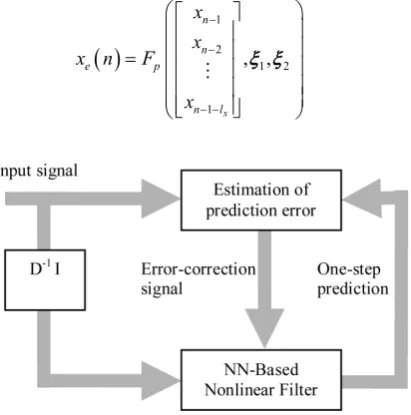
The predictor is implemented by an autoregressive neural network-based non-linear adaptive filter. The NNs are used as a nonnon-linear model building to represent the underlying physical process dynamic behavior that generates the data. In this work, time lagged feed-forward networks are used.

The present value of the time series is used as the desired response for the adaptive filter, and the past values of the signal are supplied as adaptive filter in-put. Then, the adaptive filter output will be the one-step prediction signal. In Fig-ure 1 the block diagram of the nonlinear prediction scheme based on a NN filter is shown. Therefore, our aim is to obtain the best prediction (in roughness sense) of the present values from a random (pseudo-random) time series.

3.2. NN-Based AR Model

Several experiences had been obtained from previous works detailed in [12]. Here, an NN-based AR filter model is tuned. The NN used is a time lagged feed-forward

networks class. The NN topology consists of lx inputs, one hidden layer of Ho

neurons that are the processing nodes in the hidden layer, and one output neu-ron as shown [12]. The learning rule used in the learning process is based on the Levenberg-Marquardt method [14].

In order to predict the sequence {xe} one-step ahead, the first delay is taken

from the tapped-line xn and used as input. Therefore, the output prediction can

be denoted by

( )

1

2

1 2

1

, ,

x

n

e p

n l

x x

x n F

x

− −

  

  

= __ _ _

  

__ __ 

 

[image:3.595.273.479.500.708.2]

 ξ ξ (2)

(4)

where, Fp

(

⋅, ,ξ ξ1 2

)

is the nonlinear predictor filter with lx inputs and xe(n) is

the output prediction at time n. In addition, ξ1 and ξ2 contain the tuning

pa-rameter composed by

1 2

1=  1 1  1Ho

ξ ξ ξ ξ ₍₃₎

whose elements are arrays defined as

1 1i∈ℜlx+

ξ (4)

and

1 2∈ℜHo+

ξ (5)

where Ho is the number of processing nodes. Thus, the predictor filter contains

tuning parameters ξ1 and ξ2 that must be computed and from now on will

not be explicit to avoid notation abuse.

3.3. Monte Carlo Implementation Including Fractional Brownian

Motion

In this work the Hurst’s parameter is used as statistical criteria for time series forecast by selecting the assessment in the algorithm. This H gives an idea of signal roughness, and determines its stochastic dependence, here is implemented according to [15]. The definition of the Hurst’s parameter appears in the Brow-nian motion from generalizing the integral to a fractional one. The Fractional Brownian motion (fBm) is defined in the pioneering work by Mandelbrot [16] [17] through its stochastic representation

( )

0

(

)

1

( )

1

( )

(

)

1

( )

2 2 2

0

1 _d _d

1 2

t

H H H

H

B t t s s B s t s B s

H

− − −

−∞

   

= _ _ − − − _ + − _

    

Γ_ + _

 

∫

(6)

where, Γ_{(·) represents the Gamma function}

( )

1

0 e d

x

xα x

α ∞ − −

Γ =

_∫

(7)

and 0<H<1_{is called the Hurst parameter. The integrator B is a stochastic}

process, ordinary Brownian motion. The determination of H results in a

sto-chastic process with more roughness (H < 1/2) or more smoothness (H > 1/2)

which is fixed given the real processes evidences. Note, that B is recovered by taking H = 1/2 in (6). Here, it is assumed that B is defined on some probability space (Ω, F, P), where Ω, F and P are the sample space, the sigma algebra (event space) and the probability measure respectively. Thus, an fBm is a time

conti-nuous Gaussian process depending on the so-called Hurst parameter 0<H<1_.

The ordinary Brownian motion is generalized to H = 0.5, and whose derivative is the white noise. The fBm is self-similar in distribution and the variance of the increments is defined by

( )

(

)

2H

H H

Var B t −B s = ⋅ −

ν

t s ₍₈₎

(5)

This special form of the variance of the increments suggests various ways to estimate the parameter H. In fact, there are different methods for computing the

parameter H associated to Brownian motion [17]. In this work, the algorithm

uses a wavelet-based method for estimating H from a trace path of the fBm with parameter H [18]. To generate data, as example, three ensemble from fBm with different values of H are shown in Figure 2, where can be noted the difference in the variances for each H. The figure shows synthetized traces using the method described in [13], where the black dots corresponds to five traces for each H, the magenta lines shows the theoretical variances using (8) and the blue lines shows the variance estimated by

( )

(

[ ]

)

2

,

1

t t t

Var f f E f

N ω ω

=

∑

− ₍₉₎

where N is the size of f(t, ω) for each time t. and ω indicates each trace. Finally, in this paper the method implemented in [15] was used.

3.4. Algorithm Description

[image:5.595.213.533.427.680.2]

Our thesis asserts that if some process evolves along time with any H, it will do in the future with the same H namely keeping its smoothness or roughness. To do so, a classic non-linear model based on neural networks batch-tuned is pro-posed. In the tuning process, data are randomly split for generalizing and train-ing, with a 15% and 85% ratio, respectively. Furthermore, since the last data are the most important given the series nature, the last or the last two are left for

(6)

evidence test. Thus, the relevant data quantity to be considered from the series is them determined for performing the desired forecast. By this way the parameters for Equation (3) are obtained.

After tune the filter defined in Equation (2), the predictions are generated us-ing normal Gaussian and fractional Gaussian noise. In order to generate the en-semble with R traces for forecasting the time series, it is modified the Equation (2) by

(

)

(

)

1

2

1

, , ,

x

n q

e p H

n q l

x x

x n q F B q

x

ω ω θ ω

− + − +

− + −

  

  

+ = __ _ _+ ⋅ ∆

  

__ __ 

 

 (10)

where q=1,2, , FH sets the future time, FH the forecast horizon, ω=1,2, , R

denotes each trace, R is the ensemble size and θ is a parameter for denormalizing

BH. For selecting a fixed value for θ, one must take into account the length of the

forecast horizon FH, which in this work are 30 and 350 days and also the series

dynamic range, using

( )

_{( )}

( )

2

max min

1

max

H

x x

F x

θ₌ _ − _

 

 _ _

 

(11) and specifically when H = 0.5 the Gaussian case is obtained. The coefficient θ was introduced for normalizing the ensemble along the forecast time. The en-semble described by Equation (10) is analyzed by classical statistical methods for obtaining the mean and the variance functions.

Once the tuning process is completed, for the short term forecast case a se-quences pair is defined. One sequence is

{ }

xn , n=1,2,3, , N (12)

and the other is composed by the former concatenated with the forecasted which is the ensemble expectation from Equation (10), that is

{ }

{

[ ]

}

{

xn , E xe

}

, 1,2,3, ,e=  FH (13)

Both sequences are analyzed by the method detailed in [18] and such esti-mated H must match between (12) and (13). Thus, ensemble mean of each pre-diction is taken and that one with the suitable stochastic roughness H is chosen as the forecast. Table 1 details the method for tuning and selecting based on fBm.

4. Implementation with EMBI Time Series

The method has been implemented by considering that there are more than 2700 data values from several countries.

(7)

DOI: 10.4236/am.2019.108050 710 Applied Mathematics Table 1. Algorithm that performs the short/long term time series forecast.

1. Set the neural network (NN) topology by assigning lx, Ho Equation (4) Equation (5).

2. Chose the data for truth test that are just one or two of the last time series data that will not be _{used by training or validating processes.}

3. Train the NN with 85% of the data and check the overfitting with the remaining 15%. 4. Stop the training if the generalization error increases.

5. If the truth test data is not suitably forecasted, go to 1. 6. Set H = 0.5, set θ via Equation (11).

7. Run Monte Carlo including H described by Equation (10).

8. Select the mean value that gives the best match of H according to the long or the short range _scenario.

9. The obtained mean series generated and its variance are the algorithm results.

10. Given the case that the results were not credible, go to 6 and modify the noise characteristic by _{changing H, 0 < H < 1.}

the methodology uses a batch training with a validation set of 15% of the ran-dom data set. In the short-range case, 800 training values were used and for the long-range, 2700.

The last group of one to three data was left as a test of disruptive validation or truth test, mainly for studying the overfitting. The prediction was made by Monte Carlo simulation where the noise used were stationary, seasonal and pseudoran-dom, although with a roughness characteristic determined by the Hurst para-meter, generated by using [15].

The roughness is evaluated by the Hurst’s parameter H, which is computed using a wavelet-based method [18]. After the tuning process is completed, two sequences pairs are defined. One pair is

{ }

xn , n=1,2,3, , NS (14)

with

{ } { }

{

xn , xe

}

, 1,2,3, ,e=  FS (15)

for the short term forecast given NS =800, FS =30. The other pair is

{ }, 2350,2351, ,

xn n=  NL (16)

with

{ } { }

{

xn , xe

}

, 1,2,3, ,e=  FL (17)

for the long term forecast given NL =2700, FS =350. The selection of NL was

determined given the available data samples, and the parameter FS was

deter-mined given that one year ahead is long term for development countries. Each pair of sequences must show the same H parameter estimated by [18].

4.1. Monthly EMBI Forecast

(8)

30 step ahead. The time series belong to EMBI from Argentina, Chile, Brazil and Mexico. The results are summarized in Table 2, and the evolution over time is shown in Figures 3-6. The images shown a shaded area that indicates the ensem-ble range, 100% of the traces, obtained by Monte Carlo. Inside the shaded area is

Table 2. Roughness results with the implementation of the 30-day algorithm (March 2019).

Series Argentina Chile Brazil Mexico

{xn} 0.66917 0.503 0.63827 0.65115

{xn, xe} fGn 0.66941 0.49902 0.63864 0.65077

Figure 3(a) Figure 4(a) Figure 5(a) Figure 6(a)

{xn,xe} Gn 0.66895 0.50227 0.6376 0.65128

Figure 3(b) Figure 4(b) Figure 5(b) Figure 6(b)

Figure 3. Argentinean EMBI forecast and its stochastic roughness up to Jan 2019. The cyan line is the data samples, the yellow area depicts the 100% of the Monte Carlo traces, the orange area indicates the 66% of the traces, and the red line is the mean value of the stochastic process.

(a) H = 0.66941; (b) H = 0.66895.

Figure 4. Chilean EMBI forecast and its stochastic roughness up to Jan 2019. (a) H = 0.49902;

(b) H = 0.50227.

0 2 4 6 8 10 12 14

26-Nov-2018 06-Dec-2018 16-Dec-2018 26-Dec-2018 05-Jan-2019 15-Jan-2019 25-Jan-2019

0 5 10 15

(a) (b)

0 0.5 1 1.5 2 2.5 3 3.5

(9)

[image:9.595.162.538.60.253.2]

DOI: 10.4236/am.2019.108050 712 Applied Mathematics Figure 5. Brazilian EMBI forecast and its stochastic roughness up to Jan 2019. (a) H = 0.63864; (b) H = 0.6376.

Figure 6. Mexican EMBI forecast and its stochastic roughness up to Jan 2019. (a) H = 0.65077; (b) H = 0.65128.

another shaded area that indicates the 66% of the traces. The statistic indicator is H, which is detailed under each ensemble. The aim of show values of H, cases (a) and (b) of each series, is to highlight the behavior of the forecast. The case of the ensemble generation with H = 0.5 is shown in the lower rows of the table, given that the estimation of H gives figures near 0.5. In Table 2 are summarized the results, where the values in bold fonts indicates the forecast recommended by the criteria stated in this work.

4.2. Annual EMBI Forecast

The algorithm of Table 1 is used for forecasting long term periods, in this case 350 steps ahead. The simulation conditions are those of Equation (16) and Equa-tion (17). Here, the Monte Carlo was set with fracEqua-tional Gaussian noise and normal Gaussian noise, detailed in different rows of Table 3. The figures in bold

(a) (b) 0

0.5 1 1.5 2 2.5 3 3.5 4 4.5 5

0 1 2 3 4 5 6

(a) (b) -2

-1 0 1 2 3 4 5

-4 -3 -2 -1 0 1 2 3 4 5

[image:9.595.159.538.299.483.2]

(10)

DOI: 10.4236/am.2019.108050 713 Applied Mathematics Table 3. Roughness results with the implementation of the algorithm for 350 days hori-zon forecast (Dec 2019).

Series Argentina Chile Brazil Mexico

{xn} 0.70392 0.40106 0.647 0.54395

{xn,xe} fGn 0.78425 0.6938 0.6444 0.29233

Figure 7(a) Figure 8(a) Figure 9(a) Figure 10(a)

{xn,xe} Gn 0.58782 0.47213 0.44172 0.83236

Figure 7(b) Figure 8(b) Figure 9(b) Figure 10(b)

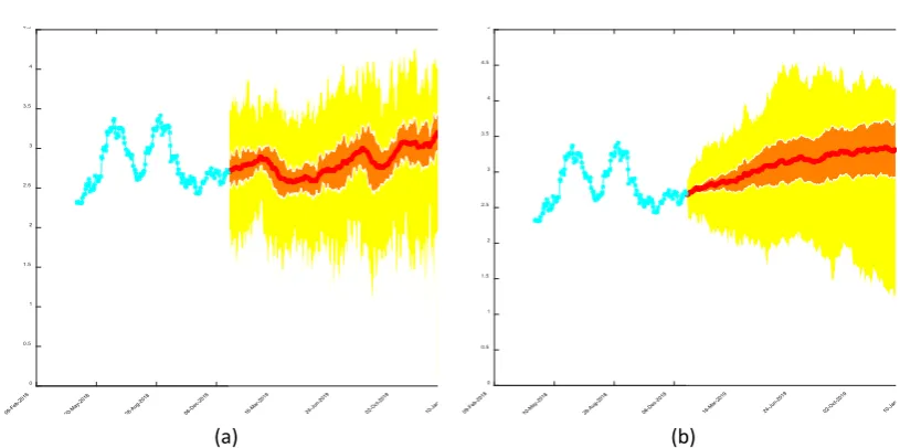
Figure 7. Argentinean EMBI forecast and its stochastic roughness up to Dec 2019. The cyan line is the data samples, the yellow area depicts the 100% of the Monte Carlo traces, the orange area indicates the 66% of the traces, and the red line is

the mean value of the stochastic process. (a) H = 0.78425; (b) H = 0.58782.

Figure 8. Chilean EMBI forecast and its stochastic roughness up to Dec 2019. (a) H = 0.6938; (b) H = 0.47213.

(a) (b)

0

2 4 6 8 10 12

09-Feb-2018 20-May-2018 28-Aug-2018 06-Dec-2018 16-Mar-2019 24-Jun-2019 02-Oct-2019 10-Jan-2020

0 5 10 5

(a) (b)

0

0.5 1 1.5 2 5

0 0.5 1 1.5 2 2.5 3

(11)

[image:11.595.130.538.62.265.2]

DOI: 10.4236/am.2019.108050 714 Applied Mathematics Figure 9. Brazilian EMBI forecast and its stochastic roughness up to Dec 2019. (a) H = 0.6444; (b) H = 0.44172.

Figure 10. Mexican EMBI forecast and its stochastic roughness. (a) H = 0.29233; (b) H = 0.83236.

show the preferred forecast of this method. The shaded areas embrace the traces from the ensemble, where the darkest indicates the 66% of confidence and the continuous thick line is the mean value.

4.3. Discussion

From our results, the obtained EMBI behavior is stable with increasing trend in the Argentina’s case, which is very volatile. The EMBI behavior shows a decreasing trend in the Mexico’s case. The variation ranges estimated for Argentina is very broad although by tuning the H parameter it can be narrowed. At the regional level, the variations of Chile and Brazil forecasted EMBI are moderate and the one of Mexico are very small.

The trend indicates a fall in the quarter and then continues declining respect of the range the historical. Volatility affects the amplitude of the range with

pre-(a) (b) 0

0.5 1 1.5 2 2.5 3 3.5 4 4.5

0 0.5 1 1.5 2 2.5 3 3.5 4 4.5 5

(a) (b) 0

1 2 3 4 5 6

0 0.5 1 1.5 2 2.5 3 3.5 4 4.5 5

[image:11.595.130.537.302.493.2]

(12)

dicted values with probable values of descent around 495 basis points (bp) in less than 90 days.

The scenario of variations is high, but with a decreasing trend with wide mar-gins conditioned by the high fluctuation of its historical index behavior. The av-erage monthly value is around 700 bp and with an annual downward trend. This is an acceptable forecast given that 2019 is a year with scheduled presidential elections in Argentina.

For Chile’s case, the study starts around 165 bp with an upward, soft and con-stant trend that continues up to the end of March with 160 points, which indi-cates some internal or external factor that slightly presses the upside. For its part, according to this model Brazil will start the year around 272 bp and it would have an ascending behavior no higher than 290 until March 20 when it starts to return to 260, with small variation and regular movements without brusque highs and lows. Finally, in the case of Mexico, the prediction that it would begin in the range 350 - 360 bp, with a smooth descending trend towards the end of January 330 - 300 bp, and the rest of the quarter remains in 325 - 350 is also ac-ceptable.

It can be concluded that the likely economic scenarios for agribusiness pro-ducers is competitive but very similar to that of prior years, so taking care this highlights the final product will be well positioned.

5. Conclusions

In this work, a methodology based on neural networks filter to model the un-derlying process behavior that causes the EMBI measurements evolution of the short and long term was detailed. The methodology consists of generating an ar-tificial intelligence based predictor filter with a stochastic analysis of its future behavior using fractional Gaussian noise. Results of this analysis were shown to determine which series is the most coincident according to the Hurst parameter.

The generated information is not the exact value, but gives an idea about which will be the index trend based on its historical values intended for slow dynamic processes. The incorporation of this variable into decision making by estimating the predicted values impacts on the business plan or the investment portfolio. In the latter case, the EMBI provides a daily measure of the investor’s perception regarding country risk. Thus, given the alarm sense that brings the EMBI rise, it is relevant to generate the projection of this series for the region and some countries that comprise it. Based on data predictions, it is possible to optimize the expo-sure in instruments, both bonds as shares, at country level and help to reduce the exposure in moments that anticipate an EMBI increase.

(13)

sce-DOI: 10.4236/am.2019.108050 716 Applied Mathematics

nario of the required return rate in dollars of the countries under analysis and allows the portfolio manager to reaffirm investment and exposure objectives considering the individuality of the risk of each country and the whole, or re-formulate the investment.

Conflicts of Interest

The authors declare no conflicts of interest regarding the publication of this pa-per.

References

[1] Car, N.J. (2018) USING Decision Models to Enable Better Irrigation Decision

Sup-port Systems. Computers and Electronics in Agriculture, 152, 290-301.

https://doi.org/10.1016/j.compag.2018.07.024

[2] Rupnik, R., Kukar, M., Vračar, P., Košir, D., Pevec, D. and Bosnić, Z. (2018)

AgroDSS: A Decision Support System for Agriculture and Farming. Computers and

Electronics in Agriculture, 161, 260-271.

[3] Prabakaran, G., Vaithiyanathan, D. and Ganesan, M. (2018) Fuzzy Decision

Sup-port System for Improving the Crop Productivity and Efficient Use of Fertilizers.

Computers and Electronics in Agriculture, 150, 88-97.

[4] Alugubelly, M., Polepalli, K.R., Gade, S. and Ninomiya, S. (2019) Analysis of Similar

Weather Conditions to Improve Reuse in Weather-Based Decision Support

Sys-tems. Computers and Electronics in Agriculture, 157, 154-165.

[5] Li, Z.H., He, J.Q., Xu, X.G., Jin, X.L., Huang, W.J., Clark, B., Yang, G.J. and Li, Z.H.

(2018) Estimating Genetic Parameters of DSSAT-CERES Model with the GLUE

Method for Winter Wheat (Triticum aestivum L.) Production. Computers and

Electronics in Agriculture, 154, 213-221.

[6] Rivero, C.R., Pucheta, J., Sauchelli, V. and Patiño, H.D. (2016) Short Time Series

Prediction: Bayesian Enhanced Modified Approach with Application to Cumulative

Rainfall Series. International Journal of Innovative Computing and Applications, 7,

153-162.https://doi.org/10.1504/IJICA.2016.078730

[7] Rivero, C.R., Patiño, D., Pucheta, J. and Sauchelli, V. (2016) A New Approach for

Time Series Forecasting: Bayesian Enhanced by Fractional Brownian Motion with

Application to Rainfall Series. International Journal of Advanced Computer Science

and Applications, 7, 237-244. https://doi.org/10.14569/IJACSA.2016.070334

http://thesai.org/Publications/ViewPaper?Volume=7&Issue=3&Code=ijacsa&Serial No=34#sthash.ETZInPQR.dpuf

[8] Cavanagh, J. and Long, R. (1999) Introducing the J.P. Morgan Emerging Markets

Bond Index Global (EMBI Global). J.P. Morgan Securities Inc. Emerging Markets Research, New York.

https://faculty.darden.virginia.edu/liw/emf/embi.pdf [9] https://www.imf.org/external/pubs/ft/wp/2015/wp15263.pdf

[10] https://www.invenomica.com.ar/riesgo-pais-embi-america-latina-serie-historica

(14)

Network. Twenty-Third Annual Hawaii International Conference on System

Sciences, Kailua Kona, 2-5 January 1990, 327-334.

[12] Rivero, C.R., Pucheta, J., Laboret, S. and Sauchelli, V. (2017) Energy Associated

Tuning Method for Short-Term Series Forecasting by Complete and Incomplete

Datasets. Journal of Artificial Intelligence and Soft Computing Research, 7, 5-16.

https://doi.org/10.1515/jaiscr-2017-0001

[13] Hosking, J.R.M. (1984) Modeling Persistence in Hydrological Time Series Using

Fractional Brownian Differencing. Water Resources Research, 20, 1898-1908.

https://doi.org/10.1029/WR020i012p01898

https://agupubs.onlinelibrary.wiley.com/doi/epdf/10.1029/WR020i012p01898

[14] Marquardt, D. (1963) An Algorithm for Least-Squares Estimation of Nonlinear

Pa-rameters. SIAM Journal on Applied Mathematics, 11, 431-441.

https://doi.org/10.1137/0111030

[15] http://www.columbia.edu/~ad3217/fbm/hosking.c

[16] Mandelbrot, B.B. and Van Ness, J.W. (1968) Fractional Brownian Motions,

Frac-tional Noises and Applications. SIAM Review, 10, 422-437.

https://doi.org/10.1137/1010093

[17] Dieker, T. (2004) Simulation of Fractional Brownian Motion. MSc Theses,

Univer-sity of Twente, Amsterdam.

[18] Abry, P., Flandrin, P., Taqqu, M.S. and Veitch, D. (2003) Self-Similarity and

Long-Range Dependence through the Wavelet Lens. In: Doukhan, P., Oppenheim,

G. and Taqqu, M., Eds., Theory and Applications of Long-Range Dependence,