Multivariate selection and intersexual genetic constraints in a wild bird population
1
Jocelyn Poissant1,2, Michael B. Morrissey3, Andrew G. Gosler4, Jon Slate2, Ben C. Sheldon4
2
3
1Centre for Ecology and Conservation, College of Life and Environmental Sciences, University
4
of Exeter, Penryn, UK
5
2Department of Animal and Plant Sciences, University of Sheffield, Sheffield, UK
6
3School of Biology, University of St Andrews, St Andrews, UK
7
4Edward Grey Institute, Department of Zoology, University of Oxford, Oxford, UK
8
9
Running title: Multivariate intralocus sexual conflict
10
Correspondence
11
Jocelyn Poissant
12
Centre for Ecology and Conservation, College of Life and Environmental Sciences, University of
13
Exeter, Penryn, Cornwall, TR10 9FE, UK. Telephone: +44 (0)1326 370400; Fax: +44 (0)1326
14
371859; e-mail: [email protected]
15
16
17
18
19
20
21
22
23
24
25
Abstract
27
When selection differs between the sexes for traits that are genetically correlated between the
28
sexes, there is potential for the effect of selection in one sex to be altered by indirect selection in
29
the other sex, a situation commonly referred to as intralocus sexual conflict (ISC). While
30
potentially common, ISC has rarely been studied in wild populations. Here, we studied ISC over
31
a set of morphological traits (wing length, tarsus length, bill depth, and bill length) in a wild
32
population of great tits (Parus major) from Wytham Woods, UK. Specifically, we quantified the
33
microevolutionary impacts of ISC by combining intra- and inter-sex additive genetic
34
(co)variances and sex-specific selection estimates in a multivariate framework. Large genetic
35
correlations between homologous male and female traits combined with evidence for
sex-36
specific multivariate survival selection suggested that ISC could play an appreciable role in the
37
evolution of this population. Together, multivariate sex-specific selection and additive genetic
38
(co)variance for the traits considered accounted for additive genetic variance in fitness was
39
uncorrelated between the sexes (cross-sex genetic correlation = -0.003, 95% CI = -0.83, 0.83).
40
Gender load, defined as the reduction in a population’s rate of adaptation due to sex-specific
41
effects, was estimated at 50% (95% CI = 13%, 86%). This study provides novel insights into the
42
evolution of sexual dimorphism in wild populations and illustrates how quantitative genetics and
43
selection analyses can be combined in a multivariate framework to quantify the
44
microevolutionary impacts of ISC.
45
46
Keywords: G matrix, genetic correlation, intralocus sexual conflict, selection gradient, sexual
47
dimorphism, animal model, heritability, natural selection, quantitative genetics, gender load
48
49
50
51
Introduction
53
Males and females in dioecious species are typically dimorphic for a large number of phenotypic
54
traits (Fairbairn et al., 2007). Such sexual dimorphism is generally believed to be adaptive,
55
reflecting difference in sex-specific phenotypic optima (Fairbairn, 2007). While the widespread
56
occurrence of sexual dimorphism indicates that its evolution is possible, large genetic
57
correlations between most homologous male and female traits suggest that its short-term
58
evolution may be constrained (Lande, 1980; Poissant et al., 2010). Indeed, whenever selection
59
differs between the sexes for traits that are genetically correlated between the sexes, there is
60
potential for the effect of selection in one sex to be altered by indirect selection in the other sex,
61
a situation generally referred to as intralocus sexual conflict (ISC) or gender load (Arnqvist &
62
Rowe, 2005; Bedhomme & Chippindale, 2007; Bonduriansky & Chenoweth, 2009; Pennell &
63
Morrow, 2013). While potentially common and important, such intersexual genetic constraints
64
remain little studied in wild populations (Bonduriansky & Chenoweth, 2009; Pennell & Morrow,
65
2013; Poissant et al., 2010; Wyman et al., 2013).
66
67
The evolutionary forces acting on sexual dimorphism depend on the interaction between
sex-68
specific genetic (co)variances and directional selection, as represented by the Lande (1980)
69
sex-specific version of the Lande (1979) equation:
70
71
72
Δ𝑧! Δ𝑧! =
!
!
𝐆! 𝐁
𝐁! 𝐆
!
!!
!! (1)
73
74
75
where Δ𝑧! andΔ𝑧! are vectors of male and female specific responses, Gm and Gf are
sex-76
specific additive genetic covariance matrices, B and BT are matrices of cross-sex additive
genetic covariances, and 𝛽! and 𝛽! are sex-specific vectors of selection gradients. The
78
coefficient of one half is included to account for the fact that selected male and female parents
79
make equal autosomal contributions to offspring of both sexes (Lande, 1980). Despite being
80
well known among evolutionary biologists studying sexual dimorphism, surprisingly few have
81
applied the Lande (1980) equation in wild populations (though see Jensen et al., 2008, Stearns
82
et al., 2012, Tarka et al., 2014, and Walling et al., 2014, for rare examples). Instead, studies
83
typically focus on estimating either only sex-specific selection (Cox & Calsbeek, 2009) or
84
quantitative genetic parameters (Poissant et al., 2010). In addition, while equation 1 is explicitly
85
multivariate, most quantitative genetic studies of sexual dimorphism performed to date have
86
focused on univariate traits (Wyman et al., 2013). As a consequence, we still know relatively
87
little about the structure of the B matrix and its impact on the evolution of sexual dimorphism
88
(Gosden et al., 2012; Wyman et al., 2013). For example, asymmetry of the B matrix (differences
89
between below- and above-diagonal elements) may play an important role in facilitating the
90
evolution of multivariate sexual dimorphism (Wyman et al., 2013), but too few B matrices have
91
been published to assess the importance of this mechanism (Barker et al., 2010; Wyman et al.,
92
2013). Studies combining sex-specific selection and quantitative genetic parameters, and
93
especially those doing so in a multivariate framework, are therefore needed (Walsh & Blows,
94
2009; Wyman et al., 2013).
95
96
Genetic constraints on the evolution of sexual dimorphism may be widespread (Bonduriansky &
97
Chenoweth, 2009; Cox & Calsbeek, 2009; Pennell & Morrow, 2013; Poissant et al., 2010). In
98
particular, negative cross-sex genetic correlations (rmf) for lifetime fitness in wild populations
99
have been reported (e.g. Brommer et al., 2007; Foerster et al., 2007), and rmf for fitness
100
components are on average lower than for other trait categories (Poissant et al., 2010).
101
However, little is known about the traits underlying these cross-sex genetic correlations for
102
fitness and their relative importance (Bonduriansky & Chenoweth, 2009; Pennell & Morrow,
2013). In part, this is because research tends to be qualitative rather than quantitative, with
104
publications focusing on the statistical significance of intralocus sexual conflicts rather than
105
quantifying their impacts on microevolution.
106
107
A variety of metrics have been developed to quantify multivariate genetic constraints (Walsh &
108
Blows, 2009), and researchers have started applying them to studies of sexual dimorphism in
109
both laboratory (Gosden et al., 2012; Lewis et al., 2011) and wild (Stearns et al., 2012; Tarka et
110
al., 2014; Walling et al., 2014) populations. However, in many cases, differences in data
111
transformation and standardization make comparison of results across traits and studies difficult
112
(Hansen & Houle, 2008; Houle et al., 2011). In addition, not all metrics provide easily
113
interpretable or comparable quantitative information (Hansen & Houle, 2008). One approach
114
that is particularly valuable for the study of ISC is the R metric of Agrawal and Stinchcombe
115
(2009). This metric quantifies the impact of genetic covariances on a population’s rate of
116
adaptation, including the specific case of cross-sex genetic covariances. Importantly, it yields
117
results that are readily comparable across sets of traits, populations and species (Agrawal &
118
Stinchcombe, 2009). Despite its potential for improving our understanding of ISC, to date few
119
have applied the approach in that context (see Walling et al., 2014, for a rare example).
120
121
The importance of considering multivariate phenotypes in studies of ISC is increasingly being
122
recognized (Wyman et al., 2013). However, conducting multivariate quantitative genetic studies
123
in wild populations remains challenging, due to difficulties in acquiring sufficiently large
124
pedigree-linked datasets (Wilson & Poissant, 2016). In this study, we take advantage of a
long-125
term study of individual variation in morphological traits (wing length, tarsus length, bill depth
126
and bill length) conducted over multiple decades in a wild pedigreed population of great tits
127
(Parus major) from Wytham Woods, Oxford, UK (Savill et al., 2010), to quantify the
128
microevolutionary impacts of ISC in a wild population. Despite being a model organism for
evolutionary ecology research, surprisingly little is currently known about the genetic basis of
130
homologous male and female traits and ISC in this species. This could be due to the fact that
131
morphological traits routinely measured in field studies such as wing and tarsus length are not
132
particularly sexually dimorphic in great tits relative to other bird species (Gosler, 1990; Székely
133
et al., 2007). However, it should be stressed that sexual dimorphism is a relatively poor
134
predictor of contemporary sex-specific selection (Cox & Calsbeek, 2009) and quantitative
135
genetic parameters (Poissant et al., 2010), and hence ISC. In fact, while studies in other great tit
136
populations found little evidence for sex-specific selection on morphology (e.g. Björklund &
137
Linden, 1993), in Wytham Woods, differential use of space and resources by males and females
138
(Gosler, 1987a,b), evidence for sex-specific selection on size (Blakey & Perrins, 1999), and
139
large cross-sex genetic correlations for morphological traits (Garant et al., 2004; Robinson et al.,
140
2013) all suggest that gender load from sex differences in selection on morphology could be
141
substantial. In addition to providing novel insights into the causes and consequences of
142
morphological variation in great tits, this study illustrates some means for generating quantities
143
that will be valuable to quantitatively compare the impacts of ISC over various sets of traits in
144
different populations and species.
145
146
Materials and methods
147
Study population
148
Great tits are small passerine birds distributed throughout Europe and Asia (Gosler, 1993).
149
Their abundance, wide distribution in Europe, and willingness to use nest boxes, have made
150
them a model of choice in ecology and evolution research, and numerous populations
151
throughout the species’ range are now the focus of long-term individual-based studies. The
152
Wytham Woods great tit population has been monitored since 1947. Details about the
153
population and field methods are available in Perrins and Gosler (2010) and references therein.
154
Since 1963, ~1020 nest boxes have been monitored yearly during the breeding season. Each
year, all nestlings (10-15 days post-hatching) and ~80% of presumed parents were captured
156
and fitted with a unique metal ring serving as an ID tag. Additional birds were also captured with
157
nets within and around Wytham Woods as part of specific experiments and long-term
158
monitoring. At each capture, birds were aged and sexed using plumage characteristics and
159
measured for a variety of traits. We assumed that birds not first ringed as nestlings in a Wytham
160
Woods nestbox were immigrants from elsewhere; while a small number of nests probably occur
161
each year in natural cavities these are a small proportion compared to those in nest boxes.
162
163
Morphological data
164
We considered four sexually dimorphic morphological traits that have been consistently
165
measured in adults since 1983: wing length, tarsus length, bill depth and bill length. We
166
considered breeding adults born between 1982 and 2008. For simplicity and to ensure higher
167
repeatability, we limited our analyses to measurements obtained by a single measurer (A.
168
Gosler) who obtained all bill dimension measurements. We only used records of recruits (birds
169
identified attempting reproduction in Wytham Woods) obtained during the nesting season (May
170
and June) in a bird’s first year of life. Some individuals (< 0.1%) were measured multiple times
171
and in such cases we used the average. Phenotypic records were available for 2575 individuals
172
measured on average at 3.90 traits each (96.5% of individuals were measured for all traits).
173
174
We quantified sexual dimorphism using the size dimorphism index (SDI) of Lovich and Gibbons
175
(1992). It is obtained by subtracting one from the ratio of the larger sex to the smaller sex (i.e. 1
176
- trait mean of larger sex / trait mean of smaller sex), which sets the neutral value at 0 (i.e. no
177
sexual dimorphism). By convention, values are made positive when female values are the
178
largest and negative when male values are the largest (Lovich & Gibbons, 1992). 95% CI for
179
SDI estimates were obtained by bootstrapping phenotypes 10000 times. We tested if
180
multivariate sexual dimorphism was statistically significant using a MANOVA in R (R Core
Team., 2015).
182
183
Pedigree information
184
A pedigree was constructed based on field information of social parentage from 1958 to 2010.
185
This pedigree included birds ringed within Wytham Woods as well as surrounding woodlands.
186
The pedigree contained 87956 individuals connected by 79400 maternal and paternal links
187
(7187 dams and 7963 sires). Molecular parentage is not routinely conducted in the study
188
population. Given the small number of individuals genotyped relative to the size of the social
189
pedigree and an EPP rate of 12-13% (Firth et al., 2015; Patrick et al., 2012), efforts to combine
190
social and genetic parentage would have affected less than 0.1% of pedigree links, with
191
negligible impacts on quantitative genetic and selection analyses. For simplicity we therefore
192
only used social parentage information. The full social pedigree was used to estimate lifetime
193
reproductive success for selection analyses (details below). For estimating quantitative genetic
194
parameters, we used a trimmed pedigree excluding uninformative individuals generated with the
195
prunePed function in the R package MCMCglmm (Hadfield, 2010). This trimmed pedigree
196
contained 4036 individuals with 1328 unique sires (mean number of offspring per sire ± 1
197
standard deviation [SD] = 1.83 ± 1.14) and 1313 unique dams (mean number of offspring per
198
dam ± 1 SD = 1.88 ± 1.25), and had a maximum depth of 26 generations.
199
200
Quantitative genetic analyses
201
We partitioned phenotypic variance into additive genetic and other components using a single
202
multivariate animal model and restricted maximum likelihood implemented in ASReml 3.0
203
(Gilmour et al., 2009). The animal model is a form of mixed model incorporating pedigree
204
information, where the phenotype of each individual is modeled as the sum of its additive
205
genetic value and other random and fixed effects (Kruuk, 2004; Wilson et al., 2010). Fixed
effects, fitted to control for environmental causes of phenotypic resemblance among relatives,
207
included year of birth (fitted as a categorical variable), immigration status (locally raised or not),
208
and information about the environment at each bird’s natal nest box (longitude, latitude, altitude
209
and the numbers of oaks within 50 meters; for local birds only). Year of birth was included it as a
210
fixed rather than a random variable to facilitate convergence. Longitude, latitude, altitude and
211
number of oaks within 50 meters were fitted as 4th order polynomials to allow for non-linear
212
relationships. Note that when fixed effects are included trait heritability estimates need to be
213
interpreted as being ‘conditioned’ on these variables (Wilson, 2008). Mother ID and clutch ID
214
were fitted as random variables in exploratory univariate models but they were generally
215
attributed either little (< 5%) or none of the phenotypic variation. They were therefore not
216
considered in the final multivariate model to facilitate convergence. Ultimately, phenotypic
217
variation after having accounted for fixed effects was therefore partitioned into two components:
218
additive genetic (Va) and residual (Vr). Inter-sex residual covariances were fixed to zero and
219
genetic correlations were constrained to be between -1 and 1 using the !GZ and !GP arguments
220
in ASReml (Gilmour et al., 2009), respectively. Our choice of starting values for the full
221
multivariate REML was guided by the outputs of simpler models.
222
223
Heritability (h2) was determined by dividing Va by Vp, where Vp = Va + Vr. To allow comparisons
224
of additive genetic variation among traits and studies (Houle, 1992; Wilson, 2008), we also
225
calculated sex-specific coefficients of variation as
226
227
228
CVa = 100 × !!" (2)
229
230
and mean-standardized additive genetic variance as
232
233
234
Ia = !"
!! (3)
235
236
237
Significance of individual additive genetic (co)variance components was tested using likelihood
238
ratio tests. For hypotheses involving parameters on the boundary of parameter space, such as
239
variances, the theoretical asymptotic distribution of the likelihood ratio is a mixture of χ2 variates,
240
where the mixing probabilities are 0.5, one with 0 degrees of freedom and the other with 1
241
degree of freedom (Dominicus et al., 2006; Gilmour et al., 2009; Self & Liang, 1987). In these
242
cases, p-values from χ2 tests with 1 degree of freedom were divided by 2. Likelihood ratio tests
243
were also used to test if individual genetic correlations (rG) were significantly smaller than one.
244
We tested for significance of variance and covariance estimates using univariate and bivariate
245
models, respectively. To test for multivariate sex × G interactions, we compared an
246
unconstrained multivariate model with models where 1) G matrices were constrained to be
247
equal between the sexes, 2) genetic variances were constrained to be equal between the
248
sexes, 3) genetic covariances were constrained to be equal between the sexes, and 4) genetic
249
correlations were constrained to be equal between the sexes. This was done using the !=
250
argument in ASReml (Gilmour et al., 2009). Because asymmetry of the B matrix can play an
251
important role in the evolution of sexual dimorphism (Wyman et al., 2013), we also tested if B
252
was asymmetric by comparing an unconstrained model with a model where the corresponding
253
elements from above and below the diagonals of B and BT were constrained to be equal.
254
Statistical significance was determined using likelihood ratio tests.
255
Selection analysis
257
We estimated selection using three fitness metrics. These were the observed number of recruits
258
produced by individuals over their lifetime (lifetime reproductive success, LRS), reproductive
259
longevity (age at last reproduction, hereafter referred to as longevity), and mean annual
260
reproductive success (MRS), calculated as LRS × longevity-1. A recruit was defined as an
261
individual having attempted reproduction in Wytham Woods, and therefore did not include
262
individuals that have only attempted reproduction elsewhere (which is sometimes documented
263
from recapture at other study sites). We restricted selection analyses to individuals that had
264
been measured for all traits simultaneously, and excluded individuals whose nest(s) had been
265
manipulated for experimental purposes such as cross-fostering experiments. Selection
266
coefficients were therefore estimated with fewer records (986 males and 1095 females) than
267
quantitative genetic parameters. Mean observed LRS ± 1 SD was 1.23 ± 1.55 (1.23 ± 1.47 in
268
males and 1.24 ± 1.61 in females). LRS was smaller than the mean number of offspring per
269
parent expected under stable population size (i.e. 2) because a substantial proportion of
270
breeding adults were immigrants, rather than because of a decline in population size. In fact
271
population size has increased over the study period (Garant et al., 2004). Mean longevity was
272
1.65 ± 1.07 (1.62 ± 1.05 in males and 1.67 ± 1.08 in females), and mean MRS was 0.73 ± 0.87
273
(0.76 ± 0.90 in males and 0.71 ± 0.84 in females). Variance in relative fitness was 1.57 for LRS
274
(1.43 for males and 1.70 for females), 0.42 for longevity (0.43 for males and 0.42 for females),
275
and 1.40 for MRS (1.38 for males and 1.41 for females).
276
277
We tested for the presence of multivariate directional selection using generalized linear models.
278
For LRS, we used a log link function and a negative binomial error structure; for longevity we
279
used a log link function with a poisson error structure; and for MRS, which is a rate, we used a
280
log link function with poisson error while including longevity as weights. In these analyses,
sex-281
specific traits were pooled together after having been centered to sex-specific means of zero.
Significance was tested by comparing models with a fitness component as the dependent
283
variable and no explanatory variable (i.e. only an intercept) with models including all traits as
284
linear explanatory variables. Significance was tested using likelihood ratio tests with 4 degrees
285
of freedom. We then tested for sex × multivariate selection interactions by comparing models
286
with sex and the four traits as linear explanatory variables and models also including all sex ×
287
trait interactions (Chenoweth & Blows, 2005).
288
289
We estimated sex-specific selection coefficients using the R package GSG version 2.0
290
(Morrissey & Sakrejda, 2013). Directional (S) and quadratic selection differentials were
291
calculated using the moments.differentials function, with standard errors and p-values
292
determined with 10000 bootstraps. Mean-standardized and variance-standardized directional
293
selection differentials were obtained by dividing differentials by trait means and standard
294
deviations, respectively. Quadratic differentials were standardized by dividing by the square of
295
trait means and standard deviations, to obtain mean-standardized and variance-standardized
296
measures, respectively. For this we used trait means and standard deviations obtained from the
297
larger dataset used to estimate quantitative genetic parameters.
298
299
We used generalized additive models (GAM) with negative binomial (for LRS) and poisson (for
300
longevity and MRS) error structures fitted using the R package MGCV to identify the most
301
appropriate fitness functions. Initially, we fitted a smooth term (cubic splines) for each trait and
302
all linear interactions. However, when doing so, many smooth terms were penalized to the point
303
of being linear. In that case, meaningful point estimates for quadratic selection gradients could
304
not be obtained (as all curvature of the expected fitness function arises from the curvature of the
305
link function in such instances). Since reporting information about nonsignificant quadratic terms
306
is generally desirable, for example in the context of meta-analyses, we decided to test if there
307
actually was statistical support for fitting smooth terms as opposed to only including linear and
quadratic terms. We did this by comparing models including linear and quadratic predictors with
309
models additionally including smooth terms, with significance of non-linear effects above and
310
beyond quadratic relationships being tested with likelihood ratio tests. Using that approach we
311
found little evidence for non-linear effects above and beyond quadratic relationships, and
312
therefore opted to obtain selection gradients using quadratic models.
313
314
Directional (β), quadratic and correlational (γ) selection gradients were obtained using the
315
gam.gradients function of GSG. Standard errors (SE) and p-values for selection gradients were
316
determined with parametric bootstrapping (10000). We obtained mean-standardized and
317
variance-standardized selection gradients (βu and βσ) by multiplying directional gradients by trait
318
means and standard deviations, and quadratic and correlational gradients by the square and
319
cross-product of trait means and standard deviations, respectively (Hansen & Houle, 2008). For
320
this we used trait means and standard deviations obtained from the larger dataset used to
321
estimate quantitative genetic parameters. Note that while Sσis equivalent to obtaining βσ from a
322
model including a single trait, there is no such direct correspondence between unstandardized
323
and mean-standardized selection differentials and gradients.
324
325
As in Stearns et al. (2012), we compared the direction of multivariate selection between the
326
sexes by calculating the angle between male and female vectors of directional selection
327
gradients:
328
329
330
θ= cos!! !∙!
! ! (4)
331
332
where a and b are the two vectors, 𝑎 = 𝑎∙𝑎 and 𝑏 = 𝑏∙𝑏.
334
An angle of 0° would indicate that multivariate selection is perfectly parallel between the sexes
335
while an angle of 180° would indicate that selection is completely antagonistic. To determine if
336
multivariate selection was significantly parallel or antagonistic (i.e. θ different from the null
337
expectation of 90°) we generated a 95% CI with 10000 sex-specific vectors of selection
338
gradients obtained by parametric bootstrapping in GSG.
339
340
Evolutionary responses
341
The expected responses to selection for sex-specific traits were obtained using Lande’s (1980)
342
multivariate equation (equation 1). In order to assess the impact of cross-sex genetic
343
covariances on the evolution of sex-specific traits, we compared predictions from the model
344
above with a model where all elements of the B matrix were set to zero. As detailed in
345
Morrissey et al. (2012), 95% confidence intervals and standard errors were obtained using
346
10000 sex-specific vectors of selection gradients generated by parametric bootstrapping in GSG
347
and bootstrap-like replicate G matrices by drawing random samples from the sampling
variance-348
covariance matrix of REML estimate of G.
349
350
Genetic constraints and gender load
351
The impact of genetic covariances on a population’s rate of adaptation can be quantified by
352
comparing the rate of adaptation obtained while considering a full G matrix with that obtained
353
while setting all or a subset of genetic covariances to zero (Agrawal & Stinchcombe 2009).
354
We assessed the impact of cross-sex genetic covariances (i.e. the B matrix) on the population’s
355
rate of adaptation using the R metric of Agrawal and Stinchcombe (2009) while ignoring
356
nonlinear selection (as we are mainly interested in sex-specific directional evolution):
357
358
𝑅𝑩 = !!"!𝐆!"!!"
!!"!𝐆!"(𝐁!!)!!" (5)
360
361
362
where is 𝛽!"is a vector of sex-specific selection gradients, 𝛽!"’ is its transpose, 𝐆!" is the
363
additive genetic covariance matrix for sex-specific traits, and 𝐆!"
(𝐁!!) is the G matrix where all
364
elements of B and BT (i.e. cross-sex genetic covariances) are set to zero. A value of RB = 0
365
would indicate that adaptive evolution of sexual dimorphism is completely precluded by B, a
366
value of 1 would indicate that it is not affected by B, and values above 1 would indicate that B
367
increases adaptive evolution of sexual dimorphism (Agrawal & Stinchcombe, 2009). However, it
368
is important to note that these conclusions are relative to a scenario where traits are not
369
genetically correlated between the sexes. In the absence of any difference in selection between
370
the sexes (i.e. 𝛽! = 𝛽!) and complete overlap of genetic architectures (i.e. 𝐆! = 𝐆!=𝐁), RB
371
would take a value of two. We therefore quantified the percent decrease in the population’s rate
372
of adaptation due to the presence of separate sexes, or gender load (GL), as
373
374
375
GL= (1− !𝑩
! ) * 100. (6)
376
377
378
Note that because we are not considering nonlinear selection, identical RB and GL values would
379
be obtained when using Hansen and Houle (2008) multivariate evolvability metric instead of
380
Agrawal and Stinchcombe (2009) rate of adaptation (Agrawal & Stinchcombe, 2009).
381
382
Evolutionary constraint is any process that reduces the rate of adaptation (increase in mean
384
fitness, or increase (decrease) in a positively (negatively) selected trait, relative to some
385
(presumed) naïve reference rate). Motivated by the fundamental theorem of selection (Fisher
386
1930), and convincing arguments that constraints should be found in the genetic covariances
387
among traits (Walsh and Blows 2009), the rate of adaptation as represented by some value of
388
the genetic variance of relative fitness, is a particularly useful quantity for evaluating constraint.
389
Any pattern of selection for genetically variable traits implies some genetic variance in relative
390
fitness. For example, in a univariate scenario, the genetic variance in fitness implied by a
391
selection gradient 𝛽 and an additive genetic variance Va is Va(w) = Va*𝛽!. Any quantity that
392
reduces this value of Va(w), e.g., selection of a genetically correlated trait, can be seen as a
393
constraint. In the context of studying sexual dimorphism, we can construct a somewhat more
394
subtle measure of constraint due to B by calculating sex-specific Va(w) values due only to
sex-395
specific selection and genetic variation, and characterize the extent to which the intersexual
396
genetic covariances in B may reduce these values of Va(w).
397
398
In the absence of nonlinear selection, the rate of adaptation of Agrawal and Stinchcombe (2009)
399
measures the amount of genetic variance for fitness accounted for by G and selection for a set
400
of traits (𝛽′𝐆𝛽, from formula 12 in Walsh & Blows, 2009). When treating the sexes seperately,
401
population-wide genetic variance in fitness accounted for by sex-specific traits can be obtained
402
by including a factor of ¼ (because we are combining variances; see equation 1 of Wolak et al.,
403
2015):
404
405
406
𝑉!(!!𝐆!) = !
!𝛽!"′𝐆!"𝛽!" (7)
407
409
To obtain sex-specific variances, as well as their covariance, the 𝛽!"′ and 𝛽!" vectors in
410
equation 7 can be replaced with matrices containing sex-specific selection gradients on different
411
rows, which yields a 2 × 2 sex-specific covariance matrix:
412
413
414
𝑉!(!!𝐆!)=!
!
𝛽! 0
0 𝛽! !
𝐆𝒎𝒇 𝛽0! 𝛽0
! =
! !
𝑉!(!
!!𝐆!!!) 𝐶𝑂𝑉!(!!!𝐆!!!, !!!𝐆!!!) 𝐶𝑂𝑉!(!!!𝐆!!
!, !!!𝐆!!!) 𝑉!(!!!𝐆!!!)
(8)
415
416
417
Population level and sex-specific heritabilities can then be obtained by dividing 𝑉!(!!𝐆!),
418
𝑉!(!!!𝐆!!!) and 𝑉!(!
!!𝐆!!!) by population-wide, male, and female phenotypic variance in fitness,
419
respectively. Note that when the genetic variance for fitness itself is known, the proportion of the
420
total genetic variation in fitness accounted for by 𝑉!(!!𝐆!) can also be measured (Walsh &
421
Blows, 2009). However, this was not attempted here because the heritability of fitness in the
422
study population is known to be very small (McCleery et al., 2004). Finally, the standardized
423
cross-sex genetic correlation between sex-specific additive genetic variances in fitness
424
accounted for by the set of traits can be obtained as:
425
426
427
𝑟!" =
!"#!(!
!!𝐆!!!, !!!𝐆!!!) !!(!
!!𝐆!!!)∗!!(!!!𝐆!!!)
. (9)
428
429
430
Results
Phenotypic variation
432
Multivariate phenotypic sexual dimorphism was statistically significant (MANOVA, F4,2481 =
433
1041.7, P < 0.001). On average, males had longer wings (SDI = -0.039 or 3.9% difference, 95%
434
CI = 0.040, 0.037), longer tarsi (SDI = 0.033, 95% CI = 0.035, 0.031), and deeper (SDI =
-435
0.035, 95% CI = -0.037, -0.032) but shorter bills (SDI = 0.016,95% CI = 0.014, 0.019) than
436
females.
437
438
Quantitative genetic parameters
439
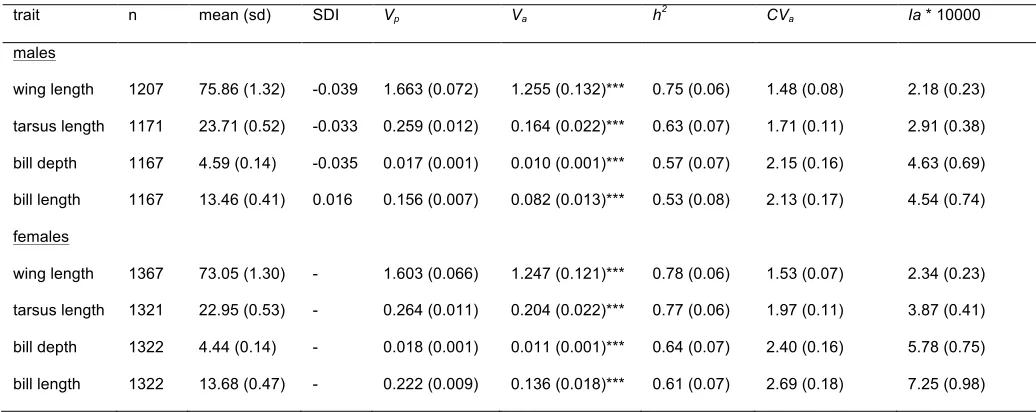
There was detectable additive genetic variance for all sex-specific traits (Table 1). The
440
proportion of phenotypic variance explained by additive genetic effects after accounting for fixed
441
effects (h2 ± SE) ranged from 0.53 ± 0.08 for male bill length to 0.78 ± 0.06 for female wing
442
length. In both sexes coefficients of variation (CVa) and mean-standardized additive genetic
443
variances (Ia) were lowest for wing and tarsus length and highest for bill length and width (Table
444
1).
445
446
Additive genetic covariances were generally positive, and significantly different from zero for
447
approximately half of the trait pairs (Table 2). Genetic correlations (rG ± SE) within each sex
448
were generally small, with the largest one being between tarsus length and bill depth in males
449
(0.508 ± 0.082). Genetic correlations between the sexes were similarly low, with the exception
450
of cross-sex genetic correlations between homologous traits, which were all large (> 0.8) and
451
not significantly smaller than one.
452
453
Male and female G matrices were significantly different from each other (Table 2, 2 × (LogL1
-454
LogL2) = 29.38, df = 10, p < 0.01). Genetic variances did not differ significantly between the
455
sexes (2 × (LogL1-LogL2) = 7.62, df = 4, p = 0.11). Genetic covariances and correlations were
456
always smaller in males than in females (Table 2), and these differences were statistically
significant (covariances: 2 × (LogL1-LogL2) = 26.16, df = 6, p < 0.001; correlations: 2 × (LogL1
-458
LogL2) = 27.94, df = 6, p < 0.001). The B matrix was not significantly asymmetric (2 × (LogL1
-459
LogL2) = 3.36, df = 6, p = 0.76).
460
461
Selection coefficients
462
We did not observe significant multivariate directional selection when including all traits from
463
both sexes as explanatory variables in a generalized linear model for either LRS (χ2 = 4.20, p =
464
0.38), longevity (χ2 = 5.71, df = 4, p = 0.22), or MRS (χ2 = 4.89, df = 4, p = 0.30). Similarly, we
465
did not observe significant sex × multivariate selection interaction for LRS (χ2 = 7.09, df = 4, p =
466
0.13) and MRS (χ2 = 2.00 , df = 4, p = 0.74). We did, however, observe a significant sex ×
467
multivariate selection interaction for longevity (χ2 = 14.04, df = 4, p < 0.01).
468
469
Unstandardized, mean, and variance standardized directional selection differentials and
470
gradients for LRS, longevity and MRS are presented in Table 3. Mean standardized directional
471
selection gradients for LRS ranged from -3.103 ± 1.927 for female tarsus length to 3.551 ±
472
1.314 for female bill depth. Only one selection gradient for LRS was statistically significant
473
(female bill depth, βu = 3.551 ± 1.314, p < 0.01) and this appeared to result mostly from
474
selection through longevity (βu = 2.661 ± 0.767, p < 0.001). While not statistically significant in
475
males, selection on bill length through longevity was notably different between the sexes (male
476
βu = 1.473 ± 0.867, p = 0.09, female βu = -1.493 ± 0.771, p = 0.05).
477
478
The angle between sex-specific vectors of mean-standardized selection gradients for LRS was
479
88.5° (95% CI = 31.5°-147.65°), meaning that multivariate selection in males and females was
480
neither predominantly parallel nor antagonistic. For longevity and MRS, the angle between
sex-481
specific vectors of mean-standardized selection gradients were 128.5° (59.5°, 156.4°) and
50.68° (20.43°, 145.82°), respectively. Overall, selection through longevity was therefore
(non-483
significantly) predominantly antagonistic between the sexes, while selection through MRS was
484
predominantly (non-significantly) parallel.
485
486
With the exception of bill depth in males, all point estimates for quadratic selection differentials
487
were negative. However, only those for female bill length were significant different from zero
488
(Appendix S1). No clear tendency emerged for quadratic and correlational selection gradients,
489
with statistical support being generally low (Appendix S2).
490
491
Selection responses
492
Predicted mean-standardized sex-specific responses when including and excluding the B matrix
493
are presented in Fig. 1. Point estimates for predictions based on LRS were largest for bill depth
494
and smallest for wing length. Selection through survival was expected to contribute most to the
495
evolution of bill depth, while selection through annual reproductive success was expected to
496
contribute most to the evolution of tarsus length. Patterns appeared to differ between the sexes
497
when setting all elements of B to zero. Most notably, bills were predicted to become deeper in
498
females but not in males. However, in general, predicted responses in males and females
499
became nearly identical once including B, suggesting little opportunity for the evolution of sexual
500
dimorphism given current multivariate selection and additive genetic (co)variances. Note,
501
however, that 95% confidence intervals generally overlapped between traits, fitness
502
components, and sexes.
503
504
Genetic variance for fitness
505
Together, sex-specific selection through LRS and G for the morphological traits considered here
506
accounted for genetic variance explaining less than 1% of the phenotypic variation in relative
507
fitness (𝑉!(!!𝐆!) = 0.0025, 95% CI = 0.0020, 0.0137; h2 = 0.0016, 95% CI = 0.0013, 0.0086,
Table 4). About 2/3 of this genetic variance was related to selection through MRS (𝑉!(!!𝐆!)=
509
0.0016, 95% CI = 0.0004, 0.0084), while the reminder was related selection through longevity
510
(𝑉!(!!𝐆!) = 0.0008, 95% CI = 0.0003, 0.0036). Sex-specific estimates are presented in Table 4.
511
512
The correlation between male and female genetic variance for relative fitness accounted for by
513
the set of morphological traits was -0.003 (95% CI = -0.83, 0.83). Longevity and MRS, when
514
considered in isolation, accounted for genetic variances in relative fitness that were negatively
-515
0.43 (95% CI = -0.86, 0.58) and positively 0.59 (95% CI = -0.78, 0.91) correlated between the
516
sexes, respectively. The ratio of 𝑉!(!!𝐆!)obtained while including B to 𝑉!(!!𝐆!) obtained while
517
excluding B was 1 (RB = 1.00, 95% CI = 0.27 – 1.73). Cross-sex genetic covariance therefore
518
did not impact 𝑉!(!!𝐆!) relative to a situation where traits were not genetically correlated
519
between the sexes. On the other hand, the presence of separate sexes, relative to a situation
520
where there would be no differences in selection and genetic architectures between the sexes,
521
resulted in a gender load of 50% (95% CI = 13, 86). Gender load estimates for longevity and
522
MRS were 68 % (95% CI = 25, 90) and 26% (95% CI = 8, 84), respectively.
523
524
525
Discussion
526
Significant additive genetic variance was detected for all traits, indicating that responses to
527
selection and genetic constraints were possible. Corresponding heritability estimates were
528
large, as is usually the case for morphological traits in birds (Merilä & Sheldon, 2001) including
529
previous estimates in Wytham Woods great tits obtained using a variety of methods (Gosler,
530
1987a; Robinson et al., 2013; Santure et al., 2015). Coefficients of variation (CVa) were also
531
typical of morphological traits in other species (Houle, 1992).
532
G matrices differed between the sexes, with covariances (and genetic correlations) being
534
consistently smaller in males than in females. Sex differences in G are relatively common and
535
have, for example, been documented in a number of vertebrates (Arnold & Phillips, 1999;
536
Jensen et al., 2003), invertebrates (Lewis et al., 2011; Rolff et al., 2005), and plants (Ashman,
537
2003; Campbell et al., 2011; McDaniel, 2005; Steven et al., 2007). Such differences are
538
important because they indicate that the sexes could respond differently to direct and indirect
539
selection. The larger genetic covariances in females suggest that genetic integration of
540
morphological traits may be greater in that sex. The reasons why that would be are unclear but
541
one possibility could be the presence of sex differences in correlational selection (McGlothlin et
542
al., 2005). Extra-pair paternities (EPP) may also have contributed to these patterns, a point we
543
return to below.
544
545
The evolution of sexual dimorphism depends on the structure of the B matrix, which includes
546
genetic covariance between homologous as well as non-homologous male and female traits
547
(Lande, 1980; Wyman et al., 2013). Genetic correlations between homologous male and female
548
traits were all very large, which was similar to previous findings for wing length and fledgling
549
mass in the same population (Garant et al., 2004; Robinson et al., 2013). Large genetic
550
correlations for traits exhibiting relatively low level of sexual dimorphism was consistent with the
551
tendency for cross-sex genetic correlations and sexual dimorphism to be negatively correlated
552
(Poissant et al., 2010). Combined with an absence of significant differences in additive genetic
553
variance between the sexes, our results suggests that the short-term evolution of sexual
554
dimorphism in Wytham Woods great tits may be limited for many aspects of morphology
555
(Lande, 1980). In contrast, genetic correlations between non-homologous traits were
556
comparatively small and at first sight appeared to play a smaller role in constraining the
557
evolution of sexual dimorphism; although assessing the constraining effect of individual genetic
558
correlations can be misleading (Walsh & Blows, 2009). Finally, for the traits considered here,
asymmetry of the B matrix (i.e. of its off-diagonal elements, Wyman et al., 2013) did not appear
560
to play a role in facilitating the evolution of sexual dimorphism.
561
562
The presence of a significant sex × multivariate selection interaction for longevity indicated that
563
aspects of morphology, or correlated traits, were under sex-specific directional survival
564
selection. However, this pattern was attenuated and no longer statistically significant once
565
combined with variation in MRS (i.e. when considering LRS). This illustrates how considering
566
various fitness components can increase knowledge about the biology of selection and
567
constraints, but also how individual fitness components, when treated in isolation, may lead to
568
erroneous evolutionary predictions. In the context of ISC, it also stresses out the need to
569
interpret and compare studies in the context of the fitness component used. For example, Tarka
570
et al. (2014) also studied ISC over morphological traits in a wild bird population using LRS but
571
they defined LRS as the total number of fledglings produced over an individual’s lifetime
572
whereas we defined LRS as the total number of recruits produced. While results from the two
573
studies are similar, they are therefore not entirely equivalent because the LRS metric used by
574
Tarka et al. (2014) did not include selection through survival to adulthood and sexual selection
575
(i.e. finding a mate) whereas the one used in herein did.
576
577
We detected significant directional selection for female bill depth when considering LRS, and
578
this pattern appeared to result primarily from viability selection. Bill morphology is a classic
579
example of a selected trait in birds, as is it closely tied to variation in the availability of different
580
food types. The strength of selection for female bill depth was relatively strong, as a βu of 3.55 is
581
larger than the 75% percentile for βu in natural populations (βu = 1.34) compiled by Hereford et
582
al. (2004). The selection gradient for female bill depth was also especially large considering that
583
our sample size was greater than most published studies to date and that large sample sizes
584
tend to yield smaller, more accurate, estimates (Hereford et al., 2004). In contrast, bill depth did
not appear to be under directional selection in males. Bill length, another important aspect of bill
586
morphology, appeared to be under sexually antagonistic viability (longevity) selection, but this
587
pattern was not mirrored by selection through MRS. As a consequence, evidence for sexually
588
antagonistic selection on bill length was attenuated when considering selection through LRS.
589
Sex differences in selection on bill morphology, believed to arise from sex differences in food
590
utilization, have been documented in other systems. For example, in a wild population of serin
591
(Serinus serinus), survival selection on bill morphology was directional in females but stabilizing
592
in males (Björklund & Senar, 2001). Male and female great tits are known to exploit different
593
dietary niches in Wytham Woods (Gosler, 1987a,b) and this could explain patterns documented
594
herein. Additional research on the drivers of sex-specific selection on bill morphology and
595
associated genetic constraints would be valuable; for example on the impact of spatial and
596
temporal heterogeneity in food availability and niche partitioning.
597
598
Extra-pair paternity (EPP) has been estimated at 12-13% in the study population (Firth et al.,
599
2015; Patrick et al., 2012) and these could have affected selection coefficients and quantitative
600
genetic parameters estimates. This situation is similar to other studies where molecular
601
parentage analyses are not routinely conducted, such as in humans (e.g. Bolund et al., 2013;
602
Stearns et al., 2012). EPP introduce errors in male LRS estimates, which may unduly reduce
603
covariance between LRS and trait variation in that sex. EPP is also expected to limit phenotypic
604
resemblance between offspring and their (social) father as well as other relatives (e.g. paternal
605
grand-parents), which could reduce additive genetic variance and heritability of both male and
606
female traits estimated from an animal model but more so for male traits (Brommer et al., 2005;
607
Brommer et al., 2007; Charmantier & Réale, 2005; Jensen et al., 2003; Morrissey et al., 2007).
608
Reduced phenotypic resemblance between offspring and paternal relatives could also reduce
609
genetic covariance within and between the sexes. We would expect such a bias to be most
610
pronounced for male-specific genetic covariances, followed by cross-sex and female-specific
covariances. Larger covariances in females compared to males were consistent with this
612
predicted pattern. However, it is worth noting that sex differences in genetic correlations were
613
substantial, and that Morrissey et al. (2007) found that, for the most part, genetic correlations
614
are usually unbiased by pedigree errors because covariances and variances are usually
615
underestimated in similar proportions. The large differences between male and female genetic
616
correlations therefore suggest that sex differences in quantitative genetic parameters were
617
unlikely due to EPP alone. Nonetheless, the potential for EPP to bias estimates means that any
618
downstream sex differences in evolutionary predictions should be interpreted with caution.
619
620
In this study we have quantified the evolutionary consequences of ISC over a set of
621
morphological traits in a population of great tits by estimating the impacts of sex-specific
622
selection and genetic variance on the population’s rate of adaptation. At face value, a gender
623
load of 50% for a set of traits exhibiting little sexual dimorphism appeared substantial. In
624
comparison, in a similar study in Red Deer (Cervus elaphus) by Walling et al. (2014), gender
625
load for a set of life history traits was estimated at 27.5% (calculated from their multivariate
626
evolvability ratio of 1.45). However, additional studies where a similar approach is applied will
627
be needed to reach conclusions on the relative importance of ISC quantified here and by
628
Walling et al. (2014). Estimates were also arguably imprecise, but since the current study and
629
the one of Walling et al. (2014) were based on two of the world’s largest datasets for wild
630
pedigreed populations, similarly or even less precise results are to be expected as researchers
631
work toward quantifying the impacts of ISC in other systems. This is perhaps not surprising
632
given that the estimation of genetic covariances is known to require large sample sizes (Lynch,
633
1999) and that selection analyses in wild populations are often underpowered (Hersch &
634
Phillips, 2004). In that context, the joint publication of B matrices and sex-specific selection
635
gradients should be encouraged, even in the absence of significant results, as compiling results
636
from a large number of studies will be necessary to contextualize results and gain a broader
understanding of the importance of ISC in constraining contemporary evolution in natural
638
populations (Cox & Calsbeek, 2009; Poissant et al., 2010; Wyman et al., 2013).
639
640
Acknowledgments
641
We thank the many people and funding sources, too numerous to list here, that have
642
contributed to the Wytham Woods great tit project over the years. We would also like to thank
643
Anna Santure, Mark Adams and Matt Robinson for constructive discussions during the
644
formulation and execution of this work. Matthew Wolak and anonymous referees provided
645
valuable feedback on previous versions of this manuscript. This work was part of JP’s
post-646
doctoral research at the University of Sheffield funded by the Natural Sciences and Engineering
647
Council of Canada (NSERC) and a Marie Curie International Incoming Fellowship. JP was
648
supported by a Leverhulme Trust Early Career Fellowship. MBM was supported by a Royal
649
Society University Research Fellowship.
650
651
652
653
654
655
656
657
658
659
660
661
662
Table 1. Number of individuals, raw trait means (in millimetres), sexual dimorphism index (SDI)
664
and univariate quantitative genetic parameters for sex-specific morphological traits in a wild
665
population of great tits. Phenotypic variances after having accounted for fixed effects (Vp) and
666
additive genetic variances (Va) were estimated using a multivariate animal model. Heritability (h2
667
= Va / Vp), coefficient of variation (CVa) and mean-standardized additive genetic variance (Ia) are
668
also presented. Standard errors are presented in parentheses. Statistical significance of Va was
669
tested using likelihood ratio tests.
670
trait n mean (sd) SDI Vp Va h2 CVa Ia * 10000
males
wing length 1207 75.86 (1.32) -0.039 1.663 (0.072) 1.255 (0.132)*** 0.75 (0.06) 1.48 (0.08) 2.18 (0.23)
tarsus length 1171 23.71 (0.52) -0.033 0.259 (0.012) 0.164 (0.022)*** 0.63 (0.07) 1.71 (0.11) 2.91 (0.38)
bill depth 1167 4.59 (0.14) -0.035 0.017 (0.001) 0.010 (0.001)*** 0.57 (0.07) 2.15 (0.16) 4.63 (0.69)
bill length 1167 13.46 (0.41) 0.016 0.156 (0.007) 0.082 (0.013)*** 0.53 (0.08) 2.13 (0.17) 4.54 (0.74)
females
wing length 1367 73.05 (1.30) - 1.603 (0.066) 1.247 (0.121)*** 0.78 (0.06) 1.53 (0.07) 2.34 (0.23)
tarsus length 1321 22.95 (0.53) - 0.264 (0.011) 0.204 (0.022)*** 0.77 (0.06) 1.97 (0.11) 3.87 (0.41)
bill depth 1322 4.44 (0.14) - 0.018 (0.001) 0.011 (0.001)*** 0.64 (0.07) 2.40 (0.16) 5.78 (0.75)
bill length 1322 13.68 (0.47) - 0.222 (0.009) 0.136 (0.018)*** 0.61 (0.07) 2.69 (0.18) 7.25 (0.98)
* p < 0.05, ** p < 0.01, *** p < 0.001.