Invariant object recognition : biologically plausible and machine learning approaches

(1)

warwick.ac.uk/lib-publications

A Thesis Submitted for the Degree of PhD at the University of Warwick

Permanent WRAP URL:

http://wrap.warwick.ac.uk/83167

Copyright and reuse:

This thesis is made available online and is protected by original copyright.

Please scroll down to view the document itself.

Please refer to the repository record for this item for information to help you to cite it.

Our policy information is available from the repository home page.

(2)

Invariant Object Recognition

Biologically Plausible and Machine Learning

Approaches

by

Leigh Robinson MSc, MEng.

Submitted to the University of Warwick for the degree of

Doctor of Philosophy

Complexity Science Doctoral Training Centre

&

Department of Computer Science

(3)

(4)

List of Figures

Figure 2.1 Caricature of the regions of the visual cortex and their major interconnections. The dorsal areas, MT (medial temporal), MST (medial superior temporal) and FST (fundus of superior temporal suculus) seem to be primarily concerned with motion and the location of objects. The red (bold) feed-forward ventral pathway is where the majority of object recognition processes are thought to take place. Adapted from Gross et al.(1993) · · · 6

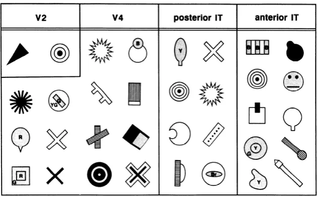
Figure 2.2 Examples of features identified byKobatake and Tanaka (1994) grouped by

the region of the visual hierarchy. Note that the stimuli become more visually complex as you traverse the ventral stream. (AfterKobatake and Tanaka(1994)). _{· · · ·} 8

Figure 2.3 Examples of various symmetric (bottom) and anti-symmetric (top) Gabor

filters at various scales (horizontal progression). · · · 11

Figure 2.4 Gabor filters of various scales and orientations are applied to a sample image. 11

Figure 3.1 Convergence in the visual system. Right – as it occurs in the brain. V1, visual cortex area V1; TEO, posterior inferior temporal cortex; TE, inferior temporal cortex (IT). Left – as implemented in VisNet. Convergence through the network is designed to provide fourth layer neurons with information from across the entire input retina. · · · 22

Figure 3.2 Sketch of the HMAX model of invariant object recognition (Riesenhuber and

Poggio 1999a,2000a). The model includes layers of ‘S’ cells which perform template matching

(solid lines), and ‘C’ cells (solid lines) which pool information by a non-linear MAX function to achieve invariance (see text). (After (Riesenhuber and Poggio 1999a)) · · · 29

Figure 3.3 Example images from the Caltech256 database for two object classes, hats

and beer mugs. · · · 33

Figure 3.4 Performance of HMAX and VisNet on the classification task (measured by the

(9)

List of Figures

Figure 3.5 Top: Firing rate of two output layer neurons of VisNet, when tested on two of the classes, hats and beer mugs, from the Caltech 256. The firing rates to 10 untrained (i.e. testing) exemplars of each of the two classes are shown. One of the neurons responded more to hats than to beer mugs (solid line). The other neuron responded more to beer mugs than to hats (dashed line). Middle: Firing rate of two C2 Tuned Units of HMAX when tested on two of the classes, beer mugs and hats, from the Caltech 256. Bottom: Firing rate of a View Tuned Unit of HMAX when tested on two of the classes, hats (solid line) and beer mugs (dashed line), from the Caltech 256. The neurons chosen were those with the highest single cell information that could be decoded from the responses of a neuron to 10 exemplars of each of the 2 objects (as well as a high firing rate) in the cross-validation design. · · · 37

Figure 3.6 Example images from the two object classes within the ALOI database, (a)

293 (light bulb) and (b) 156 (clock). Only the 45 degree increments are shown. · · · 39

Figure 3.7 Performance of VisNet and HMAX C2 units measured by the percentage of

images classified correctly on the classification task with 8 objects using the Amsterdam Library of Images dataset and measurement of performance using a pattern association net-work with one output neuron for each class. The training set consisted of 4 views of each object spaced 90 degrees apart; or 9 views spaced 40 degrees apart; or 18 views spaced 20 degrees apart. The test set of images was in all cases a cross-validation set of 18 views of each object spaced 20 degrees apart and offset by 10 degrees from the training set with 18 views and not including any training view. The 10 best cells from each class were used to

measure the performance. Chance performance was 12.5% correct. · · · 40

Figure 3.8 Top: Firing rate of one output layer neuron of VisNet, when trained on 8

objects from the Amsterdam Library of Images, with 9 views of each object spaced 40 degrees apart. The firing rates on the training set are shown. The neuron responded to all 9 views of object 4 (a light bulb), and to no views of any other object. The neuron illustrated was chosen to have the highest single cell stimulus-specific information about object 4 that could be decoded from the responses of the neurons to all 72 exemplars shown, as well as a high firing rate to object 4. Middle: Firing rate of one C2 Unit of HMAX when trained on the same set of images. The unit illustrated was that the highest mean firing rate across views to object 1 relative to the firing rates across all stimuli and views. Bottom: Firing rate of one View Tuned Unit (VTU) of HMAX when trained on the same set of images. The unit illustrated was that the highest firing rate to view 1 of object 1. · · · 42

(10)

List of Figures

Figure 3.9 Top: Firing rate during cross-validation testing of one output layer neuron of VisNet, when trained on 8 objects from the Amsterdam Library of Images, with 9 exemplars of each object with views spaced 40 degrees apart. The firing rates on the cross-validation testing set are shown. The neuron was selected to respond to all views of object 4 of the training set, and as shown responded to 7 views of object 4 in the test set each of which was 20 degrees from the nearest training view, and to no views of any other object. Middle: Firing rate of one C2 Unit of HMAX when tested on the same set of images. The neuron illustrated was that the highest mean firing rate across training views to object 1 relative to the firing rates across all stimuli and views. The test images were 20 degrees away from the test images. Bottom: Firing rate of one View Tuned Unit (VTU) of HMAX when tested on the same set of images. The neuron illustrated was that the highest firing rate to view 1 of object 1 during training. It can be seen that the neuron responded with a rate of 0.8 to the two training images (1 and 9) of object 4 that were 20 degrees away from the image for which the VTU had been selected. · · · 43

Figure 3.10 Similarity between the outputs of the networks between the 9 different views of 8 objects produced by VisNet (top), HMAX C2 (middle), and HMAX VTUs (bottom) for the Amsterdam Library of Images test. Each panel shows a similarity matrix (based on the cosine of the angle between the vectors of firing rates produced by each object) between the 8 stimuli for all output neurons of each type. The maximum similarity is 1, and the minimal similarity is 0. · · · 44

Figure 3.11 Examples of images used in the scrambled faces experiment. Top: Two of

the 8 faces in 2 of the 5 views of each. Bottom: examples of the scrambled versions of the faces. · · · 45

Figure 3.12 Top. Effect of scrambling on the responses of a neuron in VisNet. This

VisNet layer 4 neuron responded to one of the faces after training, and to none of the other 7 faces. The neuron responded to all the different view exemplars 1–5 of the unscrambled face (exemplar normal). When the same neuron was then tested with the randomly scrambled versions of the same face stimuli (exemplar scrambled), the firing rate was zero. Bottom. Effect of scrambling on the responses of a neuron in HMAX. This View Tuned Neuron of HMAX was chosen to be as discriminating between the 8 face identities as possible. The neuron responded to all the different view exemplars 1–5 of the unscrambled face. When the same neuron was then tested with the randomly scrambled versions of the same face stimuli, the neuron responded with similarly high rates to the scrambled stimuli. · · · 47

Figure 3.13 View invariant representations of cups. The two objects, each with four

views. · · · 48

Figure 3.14 Top. View invariant representations of cups. Single cells in the output

(11)

List of Figures

Figure 4.1 This figure shows the appearance of the gradients that are computed on the

first iteration when relabelling an image from class 10, to class 348. Notice that the for the gradient passed through the sgn function (4.1(b)) the values are much more spread out spatially, and each colour channel are either -1/255, 0 or 1/255. This stops "hot spots" appearing in the image from the large clustered values apparent in 4.1(a) when used in the gradient descent. · · · 69

Figure 4.2 Examples of class relabelling on GoogLeNet. Left: Original images that are

correctly classified as ’Shih-Tzu’ and ’Half-track’. Right: relabelled images such that the classification output is reversed - i.e the ’Shih-Tzu’ is now strongly classified as ’Half-track’ and vice-versa. Centre: Pixel differences multiplied by 10 and scaled to mean-level for visibility. The distortion introduced in the top relableling was 0.00864 and the bottom 0.00712. These are a random pair of images taken from the above classes that were chosen to be qualitatively "maximally different". As we show in Section 4.3.1 relabelling is not sensitive to the initial or target class. · · · 70

Figure 4.3 The class probabilities for each of the four images in Fig 4.2. Notice that

after relabelling the uncertainty is also reduced. · · · 71

Figure 4.4 These figures show a random gaussian image (4.4(a)) and the same image after

being re-labeled to class 348 (4.4(b)). The bottom two graphs show the class probabilities before and after the relabelling process. The distortion introduced in this relabelling process was 0.03 - which is much higher than typically required to relabel natural images. · · · 72

Figure 5.1 Example of applying dropout to a fully connected neural network · · · 74

Figure 5.2 Left: MNIST training time for three layer networks (log scales) on an NVIDIA

GeForce GTX 780 graphics card. Right: Percentage reduction in training times moving from no dropout to batchwise dropout. The time saving for the 500N network with minibatches of size 100 increases from 33% to 42% if you instead compare batchwise dropout with inde-pendent dropout. · · · 77

Figure 5.3 Dropout networks trained using a restricted the number of dropout patterns

(each◊is from an independent experiment). The blue line marks the test error for a network

with half as many hidden units trained without dropout. · · · 79

Figure 5.4 Results comparing the performance of independent and batchwise dropout on

the CIFAR-10 dataset using fully-connected networks of different sizes. · · · 80

Figure 5.5 Results comparing the performance of independent and batchwise dropout

on the artificial dataset using networks of different sizes. 100 classes each corresponding to noisy observations of a one dimensional manifold in{0,1}1000. · · · 81

Figure 5.6 MNIST test errors, training repeated three times for both dropout methods. · 82

Figure 5.7 CIFAR-10 results using a convolutional network with dropout probability

p_œ(0,0.4). Batchwise dropout produces a slightly lower minimum test error. _{· · · ·} 83

Figure 6.1 The general structure of a Restricted Boltzmann Machine (RBM) is comprised

of a bipartite graph of nodes which are labelled visible, v and hidden h. The pair-wise

interactions of nodes between layers is defined by a connectivity matrix,W. · · · 88

(12)

List of Figures

Figure 6.2 This diagram shows one step contrastive divergence (CD) learning. At time

t= 0 we sample the states of the hidden units having clamped the visible units to an exemplar

in the dataset. At timet= 1 we then sample the visible units given the previous hidden node

samples which in turn allows a re-sampling of the hidden units. This iterative process can be computed more times to get better estimates, but commonly one is sufficient for gradient estimates good enough to learn with. · · · 91

Figure 6.3 The MNIST handwritten digit database. The clean images (a) and the four

corrupted versions: random noise (b), rotations (c), occlusions (d) and translations (e). · · · 93

Figure 6.4 Error rates of DBN models with various receptive field sizes when tasked to

classify MNIST images corrupted with increasing amounts of noise. Notice that while the fully connected model (image sized receptive fields - 28x28) very quickly degrades to random chance, the others do not.· · · 94

Figure 6.5 Error rates of LCDBN models with various receptive field sizes when tasked

to classify MNIST images corrupted with translations (a), rotations (b) and occlusions (c). Unlike with noise corruption (Fig 6.4) in these cases local connectivity does not seem to offer any benefits. · · · 95

Figure 6.6 Example images drawn from four of the classes from the CIFAR-10 dataset.

The rows correspond to the classes (from the top)airplane,automobile,bird, and cat. Each image is 32◊32 in size. · · · 96

Figure 6.7 Some exemplar receptive fields of units in the first (a) and second layer (b)

of a LCDBN trained on the CIFAR-10 dataset with 11x11 Gaussian receptive fields. · · · 97

Figure 6.8 Orientation maps computed for the first (a) and second (b) layers of a 11x11

(13)

List of Figures

(14)

List of Tables

Table 3.1 VisNet dimensions · · · 22

Table 3.2 Sigmoid parameters · · · 23

Table 3.3 Lateral inhibition parameters · · · 24

Table 3.4 Layer 1 connectivity · · · 26

(15)

List of Tables

(16)

Acknowledgements

I would first like to thank the most important person in the world: my wife and best friend, Kelli. Her support over the course of this PhD has been nothing short of fantastic and every day that passes I am reminded how lucky I am to be going through life with her by my side. It absolutely goes without saying that I would not be the person I am today without her help and encouragement. Thanks, toots!

I would of course also like to thank my supervisors, Prof. Edmund Rolls and Dr. Ben Graham. Edmund, has consistently gone above and beyond in his duties as a supervisor and his exceptional work ethic will be an enduring inspiration. Ben was likewise always willing to entertain discussions that would run on for hours longer than scheduled, frequently leaving me reinvigorated for the project. So thank you Edmund. Thank you Ben. It was very much appreciated.

It would be remiss of me to not thank all the people within the Complexity Department who have supported my studies and the EPSRC for a generous stipend that made this journey financially viable.

(17)

List of Tables

(18)

Publications

1. Robinson, L. & Rolls, E. T., 2015. Invariant Visual Object Recognition: Biologically Plausible Approaches. Biological Cybernetics, 2015, 109(4-5):505-35.

2. Robinson, L. & Graham, B., 2015. Confusing Deep Convolutional Networks by Relabelling.

arXiv Preprint, arXiv:1510.06925.

(19)

List of Tables

(20)

Abstract

Understanding the processes that facilitate object recognition is a task that draws on a wide range of fields, integrating knowledge from neuroscience, psychology, computer science and mathematics. The substantial work done in these fields has lead to two major outcomes: Firstly, a rich interplay between computational models and biological experiments that seek to explain the biological pro-cesses that underpin object recognition. Secondly, engineered vision systems that on many tasks are approaching the performance of humans.

This work first highlights the importance of ensuring models which are aiming for biological rele-vance actually produce biologically plausible representations that are consistent with what has been measured within the primate visual cortex. To accomplish this two leading biologically plausible models, HMAX and VisNet are compared on a set of visual processing tasks.

(21)

List of Tables

(22)

(23)

(24)

Introduction

The research described in this thesis aims to investigate both biologically plausible and machine learning approaches to invariant visual object recognition.

This thesis first summarises the substantial work that has been done trying to understand the bio-logical mechanisms behind invariant object recognition and the attempts to build both explanatory models and specific engineering solutions to solve vision tasks. Specific emphasis is placed upon the interdisciplinary nature of this work, with successful models integrating knowledge across neu-roscience, psychology, computer science and mathematics.

The thesis is then split into two parts; the first highlighting the importance of biologically plau-sible models producing representations that are consistent with that measured from within the primate visual cortex. The aim of these models isn’t to engineer high performance on a particular vision task, but rather investigate how the brain accomplishes the task. This interplay between the experimental evidence and computational modelling allows for the refinement of quantitative theories of vision that seek to explain how the cortical structures might be computing useful repre-sentations for vision. Specifically, the two leading biologically plausible models of invariant object recognition, VisNet (Rolls 2008b,2012b) and HMAX (Riesenhuber and Poggio 1999b,2000b;Serre

et al. 2005). The aim of this comparison is to investigate which of these two approaches better

account for what is found neurophysiologically in the primate brain areas involved in invariant visual object recognition.

The second part focuses on extending models that do not explicitly seek to model any of the biological processes, but rather solve a particular vision task with the guiding principle being that of increased performance rather than biological plausibility. This second half focuses on extending the Deep Belief Network model (Hinton 2009;Hinton et al. 2006) with a local connectivity constraint, exploring a new method for creating adversarial exemplars (Goodfellow et al. 2015;Szegedy et al. 2014) and an efficient way to apply dropout (Hinton et al. 2012) without losing model accuracy.

The contrast of these approaches at even a high level is both interesting and revealing. One funda-mental difference is that the majority of biologically plausible approaches have strived to account for how an individual member of a class, for example a particular person, can be recognised in-variantly with respect to various transforms such as view, pose, etc. In contrast machine learning approaches to vision have tended to attempt to solve a slightly different problem, that of the cate-gorisation of individual exemplars into broad classes such as cars, dogs, cats, etc. The distinction between the identification and classification problem might on the surface seem trivial and perhaps unnecessary, but it is important to point out that the neurophysiology has consistently shown the representations built at the highest levels of the visual cortex are that of identities and not classes (Rolls 2008b).

(25)

Chapter 1. Introduction

learned is provided VisNet (Rolls 2008b, 2012b). In contrast many machine learning approaches tend to use less well posed training sets in that they typically comprise very large numbers of exemplars of many categories of object, with no attempt to provide a systematic set of different views of each object to provide a basis for view-invariant object recognition.

Some of the biologically plausible approaches have used semi-supervised learning, which has been provided a mechanism to attempt to learn from the temporal continuity that reflects natural image statistics (Rolls 2008b, 2012b). This assumes that typically humans and other primates inspect an object for a short period while it undergoes transforms, for example rotation into different views, scale change, etc. The eyes then move to a different object in which transforms of the new object may then also be seen for a short time period. Some biologically plausible approaches such as VisNet explicitly take advantage of these statistics to help the system learn which images

correspond to the transforms of an individual object (Rolls 2008b, 2012b). In contrast most

machine learning approaches that are unsupervised, only identify categories based on similarities of image statistics of large numbers of exemplars of many categories of object.

Partly for these reasons comparing these two types of approach may enable strengths of each type of approach to be combined to enable new progress to be achieved.

(26)

Modelling Vision: Object

Recogni-tion

Introduction

In this chapter the basic results from neurophysiology that are thought to underpin the biological basis of vision, and specifically object recognition are reviewed. It shall be seen that this body of work strongly suggests that at least for object recognition, the visual cortex acts as a hierarchical series of feature extraction and combination stages. Before a detailed discussion of how these results are integrated into biologically inspired computational models of object recognition a brief discussion of other potential psychophysical and computational approaches will be undertaken. A comprehensive review of the neurophysiology and computational approaches can be found in (Rolls

and Deco 2002;Ullman 1996).

Neurophysiology of Vision

The human visual system is a remarkably powerful system that is perhaps capable of discriminating between tens of thousands of distinct objects (Biederman 1987). Detailed and accurate knowledge of the architecture and circuitry involved in the visual cortex is required to inform biologically sound computational models. The invasive nature of traditional measurement techniques inevitably mean that the bulk of our knowledge has been gathered from non-human primates. The remainder of this section will describe some of the fundamental neurophysiology that has been uncovered about the visual cortex with particular attention to mechanisms that are implicated in object recognition.

Dorsal and ventral streams

The first place to begin when explaining the known neurophysiology, is with that of the high level cortical organisation involved with the processing of visual stimuli. The visual pathway has been described as being made up of two primary pathways, named the dorsal and ventral stream (see Fig. 2.1).

The dorsal stream starts in the primary visual cortex (V1), from where it proceeds to areas V2 and the middle temporal area (MT) before ending up in the posterior parietal cortex. The dorsal stream is often characterised as the ‘where’ or ‘how’ pathway and is strongly associated with the perception of motion, the positions of objects in the visual field and feedback control of the eyes

(27)

Chapter 2. Modelling Vision: Object Recognition

V1

V2

V3

V4

IT

MT

MST, FST

Other Dorsal Areas

Ventral

Stream

LGN

“What”

Dorsal

Stream

“Where”

Figure 2.1: Caricature of the regions of the visual cortex and their major inter-connections. The dorsal areas, MT (medial temporal), MST (medial superior temporal) and FST (fundus of superior temporal suculus) seem to be primar-ily concerned with motion and the location of objects. The red (bold) feed-forward ventral pathway is where the majority of object recognition processes are thought to take place. Adapted fromGross et al.(1993)

The split of the visual pathway into this dichotomy is known as the ‘two-streams hypothesis’ and was first proposed byUngerleider and Mishkin (1982). Significant research supports the idea of two functionally distinct processing streams within the primate visual system (Baizer et al. 1991;

Felleman and Van Essen 1991; Livingstone and Hubel 1988, 1987; Maunsell and Newsome 1987;

Van Essen et al. 1992a). While this split hierarchy is well established the two pathways are not

completely independent as can be seen on Fig. 2.1. There are significant cross pathway connections

(Ungerleider and Haxby 1994; Van Essen et al. 1992a). The remainder of this section will limit

itself to the cortical structures that dominate the ventral stream since the focus of this work is object recognition processes.

When light enters the back of the eye, it stimulates light sensitive cells on the retina. These cells effectively transduce the incoming light into an electric form, that is carried by the nervous system. The retina itself comprises of quite complex neural circuitry, the retinal ganglion cells already do some processing of the visual information before relaying it via the optic nerve to the lateral geniculate nucleus (LGN) in the thalamus before again relaying it to the occipital lobe -the first area of -the visual cortex, V1 (Callaway 2004).

Primary visual cortex - V1

The V1 area was first systematically studied with the ground breaking work ofHubel and Wiesel

(1962, 1968a). Their work cemented the ideas that individual neurons in V1 have a region, or

receptive fieldin the visual field that generates a maximum response and that these receptive fields

vary somewhat continuously over space forming a retinotopic map (Talbot and Marshall 1941).

This map is not an isometric mapping, there is significantly more cortical area devoted to that of the central portions of the visual field. Neurons within V1 can be classified into three groups: simple

(28)

cells, complex cells and hypercomplex cells. The simple cells have a centre surround receptive field with elongated excitatory and inhibitory areas at a specific angle - which makes them sensitive to oriented luminous edges (i.e are edge/bar detectors) in the visual field (Hubel and Wiesel 1962). The complex cells, much like the simple cells have receptive fields that act as edge detectors but they respond over a larger region of the visual field - they have a degree of invariance to position (but usually not orientation) (Hubel and Wiesel 1962). The hypercomplex cells exhibit even more complex receptive fields, seemingly only strongly responding to lines of a specific orientation moving in a specific direction and only if the stimulus is under a certain length (Wiesel and Hubel 1965). These properties have led to the idea that (at least in regard to static images) V1 functions in some ways analogous to a filter bank of oriented edge/bar detectors - the operation of which is

commonly modelled by Gabor functions (Carandini et al. 2005;Daugman 1988b;Teich and Qian

2006). Other distinguishing properties of V1 are known, such as ocular dominance regions (LeVay et al. 1980) and color specific processing regions (blobs) (Livingstone and Hubel 1988).

Visual areas V2 & V4

V2, or the ‘prestriate cortex’ has been shown to build upon the responses of neurons in V1, with evidence of specific selectivity to combinations of orientations from V1 (Anzai et al. 2007). V2 physiology is characterised by dark bands of thick and thin stripes, with lighter regions between

them called ‘interstripes’ (Livingstone and Hubel 1982). Neurons within the thick bands have

been named ‘form’ cells and are strongly orientation and direction sensitive, much like complex cells of V1. Neurons within the thin bands show no orientation sensitivity, but are sensitive to particular colours and so are thought to be principally connected to ‘blob’ cells from V1 (

Living-stone and Hubel 1988). V2 has been implicated in the perceptual phenomena of illusory contours,

withPeterhans and von der Heydt(1989) reporting significant numbers of neurons in this region

responding to contours extending across gaps.

V4 region is thought to be made up of at least receives input primarily from the thin and interstripe cells of V2 and as such are heavily implicated in colour (Dubner and Zeki 1971) and orientation

(Desimone and Schein 1987). V4 is the first area of the ventral stream where strong attentional

(top down) mechanisms can be measured - the receptive field sizes contract at the position being attended to (Moran and Desimone 1985;Reynolds et al. 1999;Schiller 1994). The receptive fields of neurons in V4 are significantly larger than that of V1 and V2, but smaller than those in the nex area, the inferior temporal cortex (IT) (Kobatake and Tanaka 1994).

Inferior temporal cortex - IT

The inferior temporal cortex (IT) is thought to be the final area of the brain that is dedicated to exclusively processing visual information and completes the hierarchy through the ventral stream - taking the majority of its input from V4 (Ungerleider and Haxby 1994;Ungerleider and Mishkin 1982).

Cells within IT tend to preferentially respond to complex visual stimuli (Gross et al. 1972, 1993;

Tanaka 1996). Indeed many neurons show no response to simple oriented edges (Kobatake and

Tanaka 1994). Furthermore the responses to complex stimuli are robust to transformations

(29)

1993; Kobatake and Tanaka 1994; Perrett et al. 1982; Rolls 1991; Rolls et al. 1994). The

build-ing of these invariant responses (neurons that fire strongly for a given stimuli regardless of the transformation) is fundamental to the task of object recognition (Logothetis et al. 1995).

RESPONSES TO COMPLEX OBJECT FEATURES 865

v2 v4 posterior IT anterior IT

) @%tzuY

FIG. 11. Examples of the complex criti-

cal features in the 4 regions. YG, yellow green; Br, brown.

posterior IT, but not in V2, responded maximally to particular complex object features, as did cells in anterior IT. 2) The selectivity of the cells in anterior IT was generally dis- tinctive, but cells with selectivity of varying distinctiveness intermingled in V4 and posterior IT. Although the critical features for cell responses have previously been examined in anterior IT (Desimone et al. 1984; Gross et al. 1972; Tanaka et al. 199 1 ), posterior IT, and V4 (Tanaka et al. 199 1 ), the distinctiveness of the selectivity, which turned out to be a key issue in posterior IT and V4, was quantified for the first time in the present study. A prominent increase in the size of the receptive fields from posterior IT to anterior IT was also observed, but this is rather confirmation of the previous results (Desimone and Gross 1979; Tanaka et al. 1991).

One of the authors previously reported that only 2% of responsive cells in V4 and 12% of those in posterior IT selectively responded to complex object features (Tanaka et al. 199 1). In the present study we found that greater pro- portion of cells in these areas, i.e., 38% in V4 and 49% in posterior IT (S,,,/MAX < 0.75, Fig. lo), required complex features for their maximal activation. We found that many cells in these areas showed moderately strong responses to some simple stimulus as well as the maximum response to the complex critical feature. Such cells might be classified as “primary cells” in the previous study, in which the classification was performed mostly qualitatively by hearing discharges, because they responded to some simple stimuli. Also, the introduction of a special computer graphic system in the present experiments facilitated the exploration of effective stimuli and the quantitative comparison of the effectiveness of different stimuli.

Earlier, Tanaka et al. ( 1986) reported the presence of cells in the prelunate gyrus that specifically responded to “stimuli with an irregular internal structure or texture.” Recently, Gallant et al. ( 1993) reported that a sizable pro- portion of V4 cells responded to concentric or hyperbolic patterns more strongly than to straight gratings of any orientation. Some of our critical features in V4 and posterior IT were similar to the concentric or hyperbolic patterns, but our critical features were more divergent.

At what point is the selectivity to complex object features attained? The distribution of S&MAX, the ratio of the maximum response to simple stimuli to the total maximum response of the individual cells, showed the most prominent changes from V2 to V4 and from posterior IT to anterior IT (Fig. 10). This might appeal as evidence that integration of features advances in V4 and anterior IT. However, there is no reason to assume that the sample of cells represented outputs of the areas. Rather, the cells, which were randomly sampled at various depth, should have included cells at various stages of the local networks. The ratio S ,,,/MAX showed the greatest intra-area1 variety in posterior IT and V4 (Figs. 8 and 10). If we assume that the selectivity is determined in local networks but not in corticocortical connections, a random sample of cells from one such local network should include cells with varying complexity of selectivity. A cell located close to the input end should respond maximally to some primary feature that corresponds to a component of the final feature, a cell located close to the output end should respond rather selectively to the final integrated feature, and a cell located at the middle should show an intermediate property. The sam- plings from V4 and posterior IT but not those from anterior IT fulfilled this condition. The initial assumption is plausible on the basis of the complicated intrinsic connections in the local regions of the cerebral cortex (Lorente de No 1938; Lund 1988). The computational power of these complicated local circuitries should be greater than that of the one-step corticocortical connections. Thus we suggest that signals of primary features are integrated to form complex features in local networks of V4 and posterior IT.

The receptive fields of cells in V4 and posterior IT were smaller than those of cells in anterior IT. These small receptive fields are advantageous for integration of components because activities of cells with small receptive fields provide information regarding the position of the components, which may be necessary for the integration. If the integration occurred with large receptive fields such as those in anterior IT, there should be some sophisticated mechanism to register positional relationship between the components. On the other hand the large receptive fields in anterior IT

Figure 2.2: Examples of features identified by Kobatake and Tanaka (1994) grouped by the region of the visual hierarchy. Note that the stimuli become more visually complex as you traverse the ventral stream. (AfterKobatake and Tanaka(1994)).

The neurophysiological evidence of the preceding section strongly suggests that the ventral process-ing stream tends to be organised to integrate information in a hierarchical manner. The preferred stimuli of neurons becomes more complex as you move from area to area (see Fig. 2.2) (Kobatake

and Tanaka 1994), the receptive fields increase significantly until they encompass upwards of 50 deg

or more (Boussaoud et al. 1991;Perrett and Oram 1993;Rolls 1992) and typically encompass the foveal region (Gross et al. 1972). Finally the degree of invariance to transformations that the preferred stimuli can undergo increases. These architectural features will play a significant part in the development of computational models of object recognition.

Computational Models of Vision

The approaches to constructing computational models of object recognition can be broadly classi-fied into two groups, each with different motivations and goals. The first adopts the perspective of computational neuroscience and utilise computational modelling as a tool to refine the under-standing of complex experimental neurological evidence towards that of a cohesive theory of vision. In keeping with this aim these types of models are thus heavily constrained to operate in a man-ner which is biologically plausible. In contrast the second group follow a more machine learning, engineering led philosophy that eschews the strict restriction of biology and instead embarks on an undertaking to simply engineer a vision system that for a given specific task can by various metrics perform well - i.e mimic the human visual system, rather than explain.

The variety of computational models that have arisen can be similarly grouped into two loose categories: structural models and view models.

[image:29.595.112.428.162.358.2]

(30)

Structural Models

One approach to modelling object recognition might be to assume that objects can be represented by a decomposition of the object into simple component parts and within such an object referenced representation a hierarchical spatial relationship between components can be established. Several models exhibiting such a decomposition can be thought to stem from the influential work of David

Marr (Marr 1982; Marr and Nishihara 1978). The chief motivation of these models seems to be

that invariant object recognition is an easier task if the object has first been reduced to a structural description. With Marr suggesting that this decomposition of objects not only results in an explicit 3D representation, but that recognition occurs in a fundamentally bottom-up hierarchical fashion (Marr 1982). Subsequent extensions of this idea were made byBinford(1981);Brady et al.(1985);

Dane and Bajcsy (1982); Pentland (1986), with perhaps the most notable being Biederman and

his ’Recognition by Components’ (RBC) theory (Biederman 1985, 1987). Biederman sought to

show that objects can be naturally decomposed into a finite set of abstract primitive shapes, or ’geons’ - perhaps as few as 36 3D shapes comprised of transformed boxes, cylinders, spheres, etc.

A computational implementation of the RBC theory was attempted by Hummel and Biederman

(1992) by explicitly using a neural network model - though other such computational efforts at instantiating many of these ideas are notably lacking.

The precise details of how these family of models arrive at their ultimate representation differs but the common theme is that shape information in an object-centric form is accessible to the visual cortex. Structural models give a good account of how adapt humans seem to be at generalising across object categories - for instance consider the structural relationship between the constituent parts of a chair and then compare that to all possible instantiations of what we consider a chair. Though such ideas struggle to explain how specific object identification between similar objects of a given class can be achieved without increasingly fine grained structural descriptions - consider how structurally similar all dogs are to one another.

View Models

A different approach suggests that what constitutes an object can be thought of as a collection of views from which view-dependent features can be extracted. This essentially relegates the task of object recognition to that of matching the current stimuli to that of previously seen images. This idea is fundamentally different from that of the structural approach as there are no explicit requirements to represent objects as decomposed components, instead the view-dependent features uniquely define the objects spatial configuration.

Significant psychological evidence suggest that not all views of a known object are as easy to recognise (Edelman and Bülthoff1992; Logothetis et al. 1994; Rock and Divita 1987; Rock et al.

1981; Tarr 1995; Tarr et al. 1998). Inverting the viewed object (and especially faces) negatively

affects the ability of humans to recognise the object in question (Valentine 1988). Rotating objects both within and out (i.e in depth) of the viewing plane demonstrates that object recognition shows a strong orientation dependence (Edelman and Bülthoff1992;Logothetis and Pauls 1995;Tarr et al. 1998). A review of the results specifically relating to the recognition of objects undergoing rotations can be found in the work ofBiederman(2000). Furthermore neurophysiological recordings have also

demonstrated view dependent firing of inferotemporal (IT) neurons (Desimone 1991; Logothetis

(31)

With strong evidence to suggest that object recognition does not depend on an object centred representation, the issue becomes how can independent views of objects be tied together such that invariant object recognition can take place? Perhaps the most straightforward way to implement a view based approach to object recognition would be template matching, a process where by the image on the retina is directly compared to that of a stored picture of the object. Unfortunately just directly comparing the image formed on the retina to that of a stored image is very sensitive to transformations of the object that create a view of the object which is different to that of the stored image. In principle a solution to this problem may be to first transform the incoming image into a canonical form and so compensate for the difference between the stored image and the viewed object (Ullman 1996). The type of transformations required to perform this task are in general complex, especially in the case of non-affine deformations.

An alternative method is to consider each object to be made up of specific features and so each object resides in anN dimensional feature space (Tou and Gonzalez 1974). The set of features are

chosen to be "large", such that even though there are likely to be significant overlap (the features can range from simple line segments, up to complex textured patches) there will exist unique subsets of features for each distinct object.

Simple feature space models, sometimes termed feature extraction pipelines, can be thought of as being based around the following sequence of processes:

1. Feature extraction - the input images are processed to calculate the set of features. In practice this usually involves convolving the image with a set of filters.

2. Invariance building - the set of initial features are further processed to increase the tolerance of the final set of features to small transformations. This is usually accomplished by a pooling function that combines the feature filter responses over a small spatial extent within the image.

3. Classification - the resulting collections of feature activations for each image are used to train a classifier for the specific task.

The features exhibited by simple and complex cells (Hubel and Wiesel 1968b) have been the

inspiration for many feature extraction processing stages. The filters are chosen to mimic the receptive fields of simple cells in that they have compact support, and are non-isotropic - i.e edge detectors. They are commonly chosen to be a family of Gabor filters at various scales, orientations and symmetries (Daugman 1988b). A selection of such filters can be seen in Fig. 2.3along with the output of such a set of filters in Fig. 2.4. In practice these filters compute a decomposition of the input image into a set of edge responses at different scales and orientations.

Coupling a very simple feature extraction method using a set of Gabor filters at various scales and orientations with a classifier such as a simple linear SVM it is possible to do significantly better than chance (and much better than using template matching, or a more complex classifier on the raw pixel information) when trying to identify the object class of a given image when using databases that contain natural images with hundreds of object classes (Pinto et al. 2008).

The basic premise outlined above is at the core of many computer vision systems (Dalal and Triggs

2005;Daugman 1988b;Lowe 2004;Reid et al. 1989;Viola and Jones 2002).

(32)

Figure 2.3: Examples of various symmetric (bottom) and anti-symmetric (top) Gabor filters at various scales (horizontal progression).

(a)

(b)

Figure 2.4: Example image (a), and its Gabor filtered output at four scales (scale decreases clockwise from top-left) and four orientations (b). Orientation of the filter is encoded in the colour.

Feature Hierarchies and Invariance

(33)

portions of the original stimuli via the composition. The end result of this process is a transition from very simple, spatially local feature detectors in the initial stages (blobs and lines) towards that of features that respond to different specific objects over a wide range of input transforms at the output layer.

One of the earliest computational models to implement this idea was the Neocognitron (Fukushima 1975,1980). The Neocognitron is a hierarchical neural network, with an architecture of alternating layers ofsimple (S) and complex (C) cells (afterHubel and Wiesel (1968a)). TheS cells can be

thought of being a template defined at a particular location and orientation, theC cells then pool

the responses of theScells of the preceding layer and thus build feature combinations and increase

the invariance. The Neocognitron also takes advantage of a convolution structure - the S cells

of a specific type are tiled across the entire visual field of the model via explicit sharing of the synaptic weights between the preceding layer. The synapses of theS layers can be modified by an

unsupervised learning process. The learning algorithm is essentially a winner-take-all process that

directly modifies the synaptic weights of the most strongly responding S layer neuron, making

their selectivity better match the incoming input. The Neocognitron successfully demonstrates that both the invariance and selectivity of features can be increased as you traverse up through a hierarchy, and moreover this increase can result as a consequence of the learning mechanisms of the model.

VisNet, initially developed byRolls(2008b);Rolls and Milward (2000);Wallis and Rolls (1997a) attempts to model the entire visual cortex thought to be involved in object recognition, at the neuron level. The model consists of a series of competitive rate neurons organized in hierarchical layers encompassing short-ranged mutual inhibition within each layer. The connectivity between layers (and the input) is convergent, topologically consistent (spatially local receptive fields), feed-forward and probabilistic in nature with a distribution in accordance with the known receptive field size of neurons at each layer - seeWallis and Rolls(1997a) for further details. This structure explicitly allows neurons in the top layer (via the intermediary layers) to integrate information across the whole of the input visual field. The VisNet model is trained in an unsupervised way via a modified associative (Hebb-like) learning rule which incorporates a temporal trace of the neuron’s previous activity - which has been shown key to enabling neurons learn transform invariances that are thought to be central to the problem of object recognition (Földiák 1991; Rolls 1992,2012b;

Wallis and Rolls 1997a;Wallis et al. 1993).

The trace rule of VisNet can be thought to be complimentary to that of another general approach called slow feature analysis (SFA). Slow feature analysis attempts to extract the slowly varying features from that of an base data stream which is in contrast varying quickly (Wiskott 2003;

Wiskott and Sejnowski 2002). In the context of vision the slowly varying features will be the

higher level representations of the viewed objects - the object class, identity, etc. while the quickly varying signal is the actual stimuli. The application of SFA to images by moving a small receptive field across natural images while undergoing translations, rotations and scaling results in recovering feature extractors that are quantitatively similar to that of Complex cells found within the early visual cortex (V1) (Berkes and Wiskott 2005; Wiskott 2006). Extending SFA to deal with large input dimensions results in a hierarchical formulation that has shown good abilities to generate invariant features useful for the classification of objects within complex images (Franzius et al. 2008).

(34)

HMAX was originally proposed by Riesenhuber and Poggio (1999a), though has seen numerous

additions and extensions (Mutch and Lowe 2008; Serre et al. 2007b,c). HMAX is a hierarchical feature extraction pipeline, with parameters that are constrained to be biologically relevant from experimental data. The overall structure is much like the previously described Neocognitron, with

HMAX being composed of alternating heterogeneous layers ofS and C cells. Again, the C cells

pool across previous S cell output though this time information is integrated via the standard

maximum operator. Neurons in theS layers act as template matching, with the stimuli for which

they maximally respond to artificially set to be random patches of the precedingCn≠1layer. This

random sampling process is used as a crude unsupervised learning process, since features that are most often represented in the training images (or indeed unrelated natural images) have an increased probability to be sampled and thus have an S unit at a given scale selective to that

feature.

An interesting approach taken by Pinto et al. (2009) is to appeal to optimisation and turn the problem of defining a particular model architecture into one of efficiently searching a parametrised model space for models that perform well on a given visual task. The underlying assumption being that many of the types of models described so far have similar properties, but the observed performance of any one of them is strongly dependent on the parameters that instantiate that particular model. The family of models explored are strictly feed-forward and have three layers that consist of numerous filtering, pooling and normalisation operations depending on the particular parameters. The search of model space is carried out by random sampling, with each model being subject to an unsupervised developmental phase of learning (that itself is parametrised and subject to selection), before the model is tested on a separate two-class object discrimination problem. Thousands of randomly instantiated models are tested in this fashion to find architectures that exhibit high performance. Extensions of this screening approach have led to models that build representations in the top most layers that are predictive of measured neural responses from non-human primates (Yamins et al. 2014).

Hinton, Osindero, and Teh (2006) showed that a hierarchical set of Restricted Boltzmann

Ma-chines (RMBs), each of which when trained independently in a greedy, unsupervised fashion with contrastive divergence (Hinton 2002) produce units that are sensitive to simple features in the

lower layers, while more abstract and complex feature appear in the deeper layers (Hinton and

Salakhutdinov 2006). Extensions of this model to the convolution setting byLee et al.(2009a) has

further demonstrated the ability of stacked RBMs to extract complex hierarchical compositions of natural images with the extra advantage of increased translation invariance due to the convo-lutional structure (Lee et al. 2011). Work by Norouzi et al. (2009) attempts to further increase the invariance exhibited by stacked RBMs by introducing explicit sets of linear transformations that approximate local rotations, translations and scaling. These transforms are interleaved be-tween the layers, resulting in the output of each receptive field in the layer above pooling not only spatially over the input but also over the set of responses resulting from the transforms. Similar

explicit transforms in the context of stacked RBMs have been explored byKivinen and Williams

(2011) andSohn and Lee(2012).

Convolution neural networks (CNNs) (LeCun et al. 1989, 2010, 1990) are an extension of the

(35)

to object recognition on many image benchmark datasets (Graham 2014;He et al. 2015;Krizhevsky et al. 2012;Szegedy et al. 2014;Taigman et al. 2014).

The typical CNN architecture consists of many convolution and pooling layers interleaved which are then followed by a series of fully connected layers much like the traditional multiple layer

perceptron. The convolution layers can be thought of ask neurons that are only connected to a

local region of the input layer. The weights of a particular neuron then defines a filter, the output of which is naturally defined as a convolution operation. Applying this convolution to the whole input layer (with a specific stride) has the effect of tiling the particular neuron across the input

layer. Doing this for all k neurons results in a k◊n◊m output structure, where n and m are

defined by the input layer size and the stride of the convolution (i.e the specific connectivity).

Equivalently, this operation can be thought of as producing k sets of neurons that have local

connectivity which are laterally propagated over the input layer and thus share the same weights. The valuekis typically increased as you traverse the hierarchy from the input. The pooling layers

are sub-sampling operations (typically the maximum operator, but could be an average or theL2

norm) over smallp_◊pregions that only operate over the spatial dimensions and not the over thek

distinct output maps. Concretely, the result of a typical pooling layer (withp= 2) is to produce an

output structure that has dimensionsk_◊n/2_◊m/2. The pooling layers are helpful in introducing

a small amount of invariance to transformations, and reduce the computational load involved with computing the required convolutions as the number of features increase. Training CNNs is typically accomplished in a supervised manner by stochastic gradient descent with the required gradients computed end-to-end from the cost function via backpropagation of error (LeCun et al. 1989;Rumelhart et al. 1986;Werbos 1974).

While demonstrating excellent results on large scale datasets of natural images CNNs only have limited mechanisms for learning invariances. The convolution operation adds a degree of equiv-ariance and the pooling layers add some local invequiv-ariance but these mechanisms are not enough to provide features that are invariant to large transforms of the input image (Cohen and Welling 2015;

Lenc and Vedaldi 2015). There have been numerous attempts to build explicit architectural or

learning mechanisms that increase the ability of the models to produce invariant representations. One approach is to relax the strict weight sharing across the spatial dimension of the k neurons

in any given convolution layer. Instead of the usual arrangement, only neurons that are spatially

dsteps away from each other are tied together with weight sharing (so d= 1 is a normal CNN).

This has the effect of increasing the number of potential features that are then pooled over and has been shown to increase the rotational invariance (Le et al. 2010).

Another is to transform the input by a set of explicit rotation transformations, with the separate sub networks re-integrating this information at higher stages. This can be accomplished by learning sets of filters of transformed features (Dieleman et al. 2015; Kanazawa et al. 2014; Sohn and Lee

2012;Xu et al. 2014) or by creating ensembles of models with different initial transforms (Alvarez

et al. 2012). In a similar vein to VisNet and SFA some approaches with convolutional networks have

attempted to use the concept of slowness to leverage the extra information present in correlated input images to help build complex invariances (Goroshin et al. 2015; Mobahi et al. 2009; Zou et al. 2012).

(36)

Discussion

(37)

(38)

(39)

(40)

Biological plausibility of

VisNet and HMAX

Introduction

The aim of this chapter is to assess the biological plausibility of two models that purport to be bio-logically plausible or at the very least biobio-logically inspired. The work will consist of investigations probing just how biologically plausible they are, by comparing them to the expected responses of inferior temporal cortex neurons. Four key experiments are performed to measure the firing rate representations provided by neurons in the models; whether the neuronal representations are of individual objects or faces as well as classes; whether the neuronal representations are transform invariant; whether whole objects with the parts in the correct spatial configuration are represented; and whether the systems can correctly represent individual objects that undergo catastrophic view transforms. In all these cases, the performance of the models is compared to that of neurons in the inferior temporal visual cortex. The overall aim is to provide insight into what must be accounted for more generally by biologically plausible models of object recognition by the brain, and in this sense the research described here goes beyond these two models. Non-biologically plausible models are not considered here as the main aim is neuroscience, how the brain works, but we do consider in the Discussion some of the factors that make some other models not biologically plausible, in the context of guiding future investigations. We note that these biologically inspired models are intended to provide elucidation of some of the key properties of the cortical implementation of invariant visual object recognition, and of course as models the aim is to include some modelling simplifications, which are referred to below, in order to provide a useful and tractable model.

One of the major problems that is solved by the visual system in the primate including human cerebral cortex is the building of a representation of visual information that allows object and face recognition to occur relatively independently of size, contrast, spatial frequency, position on the retina, angle of view, lighting, etc. These invariant representations of objects, provided by the inferior temporal visual cortex (Rolls 2008a, 2012b), are extremely important for the operation of many other systems in the brain, for if there is an invariant representation, it is possible to learn on a single trial about reward/punishment associations of the object, the place where that object is located, and whether the object has been seen recently, and then to correctly generalize to other views etc. of the same object (Rolls 2008a, 2014). In order to understand how the invariant representations are built, computational models provide a fundamental approach, for they allow hypotheses to be developed, explored and tested, and are essential for understanding how the cerebral cortex solves this major computation.

The chapter is organised as follows: first a summary account is given of some of the fundamental properties of the responses of primate inferior temporal cortex (IT) neurons (Rolls 2008a, 2012b;

(41)

Chapter 3. Biological plausibility of VisNet and HMAX

visual object recognition. Then a discussion of how models of invariant visual object recognition can be tested to reveal whether they account for these properties is undertaken. The two leading approaches to visual object recognition by the cerebral cortex, that are used to highlight whether these generic biological issues are addressed, are VisNet (Rolls 2008a, 2012b; Rolls and Webb

2014; Wallis and Rolls 1997a; Webb and Rolls 2014) and HMAX (Mutch and Lowe 2008; Serre,

Kreiman, Kouh, Cadieu, Knoblich, and Poggio 2007a;Serre, Oliva, and Poggio 2007b;Serre, Wolf,

Bileschi, Riesenhuber, and Poggio 2007c). In comparing these models, and how they perform

on invariant visual object recognition, the aim is to make advances in the understanding of the cortical mechanisms underlying this key problem in the neuroscience of vision. The architecture and operation of these two classes of network are described below.

Some of the key properties of IT neurons that need to be addressed, and that are tested in this paper, include:

1. Inferior temporal visual cortex neurons show responses to objects that are typically transla-tion, size, contrast, rotatransla-tion, and in many cases view invariant, that is, they show transform invariance (Aggelopoulos and Rolls 2005; Booth and Rolls 1998; Hasselmo et al. 1989; Lo-gothetis et al. 1995;Rolls 2012b; Rolls and Baylis 1986;Rolls et al. 1985,1987,2003;Tovee et al. 1994; Trappenberg et al. 2002).

2. Inferior temporal cortex neurons show sparse distributed representations, in which individ-ual neurons have high firing rates to a few stimuli and lower firing rates to more stimuli, in which much information can be read from the responses of a single neuron from its firing rates (because they are high to relatively few stimuli), and in which neurons encode independent information about a set of stimuli, as least up to tens of neurons (Abbott, Rolls, and Tovee

1996; Baddeley, Abbott, Booth, Sengpiel, Freeman, Wakeman, and Rolls 1997; Rolls 2008a,

2012b;Rolls and Tovee 1995;Rolls and Treves 2011;Rolls, Treves, Tovee, and Panzeri 1997a;

Rolls, Treves, and Tovee 1997b;Tovee, Rolls, Treves, and Bellis 1993).

3. Inferior temporal cortex neurons often respond to objects and not to low-level features, in that many respond to whole objects, but not to the parts presented individually nor to the parts presented with a scrambled configuration (Perrett et al. 1982;Rolls et al. 1994).

4. Inferior temporal cortex neurons convey information about the individual object or face, not just about a class such as face vs non-face, or animal vs non-animal (Abbott et al. 1996;

Baddeley et al. 1997;Rolls 2008a,2012b;Rolls and Tovee 1995;Rolls and Treves 2011;Rolls et al. 1997a,b). This key property is essential for recognising a particular person or object, and is frequently not addressed in models of invariant object recognition, which still focus on classification into e.g. animal vs non-animal, hats vs bears vs beer mugs etc (Mutch and Lowe 2008;Serre et al. 2007a,b,c;Yamins et al. 2014).

5. The learning mechanism needs to be physiologically plausible, and that is likely to include a local synaptic learning rule (Rolls 2008a). We note that lateral propagation of weights,

as used in the neocognitron (Fukushima 1980), HMAX (Mutch and Lowe 2008;Riesenhuber

(42)

Chapter 3. Biological plausibility of VisNet and HMAX

and Poggio 1999a; Serre et al. 2007b), and more generally in convolution netsLeCun et al.

(2010,1990), is not a biologically plausible mechanism.

Methods

Overview of the architecture of the ventral visual stream model, VisNet

In this section, the architecture of VisNet (Rolls 2008a,2012b) is summarized briefly, with a full description provided afterwards.

Fundamental elements of Rolls’1992theory for how cortical networks might implement invariant

object recognition are described in detail elsewhere (Rolls 2008a, 2012b). They provide the basis for the design of VisNet, which can be summarized as:

• A series of competitive networks, organized in hierarchical layers, exhibiting mutual

inhibi-tion over a short range within each layer. These networks allow combinainhibi-tions of features or inputs occurring in a given spatial arrangement to be learned by neurons using competitive learning (Rolls 2008a), ensuring that higher order spatial properties of the input stimuli are represented in the network. In VisNet, layer 1 corresponds to V2, layer 2 to V4, layer 3 to posterior inferior temporal visual cortex, and layer 4 to anterior inferior temporal cor-tex. Layer one is preceded by a simulation of the Gabor-like receptive fields of V1 neurons produced by each image presented to VisNet (Rolls 2012b).

• A convergent series of connections from a localized population of neurons in the preceding

layer to each neuron of the following layer, thus allowing the receptive field size of neurons to increase through the visual processing areas or layers, as illustrated in Fig.3.1.

• A modified associative (Hebb-like) learning rule incorporating a temporal trace of each

neu-ron’s previous activity, which, it has been shown (Földiák 1991; Rolls 1992, 2012b; Rolls

and Milward 2000;Wallis and Rolls 1997a;Wallis et al. 1993), enables the neurons to learn

transform invariances.

The learning rates for each of the four layers were 0.05, 0.03, 0.005, and 0.005, as these rates were shown to produce convergence of the synaptic weights after 15–50 training epochs. 50 training epochs were run.

The network implemented in VisNet

The network itself is designed as a series of hierarchical, convergent, competitive networks, in accordance with the hypotheses advanced above. The actual network consists of a series of four layers, constructed such that the convergence of information from the most disparate parts of the network’s input layer can potentially influence firing in a single neuron in the final layer – see Fig.

3.1. This corresponds to the scheme described by many researchers (Rolls 1992,2008a;Van Essen

et al. 1992a, for example) as present in the primate visual system – see Fig. 3.1. The forward

Invariant object recognition : biologically plausible and machine learning approaches

warwick.ac.uk/lib-publications

A Thesis Submitted for the Degree of PhD at the University of Warwick

Permanent WRAP URL:

http://wrap.warwick.ac.uk/83167

Copyright and reuse:

This thesis is made available online and is protected by original copyright.

Please scroll down to view the document itself.

Please refer to the repository record for this item for information to help you to cite it.

Our policy information is available from the repository home page.

Invariant Object Recognition

Biologically Plausible and Machine Learning

Approaches

by

Leigh Robinson MSc, MEng.

Submitted to the University of Warwick for the degree of

Doctor of Philosophy

Complexity Science Doctoral Training Centre

&

Department of Computer Science

Contents

List of Figures

List of Tables

Acknowledgements

Publications

Abstract

I Introduction

Introduction

Modelling Vision: Object Recognition

II Biologically Plausible

Approaches

Biological plausibility of

VisNet and HMAX

III Machine Learning

Approaches

Confusing Convolutional

Networks

E

ffi

cient Batchwise Dropout

Locally Connected Deep

Belief Networks

IV Discussion & Conclusions

Discussion & Conclusions

V Bibliography

Bibliography

List of Figures

List of Tables

Acknowledgements

Publications

Abstract

Introduction

Modelling Vision: Object

Recogni-tion

Introduction

Neurophysiology of Vision

V1

V2

V3

V4

IT

MT

MST, FST

Ventral

Stream

LGN

“What”

Dorsal

Stream

“Where”

Computational Models of Vision

Structural Models

View Models

Feature Hierarchies and Invariance

Discussion

Biological plausibility of

VisNet and HMAX

Introduction

Methods

Overview of the architecture of the ventral visual stream model, VisNet