University of Warwick institutional repository: http://go.warwick.ac.uk/wrap
This paper is made available online in accordance with
publisher policies. Please scroll down to view the document
itself. Please refer to the repository record for this item and our
policy information available from the repository home page for
further information.
To see the final version of this paper please visit the publisher’s website.
Access to the published version may require a subscription.
Author(s): S. Brdar, A. Dedner, and R. Klöfkorn
Article Title: Compact and Stable Discontinuous Galerkin Methods for
Convection-Diffusion Problems
Year of publication: 2012
Link to published article:
SIAM J. SCI.COMPUT. c 2012 Society for Industrial and Applied Mathematics Vol. 34, No. 1, pp. A263–A282
COMPACT AND STABLE DISCONTINUOUS GALERKIN
METHODS FOR CONVECTION-DIFFUSION PROBLEMS∗
S. BRDAR†, A. DEDNER‡, AND R. KL ¨OFKORN†
Abstract. We present a new scheme, the compact discontinuous Galerkin 2 (CDG2) method, for solving nonlinear convection-diffusion problems together with a detailed comparison to other well-accepted DG methods. The new CDG2 method is similar to the CDG method that was recently introduced in the work of Perraire and Persson for elliptic problems. One main feature of the CDG2 method is the compactness of the stencil which includes only neighboring elements, even for higher order approximation. Theoretical results showing coercivity and stability of CDG2 and CDG for the Poisson and the heat equation are given, providing computable bounds on any free parameters in the scheme. In numerical tests for an elliptic problem, a scalar convection-diffusion equation, and for the compressible Navier–Stokes equations, we demonstrate that the CDG2 method slightly outperforms similar methods in terms ofL2-accuracy and CPU time.
Key words. discontinuous Galerkin, higher order discretization, stability, convection-diffusion, compressible Navier–Stokes
AMS subject classifications.35G05, 35G50, 65M60, 65M99, 74S05
DOI.10.1137/100817528
1. Introduction. In this paper we introduce the compact discontinuous Ga-lerkin 2 (CDG2) method for solving nonlinear convection-diffusion problems. The CDG2 method belongs to the group of the discontinuous Galerkin (DG) methods which were proposed and analyzed for the first time in the 1970s for solving partial differential equations. In particular, in 1973 for solving neutron transport equations of hyperbolic type by Reed and Hill [37]. In the work of Cockburn, Shu, and their collaborators the DG method has undergone a major development which has resulted in a series of papers, for example, [11, 12] for nonlinear hyperbolic conservation laws. The advantages of these methods over some other higher order finite element (FE) methods like Lagrange methods or higher order finite volume (FV) methods like ENO or WENO schemes include, for example, the following:
• Robust design of higher order function spaces due to the fact that higher
order is achieved by choosing polynomial degree locally on each grid element.
• Easy implementation on nonconforming unstructured meshes with hanging
nodes. These meshes are well suited for local grid adaptation, a desirable feature for resolving multiscale character of different problems.
• Locality of the method as a result of discontinuous numerical solutions, where
the discontinuity occurs only in the intersection of grid elements. For the first order partial differential equations a DG spatial operator of arbitrary higher
∗Submitted to the journal’s Methods and Algorithms for Scientific Computing section December 9,
2010; accepted for publication (in revised form) October 20, 2011; published electronically February 2, 2012.
http://www.siam.org/journals/sisc/34-1/81752.html
†Section of Applied Mathematics, University of Freiburg, Hermann-Herder-Strasse 10, D-79104
Freiburg, Germany ([email protected], [email protected]). The first author’s work was supported by the German Research Foundation (the DFG) under the project “DFG Schwerpunktprogramm (SPP) 1276.” The work of the third author has been supported by
theBaden-W¨urttemberg Stiftungunder the project HPC-11.
‡Mathematics Institute, University of Warwick, Coventry CV4 7AL, United Kingdom (A.S.
order requires only information from direct neighbors. This is a key feature
for efficient computation on today’smulticore parallel architectures.
Various versions of the DG method to solve elliptic problems have emerged over the years, and it is interesting to mention the work [2] which unifies several of them in an abstract framework and provides analysis of their accuracy and stability for Poisson’s equation.
Two of the methods mentioned in [2] which satisfy the properties stated above are the interior penalty (IP) (introduced in [18]) or Bassi-Rebay 2 (BR2) (introduced in [4, 5]). More recently the compact discontinuous Galerkin (CDG) method was introduced in [36].
The IP scheme with different stabilization terms is analyzed for the two-dimensional (2D) compressible nonlinear Navier–Stokes equations in the work of Hartmann and Houston [27]. Additional stabilization of the IP method is based on the penalization of jumps of the numerical solution across grid interfaces which has to take into account the order of the method. Estimates of the penalization parameters for one-dimensional parabolic problems are presented in [34], for 2D elliptic problems in [1, 19, 20], and for 2D compressible nonlinear Navier–Stokes equations in [26]. In [22, 38] the problem of estimating the penalty coefficient, in case of simplified diffusion term, is transformed into a problem of finding an estimate for a series of inequalities between different norms. The BR2 method is compared with IP in [27] (see also the references therein). The stabilization of the BR2 method, as well as for the CDG and the CDG2
meth-ods, is based on speciallifting operators. This approach may come at a considerable
computational cost, since the lifting operators need to be computed on both grid elements which share an interface. The advantage of CDG and CDG2 over BR2 is exactly at this point, as they require the evaluation of one lifting operator on only one side of each interface. In the context of nonlinear problems this is even more important since one might consider a matrix free implementation of these methods. Calculations of these liftings add a nonnegligible part to the computational cost of the scheme especially on general quadrilateral and hexahedral grids.
The rest of this paper is organized as follows. In section 2, we describe the CDG2, CDG, BR2, and IP methods in a suitable form for the stability analysis carried out in section 3. Here, the analysis of the coercivity in the case of Poisson’s equations
and L2-stability in the case of a linear heat equation is carried out for CDG and
CDG2. In section 4, we highlight implementation details. Most notably we use the
stability estimate for the CDG2 method to derive a specialswitching function which
improved the performance of the method considerably. Practical results, including comparisons of the new CDG2 method with CDG, IP, and BR2, are presented in section 5. Conclusions are drawn in section 6.
2. DG formulation for convection-diffusion equations. In this section we will derive the primal DG formulation for general nonlinear convection-diffusion-reaction equations of the form
∂tu+∇ ·f(u)−A(u)∇u=s(u) in Ω×(0, tend), u= gD on∂Ω×[0, tend),
(2.1)
u(0,·) = u0 in Ω,
whereu: Ω×[0, tend]→R, A:R→Rd×d, f :R→Rd,s:R→R, and Ω⊂Rd is a
bounded subset with polygonal (ford= 2, or polyhedral ford= 3) boundary.
COMPACT AND STABLE DG METHODS A265 with variable coefficients which will serve as a building block for the discretization of (2.1) discussed in section 2.2. The discretization is described for a 2D problem, but it is straightforward to extend it to three space dimensions.
2.1. Elliptic problems. In order to derive the discretization of the diffusion
term in (2.1) we consider the following elliptic problem in Rd, d= 2, of the form
−∇ ·(A(x)∇u(x)) =s(x) x∈Ω,
(2.2)
u = gD on∂Ω,
where Ω ⊂ Rd is a bounded polygonal area, A ∈ L∞(Ω,Rd×d) a positive definite
diffusion matrix, ands∈L2(Ω).
We are interested in deriving a discreteprimal formulation for (2.2) of the form
(2.3) B(uh, ϕ) =
Ω
sϕ ∀ϕ∈Vh .
The discrete solutionuhis in the piecewise polynomial space Vh=V1
h with
Vhl={v∈L2(Ω,Rl) :v|K ∈[Pk(K)]l} for somel∈N
defined for a given partition Th = {K} of Ω into polygons K. The space Vl is
contained in the function space
Vl={v∈L2(Ω,Rl) :v|K∈[H2(K)]l} .
In addition toVh=Vh1 we also use the abbreviation Σh=Vhd,V =V1, and Σ =Vd
in the following.
To derive the bilinear form B we need to introduce some standard notation
(see [2]). By Γi we denote the family of all interior intersections e of grid elements
K+
e, Ke− ∈ Th, wheree=Ke−∩Ke+ and positive Hausdorff measure inRd−1. We
re-strict ourselves to conforming grids, so that an intersectionecan be only a whole edge
of an elementKe±. Additionally, let Γ be the family of all intersectionse⊂∂K, where
K∈ Th. For each intersectionewe define the local mesh width he= |e|
max{|K−e|,|Ke+|}. Fore∈Γi,ϕ∈V, andτ ∈Σ we introduce operators [·]e,{·}e,{{·}}e, and [[·]]e as
[[ϕ]]e=ϕ|K−
e nKe−+ϕ|Ke+nKe+, {ϕ}e=
1
2(ϕ|K−e +ϕ|K+e), [τ]e=τ|K−
e ·nK−e +τ|Ke+·nKe+, {{τ}}e=
1
2(τ|Ke−+τ|Ke+),
and for a boundary intersectione⊂∂Ω as
[[ϕ]]e= (ϕ−gD )n, {ϕ}e=ϕ,
[τ]e=τ·n, {{τ}}e=τ,
where gD =gD in case [[·]]e acts on uh; otherwisegD = 0. Note that instead of the
arithmetic averages {·}e,{{·}}e one could also use, for example, weighted harmonic
Following the derivation of the DG primal formulation found in [2] we obtain, for
given numerical fluxesuandA, both mappinguhto [L2(Γ)]d, the flux based bilinear
form
B(uh, ϕ) :=
Ω
(A∇uh)· ∇ϕ−
e∈Γi
e
[AT∇ϕ]e{uh−u}e
−
e∈Γ
e
{{AT∇ϕ}}e·[[uh]]e+A·[[ϕ]]e
.
(2.4)
The method is completely described once the physical parameter functionsA,s,
and g are known and appropriate numerical fluxes have been chosen. To define the
numerical diffusion fluxes, let us define two kinds oflifting operatorsre: [L2(e)]d→Σ
h andle:L2(e)→Σ
h, for everye∈Γ, with
Ω
re(ξ)·τ =−
e
ξ· {{τ}}e,
Ω
le(φ)·τ =−
e
φ[τ]e (2.5)
for allτ ∈Σh,ξ∈[L2(e)]d, andφ∈L2(e). For our convenience we defineL
e(u) :=
re([[u]]e) +le(βe·[[u]]e) one∈Γ. The parameterβ(in the literature frequentlyC12) is
called theswitch function. We assume in the following that for an interior intersection
ewith neighboring elementK+
e, Ke− we have
(2.6) βe= 1
2nK−e =− 1 2nKe+ ,
while on the boundary we setβe=nKe/2 for CDG2 andβe= 0 for the other methods.
Here,nKe is the outer unit normal of Ke on intersectione. Different choices for βe
have been suggested (e.g., in [2, 13, 36]). We will discuss two definitions for βe in
section 4, one of which is motivated by our coercivity estimate. Note that the meaning
ofK+
e, Ke− is fixed once a switching function has been chosen.
For a given switch functionβe we calleanoutflowintersection of a grid element
K ife⊂∂KandnK·βe>0. Notice that this definition tells us that K=Ke−. The
number of all outflow intersections of K is denoted by Nout
K , whereas the maximal
number of outflow intersections for one grid element is denoted byNout
Th , i.e.,
(2.7) NKout= #{e∈Γ : ne·βe>0 ande⊂∂K} , NTouth = max
K∈Th
NKout.
In addition we denote byNK the total number of interfaces ofK and we define
(2.8) NTh := max
K∈Th
NK.
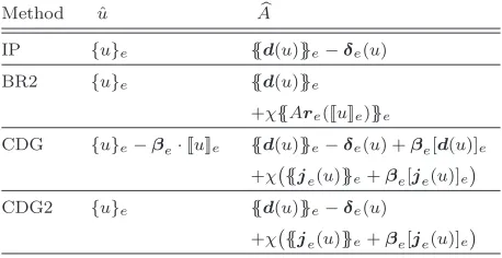
In Table 1 we show the numerical diffusion fluxes ˆu and A considered in this
paper. The numerical fluxes on the boundary are also prescribed in the table based on the definition of the operators [·]e, [[·]]e,{·}e, and{{·}}eon the boundary. The only
exception to this is that ˆu=gD on a boundary intersection.
Remark 1. The term A in the penalty term δe(u) plays an important role in case of a strongly nonlinear system of equations, like in the case of the Navier–Stokes system. The absence of this term leads to insufficient numerical diffusion resulting in suboptimal convergence rates. The stability of the IP method is especially prone
COMPACT AND STABLE DG METHODS A267
Table 1
Numerical diffusion fluxes on an interface e for all methods considered in this paper. For
simplicity we writeuinstead ofuhand use the abbreviationsd(u) =A∇hu,je(u) =ALe(u), and
δe(u) = heη{{A}}e[[u]]ewithη≥0andχ≥0.
Method uˆ A
IP {u}e {{d(u)}}e−δe(u) BR2 {u}e {{d(u)}}e
+χ{{Are([[u]]e)}}e
CDG {u}e−βe·[[u]]e {{d(u)}}e−δe(u) +βe[d(u)]e
+χ{{je(u)}}e+βe[je(u)]e
CDG2 {u}e {{d(u)}}e−δe(u)
+χ{{je(u)}}e+βe[je(u)]e
methods are shown to be completely immune to changes ofη (see section 3). Note
that η is denoted with C11 in other papers, e.g., in [13, 36]. Also note the slight
difference in the definition of the flux for the CDG method compared to [36], where
the method was introduced withχ= 1. Similarly, BR2 was introduced in [4, 5] with
χ = 3 for triangular grids, but we leave the constant χ free, so that we can take
different grid types (triangular, quadrilateral, tetrahedral etc.) into account.
2.2. Convection-diffusion-reaction equations. In this section we briefly dis-cuss a discrete formulation for equations of the form (2.1) based on the diffusion discretization presented in the previous section:
Ω
ϕ∂tuh=BCDR(uh, ϕ) ∀ϕ∈Vh .
(2.9)
The bilinear form is BCDR(uh, ϕ) := −B(u, ϕ) +BCR(u, ϕ) with B given by (2.4),
where this timeuh in (2.4) is time-dependent andAdepends onuh, and
(2.10) BCR(u, ϕ) =
Ω
f(u)· ∇ϕ−
e∈Γ
e
f(u)·[[ϕ]]e+
Ω
ϕs(u) ∀ϕ∈Vh.
The first two summands in (2.10) correspond to the discretization of the convection term and the last summand to the discretization of the reaction term. In the DG context the discretization of the convective terms is well studied, e.g., in [11, 12] and many other papers; possibly a stabilization is required in convection dominated cases as discussed in [15] and references therein. Other stabilization techniques such as entropy viscosity (cf. [25]) or artificial viscosity methods (e.g., [23]) require a diffusion
discretization as presented in the previous section. The convective numerical fluxf(u)
can be any appropriate numerical flux known for standard FV methods, e.g., presented in textbooks [32, 39] on the subject.
3. Theoretical results. In this section we derive coercivity results for the dif-ferent methods for elliptic problems presented in the previous section. The coercivity results are expressed with respect to the grid-dependent norm:
|||v|||2= K∈Th
|v|21,K+ e∈Γ
re([[v]]e)2Ω
forv∈Vh+H1
For the method presented in the previous section the following theorem can be proven. The results for the IP and BR2 methods can be found in the literature, e.g., [2]. The new results are the proofs for the CDG and CDG2 methods.
Theorem 2 (coercivity estimate). Let Th be a conforming grid on Ω such that there is an affine mapping from a fixed reference elementKˆ to each K∈ Th1 and let βe be as in (2.6). Consider the problem (2.2) with A =const and g = 0. For the bilinear form B given in (2.4)the inequality
B(u, u)≥C|||u|||2 ∀u∈Vh
holds for someC >0 if one of the following conditions is fulfilled:
(a) η is chosen sufficiently large and χ≥0 (for IP, CDG, and CDG2),
(b) η≥0 andχ > χ0, where
1. χ0=NTh for the BR2 method,
2. χ0=Nout
Th for the CDG method, and 3. for the CDG2 method
χ0= NTh 4
1 +ν(β),
withν(β) = maxe∈Γi{|Ke−|/|K+
e|}andKe−,Ke+ determined byβ. The mesh-dependent constantsNout
Th andNTh used to defineχ0are given in(2.7)and
(2.8), respectively.
The first part of this theorem is a simple extension of the proof found in [2] and was
also mentioned for the original CDG method, i.e., withχ= 1 in [36]. The generalized
estimate for the coercivity coefficient of the BR2 method is an easy consequence of the discussion in [2, 8]. Therefore, we focus on the results for the CDG and the CDG2 methods. The proof is given in section 3.2.
Before we proceed with the proof of Theorem 2 in section 3.2, we need to summa-rize some properties of the lifting operators that we require for the proof. In the fol-lowing we will use the abbreviationsL(u) = e∈ΓLe(u) andr(u) = e∈Γre([[u]]e).
3.1. Properties of the lifting operators. In the following we assume that the conditions stated in Theorem 2 are satisfied. The following lemmas summarize some simple observations.
Lemma 3. Let β
ebe chosen as in(2.6)ande∈Γi. Then foru∈Vhit holds that
(3.1) suppre([[u]]e) =Ke+∪Ke− and suppLe(u) =Ke− .
Furthermore,Le(u) = 2re([[u]]e) onKe−.
For e ∈ Γ\Γi we have Le(u) = re([[u]]e) for the CDG method and Le(u) = 2re([[u]]e)for theCDG2 method.
COMPACT AND STABLE DG METHODS A269
Proof. The result forrefollows from the definition. For the second part we denote
withτ+
e the restriction of a functionτ ∈Σ onKe+. Similarly τ−e =τ|K−e. Then
Ω
Le(φ)|K+
e ·τ =
Ω
Le(φ)·τe|K+
e =−
e
[[φ]]e· {{τ+e}}e−
e
βe·[[φ]]e[τ+e]e
=−
e [[φ]]e·
1 2τ
+
e +βe·nKe+τ
+ e =− e [[φ]]e·
1 2τ + e − 1 2τ + e
= 0.
(3.2)
Similarly one can show that
ΩL −
e(φ)·τ = 2
Ωr−e([[φ]]e)·τ for anyτ ∈Σ from which the other equality in the lemma follows directly.
Foreon the boundary we have for CDG2 thatβe is defined as in the interior, so
that the result stated above also holds in this case. For the CDG methodβe= 0 and
this gives usLe(u) =re([[u]]e).
The key ingredient in the proof of Theorem 2 is the following lemma, which relates
re(·)|K−e andre(·)|K+e.
Lemma 4. Let Thbe as in the Theorem 2,β
eas in(2.6), ande∈Γi. Then there exists a positive constantαe such that
(3.3) αere([[u]]e)2
Ke− =re([[u]]e)
2
Ke+ ∀u∈Vh.
Moreover, we have αe=|Ke−|/|K+
e|.
If we define for all e∈Γ\Γi αe= 3 (CDG) andαe= 0 (CDG2), we have
(3.4) Le(u)2Ω= 4
1 +αere([[u]]e) 2 Ω
for alle∈Γ.
Proof. In the following we use the abbreviation re = re([[u]]e). Consider the
affine mappingsFe−, Fe+ of the reference element ˆK toKe−, Ke+, respectively, such
that Fe−1+(e) = Fe−1−(e) and with an orientation such that for all i ∈ 1, N (N =
dim Σh(Ke−) = dim Σh(K+
e))
ˆ
τi◦Fe−1+(x) = ˆτi◦Fe−1−(x) ∀x∈e,
for some orthonormal basis{τˆi}i=1,N of Σh( ˆK). Consequently,{τ±i = ˆτi◦Fe−1±}i=1,N
is an orthogonal basis of Σh(Ke±) such thatτ−i =τ+i =:τe,i one. By settingτ±i to
zero outside ofK± we obtain functions in Σh. Let us introduce the notation
r±
e =
re onKe±,
0 elsewhere.
We can now representr−e,r+e onKe± in the basis{τi±}, i.e.,r±e = iN=1r±e,iτ±i , and we introduce
be=− 1 2
e
[[u]]e·τe,i
i=1,N
, r±e =re,i±
i=1,N, M
±
e =
K±e
τ±
i ·τ±j
i,j=1,N
.
By definition of the lifting operators (2.5) we compute
(3.5)
Ke±
r±
e ·τ±i =
Ω
re·τ±i =−
e
[[u]]e· {{τ±i }}e=−1 2
e
Consequently, we have
r±e = (Me±)−1 be.
Since
K±(r±e)2=r±e ·Me±r±e we conclude that
re2K±
e = (M
±
e )−1 be·be= 1
|Ke±||be| 2.
For the last equality we used the fact that we are working with an orthonormal set of
basis functions so that the mass matrix satisfiesMe±=|K±|I, whereI is the identity
matrix inRN×N. Thus we can choose αe = |Ke−|
|Ke+| in (3.3). To show (3.4) we notice
first that re2
K−e = (1 +αe)
−1r
e2Ω, sincere2Ω =re2K−
e +re
2
Ke+. Now, it is easy to see from Lemma 3 that (3.4) is fulfilled.
Note that although we used an orthonormal basis function in the proof of Lemma 4, the coercivity result does not depend on this choice. Also note that the assumption of Lemma 4 requires that the grid is conforming and that each grid element is an affine mapping of a same reference element. These grids include, for example, simplicial grids, Cartesian grids, or a grid whose elements are parallelograms in two dimensions, or parallelepipeds in three dimensions.
Finally, our analysis requires the following estimate on the lifting operator re,
with a proof in [8].
Lemma 5 (see Brezzi et al. [8]). There is a positive constant C2 independent of
heandusuch that
re([[u]]e)2Ω≤C2h−1e [[u]]e2e for eachu∈Vh and for each e∈Γ.
3.2. Proof of Theorem 2 for the CDG and CDG2 methods. To carry out
the proof of Theorem 2 we first rewrite the bilinear form using parameters β1, Le,
andδe and assumingA≡1:
B(uh, ϕ) =
Ω
∇uh· ∇ϕ+χ
e∈Γ
Ω
Le(ϕ)·Le(uh)
+
e∈Γ
e
({{∇ϕ}}e·[[uh]]e+{{∇uh}}e·[[ϕ]]e)
+β1
e∈Γi
e
βe·
[∇uh]e[[ϕ]]e+ [∇ϕ]e[[uh]]e
−
e∈Γ
e
δe(uh)·[[ϕ]]e ∀ϕ∈Vh. (3.6)
We haveβ1= 1 for CDG, andβ1= 0 for all other methods,Le is zero for IP, equal
to Le for CDG, CDG2, andLe(·) = re([[·]]e) for BR2, and finally δe =δe for IP,
CDG, CDG2 and zero for BR2.
First we prove the coercivity result for the CDG method.
Proof(for the CDG method). We note that the bilinear form of the CDG method can be written in the following form:
(3.7) B(u, u) =∇u+L(u)2Ω− L(u)2Ω+χ
e∈Γ
Le(u)2Ω+
e∈Γ
η
he[[uh]]e 2
COMPACT AND STABLE DG METHODS A271
SinceLe= 0 on allKwhere eis an inflow edge, we have
(3.8) L(u)2Ω≤NTout
h
e∈Γ
Le(u)2Ω.
For anyε∈(0,1) we obtain
∇u+L(u)2Ω≥ K∈Th
(1−ε)|u|21,K+ (1−ε−1)L(u)2Ω,
which follows from the Cauchy–Schwarz inequality. Furthermore, from Lemma 5, inequality (3.8), equality (3.4), and the last inequality we get
B(u, u)≥ K∈Th
(1−ε)|u|21,K+ e∈Γ
4
1 +αe(χ−ε −1Nout
Th ) +ηC2−1
re2Ω.
If condition (a) of Theorem 2 is satisfied we can choose η large enough that the
coefficient of the second sum becomes positive. If condition (b) is satisfied, we can
chooseε so close to 1 that χ−ε−1Nout
Th becomes positive. The positive number C
from the formulation of the theorem is now the minimal value of the positive numbers 1−εand 1+4α
e(χ−ε
−1Nout
Th ) +ηC
−1 2
We now continue with the proof for the CDG2 method.
Proof(for the CDG2method). In the case of the CDG2 method the bilinear form
B(u, u) can be rewritten as
B(u, u) =∇u+r(u)2Ω− r(u)2Ω+χ
e∈Γ
Le(u)2Ω+
e∈Γ
η he[[u]]e
2
e.
Note that re(·) ≡ 0 in grid elements not having e as one edge. From that fact we
derive the inequality
(3.9) r(u)2Ω≤NTh
e∈Γ
re([[u]]e)2Ω.
As in the proof for the CDG method we get
∇u+r(u)2Ω≥ K∈Th
(1−ε)|u|21,K+ (1−ε−1)r(u)2Ω
for anyε∈(0,1). Combining Lemma 5, inequality (3.9), and the last inequality we
obtain
B(u, u)≥ K∈Th
(1−ε)|u|21,K+ e∈Γ
4χ
1 +αe −ε
−1N
Th+ηC2−1
re2Ω.
Note thatαe= 0 fore∈Γ\Γi. By similar arguments as in the CDG case, we conclude
that we can chooseηlarge enough if condition (a) of Theorem 2 is satisfied, orεclose
to 1 if condition (b) is satisfied, so that both coefficients in front of|u|1,Kandre2
Ω
are positive. The positive numberC from the formulation of the theorem is now the
minimal value of the positive numbers 1−εand 4χ
1+αe−ε
−1N
3.3. Further remarks. Following the discussion from [2] one can prove for bounded, coercive, consistent, and adjoint consistent methods the following a priori
error estimate for the discrete solution of a linear elliptic problemuh∈Vh:
(3.10) u−uhΩ≤Chk+1|u|k+1,Ω
if the exact solutionuis inHk+1(Ω)∩H1
0(Ω). HereCis a constant andkis the
poly-nomial degree of the basis functions fromVh. All the methods studied in this paper
fall into this category. It is straightforward to see that all the methods studied here are consistent and adjoint consistent; Theorem 2 gives conditions for their coercivity, and boundedness can be shown using the estimates found in [2].
From the coercivity results one can conclude theL2-stabilityestimate d
dt
Ωu2≤0
in the parabolic case for each method. The stability proof for the case that both convection and diffusion terms are present can be treated as described, for example,
in [13] under suitable conditions on the numerical fluxf. The arguments found there
demonstrate that it suffices to concentrate on the diffusion part.
In the case of the CDG2 method the switch function can be chosen such that
χ0= NTh
2 , independent of the underlying grid as we will show in the following section.
This observation turns out to be crucial, because choosing the smallest lifting and stability factor which guarantee stability leads to the most efficient method.
We conclude this section with the observation that on some special meshes, i.e., Cartesian meshes as well as triangular meshes created out of Cartesian meshes by dividing each quadrilateral into two triangles, the BR2 and CDG2 methods coincide when applied to linear problems.
Corollary 6 (BR2 and CDG2 on special meshes). Consider the setting of Theorem 2. The methodsBR2andCDG2coincide on grids Thwith|K1|=|K2|and equal shape for allK1, K2∈ Th if χBR2= 2χCDG2 andδe(u)≡0.
Proof. This result is a consequence of observing that in this situationΩLe(u)·
Le(ϕ) = 4
Ke−re([[u]]e)·re([[ϕ]]e) and
Ωre([[u]]e)·re([[ϕ]]e) = 2
Ke−re([[u]]e)·re([[ϕ]]e)
holds. The last equality follows from
K+e re([[u]]e)·re([[ϕ]]e) =
Ke−re([[u]]e)·re([[ϕ]]e)
as can be shown using change of variables since there exists an affine mappingF of
K+
e into Ke− such that re([[u]]e)(x) = re([[u]]e)(F(x)),re([[ϕ]]e)(x) =re([[ϕ]]e)(F(x)), and |det(D(F(x))/Dx)|= 1 for all x ∈ K+
e. Thus for the two methods the term
ΩLe(ϕ)·Le(uh) in (3.6) differs only by a factor of 2.
4. Implementation. In this section we provide some details on our implemen-tation of the compact DG methods presented in this paper, focusing once again on
the CDG and CDG2 methods. Our implementation is part of the Dune-Fem
mod-ule [16], which is based on the free software environmentDune [6, 7]. Dune-Fem
provides a range of different methods for solving general systems of nonlinear partial differential equations on parallel, locally adapted grids.
Employing the DG method for the spatial discretization of a convection-diffusion-reaction equation leads to
Ω
ϕ∂tuh=BCDR(uh, ϕ) ∀ϕ∈Vh
(4.1)
for the semi-discrete function uh with uh(t,·) ∈ Vh. The bilinear form BCDR is
described in section 2.2. Writing uh(t, x) = iui(t)ϕi(x), where{ϕi}i forms a basis
ofVh, we arrive at a system of ODEs
COMPACT AND STABLE DG METHODS A273
and M is the mass matrix
Ωϕiϕj
i,j. Thus solving the system of evolution
equa-tions requires computing the bilinear formBCDR(uh(t,·), ϕi), the inverse of the mass matrix, and solving the resulting system of ODEs.
4.1. Spatial discretization. In the Dune-Fem framework either Lagrange type basis functions or orthonormal basis functions are available to build the discrete
space Vh. For the work presented here we have used an orthonormal basis, so that
the mass matrix is diagonal. All our numerical experiments have shown that taking
η= 0 in the CDG and CDG2 methods leads to the best results ifχis taken according
to Theorem 2 part (b). Therefore we will only present details of the implementation
for the schemes withη= 0.
Assuming now that the test functionϕ=ϕi has support on only one elementK
of the gridThand denoting withuK the restriction ofuhtoK,B given in (2.4) takes
on a much simpler form. We use the definition of the jump and average operators and the unified formulation of the fluxes found at the beginning of section 3.2 to arrive at
BCDR(uh, ϕ) =−
K
(f(uK)· ∇ϕ+sE(uK)ϕ) +
e⊂∂K
f(u)·neϕ
+
K
(A(uK)∇uK· ∇ϕ−sI(uK)ϕ)−
e⊂∂K
A(u)·neϕ
−
e⊂∂K∩Γi
1
2+β1βe·ne
A(uK)[[u]]e· ∇ϕ
−
e⊂∂K∩∂Ω
(uK−gD)A(uK)ne· ∇ϕ
=:BE(uh, ϕ) +BI(uh, ϕ),
(4.2)
with β1 = 1 for CDG and 0 for all other methods. InBE we combine the first two
integrals which discretize the convection forces and a part of the source term sE.
The second termBI contains the diffusion and the remaining part of the source term
denoted with sI =s−sE. This splitting is used to employ a semi-implicit (IMEX)
ODE solver as described later in this section.
It remains to study the implementation of the convective fluxfand the fluxAfor
the diffusion in the primal formulation (2.4). For the convection we use theRusanov
fluxdescribed, for example, in [39]. Using (3.2) we obtain the following representation
for the diffusion fluxA(u):
(4.3) A(u) =
⎧ ⎪ ⎨ ⎪ ⎩
{{A(u)∇u+χA(u)re([[u]]e)}}e BR2,
A(u)∇u+ 2χA(u)re([[u]]e)|K−
e CDG,
{{A(u)∇u}}e+ 2χA(u)re([[u]]e)|K−
e CDG2.
Hence we see that for the BR2 method, as well as for the CDG, CDG2 methods, we
need only compute the liftingre. While for the BR2 methodremust be computed on
both elementsKe−, K+
e, for the CDG and CDG2 we have to compute the lifting only
onKe−depending on the switch functionβe. To computereonKe−or onK+
e we can
make use of the fact that we are using orthonormal basis functions. Thus the degrees of freedom (ri)idefiningre([[u]]e) onKare easily computed throughri=−12e[[u]]e·τi,
where (τi)i is an orthonormal basis ofPk(K)d. The lifting required for the CDG and
CDG2 methods therefore involves only the computation of a single integral over each
intersection e ∈ Γi and can be computed while the fluxAover that intersection is
It remains to fix the switch βe for each interior edge e ∈ Γi. One suggestion,
which is widely used in the literature [13, 2, 36], is theupwind switch
(4.4) βe= 1
2sgn(nKe·w)nKe .
The upwind vector w ∈ Rd is chosen a priori (i.e., before each time step), so that
w·n = 0 for the normal n to ∂K for all K ∈ Th. Thus Ke− is chosen to be the
element adjacent toewithnK−
e ·w>0.
Our suggestion is motivated by the coercivity estimate for the CDG2 method.
According to Theorem 2, the CDG2 method is stable providedχ > NTh
4
1 +ν(β).
The efficiency of the method is severely influenced by the magnitude of χ, larger
values increasing the condition number of the system matrix. Thus it is advantageous to renderν(β) = maxe∈Γi{|Ke−|/|K+
e|}as small as possible. This can be achieved by
using thearea switch
(4.5) βe= 1
2nK∗e ,
whereKe∗ is the element adjacent toewith the smaller area. Thus|Ke−| ≤ |K+
e|and
consequentlyν(β)≤1.
4.2. Temporal discretization. Using the splitting defined in (4.2) together with the method of lines described above leads to a system of ODEs
(4.6) U(t) =FE(U(t), t) +FI(U(t), t),
where U(t) = (ui(t))i is the vector of degrees of freedom for the unknown function
uh(t, x) = iui(t)ϕi(x) and the components of FE andFI are M−1BE(uh(t,·), ϕi) and M−1BI(uh(t,·), ϕi), respectively. To avoid the strong time step restriction
im-posed by the diffusion and stiff sources (combined intosI), we want to use an implicit
method for these terms, while allowing for time exact simulation of the convection forces, through an explicit treatment of these terms.
For the numerical examples we use IMEX Runge–Kutta methods of orderk+ 1,
where k is the polynomial order of the basis functions used to construct Vh. For
k= 1 we use the IMEX-SSP2(2,2,2); details on the corresponding Butcher array can
be found in [35]. A detailed convergence analysis for the IMEX-SSP2(2,2,2) and a
DG method for convection-diffusion equations is carried out in [9]. Fork= 2 we use
the method YZ(3,3) presented in [40], and fork= 3 we use the IERK(4,5) presented
in [33].
Using these methods the time step ΔtEis merely restricted by the CFL condition.
Note that fully implicit methods could also be used, in which case the bilinear form is not split into two parts.
Implicit methods naturally lead to large systems of nonlinear equations, increasing in size if higher order Runge–Kutta methods are used. In our implementation we reduce the size by using diagonally implicit methods, but nevertheless the resulting nonlinear algebraic system is large and difficult to solve. To avoid the computation of
the Jacobian of the function FI we use a matrix free Newton solver. Since our time
COMPACT AND STABLE DG METHODS A275
In each step of the Newton iteration a linear system of the formDFn
I δn=−FIn,
whereFn
I =FI(Un, t) required the evaluation of the bilinear formBI. This linear
sys-tem is solved using a CG type method (BiCG-stab or GMRES for nonsymmetricA).
Instead of using the exact Jacobian we use a one sided approximation toDFn
I . Since
the iterative solvers used require only the implementation of the application of the
linear operatorDFIn to given vectorsv1, . . . , vS, we can use the following
approxima-tion DFInvs = ε1n(FI(Un+εnvs)−FIn). Thus only one application of the bilinear
form is required in each iteration steps= 1, . . . , S of the linear solver. The step size
εn is computed following the suggestions found in [31]: ε=ε
dbl1+|U
n|
|v|2 .
4.3. Choice of parameters in the CDG and CDG2 methods. In contrast to the IP method, CDG is quite robust with respect to the choice of the penalty
parameterη. As was already pointed out in [36], the original CDG method (taking
χ = 1) is very stable even with η = 0 at least on 2D triangular grids. In this case,
we have not been able to construct examples where the system matrix has negative eigenvalues, at least in the case of the Laplace operator. Only when used to discretize
the operator−∇·A(x)∇u(x), we found problems with stability in some cases, which
could be solved by a slight increase of eitherηorχ. A second case, where we observed
negative eigenvalues even for the Laplace operator when taking the CDG method in its original formulation, was on some quadrilateral grids.
The three-dimensional (3D) setting was not tested in [36] and here we did en-counter problems even for the Laplace equation when using the CDG method with
χ= 1. For Test Case 1 of the 3D Benchmark on Discretization Schemes for Anisotropic
Diffusion Problems on General Grids (cf. [21]) using meshtet.0.msh, we discovered
that with χ= 1 the minimal eigenvalue of the stiffness matrix was−12.167 so that
the bilinear form B is not coercive in this case. This example demonstrates the
ne-cessity of using a constantχ >1. In numerical experiments we discovered thatχcan
be chosen smaller than the bounds given in Theorem 2. However, these values differ from method to method, from problem to problem, and from grid to grid. For those
reasons we choose for the CDG, CDG2, and BR2 methods χ =χ0 in all numerical
experiments presented in section 5.
For our comparison with the much simpler IP method, we choose the parameter
η on eache∈Γ as suggested in [1]:
(4.7) ηe=1
2 Kmax∈Th e∈∂K
k(k+ 1)λAmax
e∈∂K
Λe|e|2
|e|2 ∀e∈Γ.
Here k is the polynomial order of the basis functions andλA
max denotes the largest
eigenvalue of the diffusion matrix A. Λe = 1/2 if e∈Γi, Λe = 1 if e is part of the
Dirichlet boundary, and Λe = 0 for Neumann boundaries. In [1] it is shown that
choosing ηe
he in the stability term with hedefined in section 2.1 results in coercivity
for the IP method on triangular grids in two space dimensions. Alternative choices of
the parameterηeare, for example, given in [19, 20].
Navier–Stokes system. Further models for which we have employed these methods include flow problems with detailed chemical reaction and free surface shallow water flow.
We focus on a comparison of the efficiency of the methods, i.e., we compare their
error to runtime ratio. In all numerical examples we choose the parametersη andχ
according to the theoretical bound given by Theorem 2. For the CDG, CDG2, and
BR2 methods this means thatη= 0 and stability is achieved by choosingχ equal to
the boundχ0 given by Theorem 2. For the IP method the penalization coefficientη
is chosen according to (4.7).
(a) mesh1 (b) structured mesh (c) unstructured mesh
Fig. 1. Two structured and one unstructured macrotriangulation.
5.1. Elliptic problem. In the first example we consider a linear elliptic problem of the form
−∇ ·(A∇u) = 0 in Ω = [0,1]2, u=g on∂Ω, A=
1 0
0 ε
.
(5.1)
If the boundary conditions are defined byg(x, y) = sin(2πx)e−2π
√
1/εy, then u≡g
is a solution to this problem. For the following numerical experiment we choose
ε = 103. This problem corresponds to Test 2 of the Benchmark on Anisotropic
Diffusion Problems presented at the FVCA 5 [28]. Note that for the CDG scheme
results for all test cases of the benchmark can be found in [14]. For the current 3D
Benchmark on Anisotropic Diffusion Problems results for the CDG2 method can be found in [30].
The calculations are performed on mesh1of the benchmark, presented in
Fig-ure 1(a). For the EOC calculation this mesh is refined by quartering all elements in each step. The tolerance for the linear solver has been chosen sufficiently small to obtain optimal convergence rates. The parameters for the DG methods are (according
to Theorem 2) BR2χ= 3, CDGχ= 2, and CDG2χ= 1.5. For the IP method the
stability coefficient has been chosen as described in (4.7). For the CDG method we
used theupwind switch and for the CDG2 method thearea switch.
All methods considered show the expected convergence rate ofk+ 1,kbeing the
polynomial order of the basis functions used to build Vh. Differences in terms of L2
-accuracy between BR2, CDG, and CDG2 on a fixed grid are usually lower than 5%,
but for the IP method we get up to 25% higherL2-errors. In Figure 2 we compare
L2-error and computational time required for solving the linear system. We see that
COMPACT AND STABLE DG METHODS A277
Fig. 2.CPU time toL2-error comparison for the elliptic problem(5.1). Left, the CPU time for
the CG solver. Right, CPU time for the CG solver andILU(0) preconditioning is plotted. Solver
and preconditioner from PETSc[3]have been used.
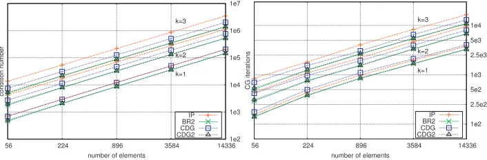
Fig. 3.Condition number (left), calculated with the Krylov–Shur method implemented in SLEPc
[29], and iterations of the CG solver (right) for the Poisson equation on a triangular grid for
k= 1,2,3.
solver makes sense in our setting since we want to apply the methods in a matrix free solver where the application of preconditioning is very difficult.
In Figure 3 we present the condition number which is λmax/λmin where λmax
is the largest eigenvalue of the bilinear form B and λmin the smallest eigenvalue.
[image:16.612.80.435.91.213.2]The eigenvalues have been calculated using the Krylov–Shur method implemented in the software package SLEPc [29]. As we can see, CDG2 and BR2 have the smallest condition number followed by CDG, while IP has the largest condition number. In this example a smaller condition number coincides with fewer iterations of the linear solver needed to achieve a certain reduction of the error, plotted in the right part of Figure 3. We can see that for this example the CDG2 and the BR2 methods seem to be the best choice since they are the most accurate and efficient. In a matrix free implementation, CDG2 could be expected to have a slight advantage over BR2 since the evaluation of the bilinear form is more expensive for the BR2 method, where the
lifting operatorrehas to be evaluated twice as much as for the CDG2 method. The
approximation quality and the efficiency of the IP method are inferior to those of BR2, CDG, and CDG2 in our example. Additionally, although for the IP method
no lifting operator has to be evaluated, the calculation of the parameterηe in (4.7)
depends on the largest eigenvalue of the diffusion matrix A. These computations of
eigenvalues can become very difficult for nonconstant A or for nonlinear systems of
[image:16.612.73.426.270.386.2]upper bound for the eigenvalue leads to an over excessive penalization, increasing the condition number of the system matrix and thus the efficiency of the scheme.
5.2. Linear parabolic problem. In the second example we consider a 2D linear advection-diffusion equation of the form
∂tu+∇ ·(uv)−εΔu= 0 on [0,1]2×[0, tend], u(·,0) =u0 on [0,1]2,
(5.2)
for which we can construct an exact analytical solution which we use to prescribe the
Dirichlet boundary data. We take a constant velocityv = (0.1,0.2) andε= 0.1. The
initial data is given byu0(x, y) = Nn=1un0(x, y) withun0(x, y) = (αx,ncos(γx,nπx) +
βx,nsin(γx,nπx))(αy,ncos(γy,nπy) +βy,nsin(γy,nπy)) withN= 2 andαx= (0.6,0.9),
αy= (1.2,0.3),βx= (0.8,0.2), βy = (0.4,0.1), andγx= (2,0.7), γy= (1,0.5). With this choice we have
u(t, x, y) = N
n=1
e−πεt(γx,n+γy,n)un
0(x, y).
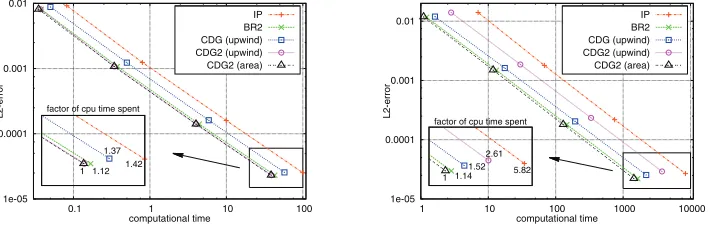
In Figure 4 we compare the efficiency of the different schemes by studying runtimes
and discretization errors attend= 0.1 in theL2norm. For this problem we show only
results for k = 2 but use two different grids. The first grid is a regular criss-cross
grid (see Figure 1(b)) obtained refining a macrogrid consisting of a Cartesian grid where each cube element is split into two triangles. Thus each element of the grid has the same volume so that CDG2 and BR2 are identical in this case (see Corollary 6). This can be seen in the results since on a fixed refinement level, both CDG2 and BR2 lead to the same error. In this case the CDG2 method is more than 10% more
efficient, due to the lower cost in evaluating the bilinear form B. IP is the least
efficient scheme, followed by CDG. The second grid is a highly unstructured grid (see
Figure 1(c)). Due to the larger value ofν(β), the CDG2 method with the upwind
switch is considerably less efficient than BR2 and in this case even less efficient than
CDG. Using the area switch leads to ν(β) ≤ 1 and the method is again the most
efficient one, outperforming BR2 again by more than 10%.
1e-05 0.0001 0.001 0.01
0.1 1 10 100
L2-error
computational time IP BR2 CDG (upwind) CDG2 (upwind) CDG2 (area)
factor of cpu time spent
1 1.12 1.37
1.42
1e-05 0.0001 0.001 0.01
1 10 100 1000 10000
L2-error
computational time IP BR2 CDG (upwind) CDG2 (upwind) CDG2 (area)
factor of cpu time spent
1 1.14 1.52
2.61
5.82
Fig. 4.Results for the advection-diffusion problem. TheL2-error on a triangular grid fork= 2
is plotted with respect to the runtime. On the left, a criss-cross grid is used, leading to theoretical
parameters of χ= 2 (CDG), χ= 3 (BR2), andχ= 1.5 (CDG2). On the right, results on the
unstructured grid are shown; the theoretical parameters for this setting are the same for all methods
except for the CDG2method with upwind switch where we haveχ= 8.4375. For the IP method the
[image:17.612.83.438.509.622.2]COMPACT AND STABLE DG METHODS A279
5.3. Nonlinear parabolic problem. As a third example we consider the time-dependent compressible nonlinear Navier–Stokes equations
∂tu+∇ ·(F(u)−A(u)∇u) =s(u) in Ω×[0, tend],
(5.3)
whereu= (ρ, ρv, ρe),ρis density,ρv momentum vector, andρetotal energy. In this
section we will restrict ourselves to two dimensions for the sake of simpler notation. The convective and diffusive fluxes are given as
F(u) = ⎡ ⎢ ⎢ ⎣
ρu ρw
ρu2+p ρuw ρuw ρw2+p u(ρe+p) w(ρe+p)
⎤ ⎥ ⎥
⎦, A(u)∇u= ⎡ ⎢ ⎢ ⎣
0 0
τ11 τ12 τ21 τ22 Ediff1 +κ∂xT E2diff+κ∂zT
⎤ ⎥ ⎥ ⎦
with E1diff =uτ11+wτ21 and E2diff = uτ12+wτ22. The viscous stress tensor τ for
Newtonian fluids is defined as
(5.4) τ =
(2μ+λ)∂xu+λ∂zw μ(∂xw+∂zu)
μ(∂xw+∂zu) λ∂xu+ (2μ+λ)∂zw
;
κis thermal conductivity coefficient. The termκ∇Trepresents the heat flux according
to the Fourier’s law. In the convective and diffusive fluxes we have other unknowns
pand T, which are related touby
(5.5) p= (γ−1)ρ
e−1
2v
2
, T =p/(ρRd),
whereRd=cp−cvis the specific gas constant of the dry air andγ=cp/cvis the ratio
of specific heat capacity at constant pressurecp and at constant volumecv. Finally,
we close the system of equations with λ =−23μ and κ=cpμPr−1, where Pr is the
Prandl number.
For this test case we choose parameters and exact solution similar to [24]:
ρ=e= 1
2sin(π(x+y)−t) + 2 and v= (1,1),
withμ= 0.1, Pr = 0.72,cp= 1004, andcv= 717. The source termsin (5.3) is chosen
so that we have an analytical solution. The computational domain is Ω = [0,2]2.
In Figure 5 we compare CDG2 with area switch with CDG and BR2 at the
end-timetend= 0.1. We use the same time integration scheme for all methods of the same
order. These time integrators have been described in section 4.2. On the left picture of Figure 5 we observe that the CDG2 method of order 2, 3, and 4 is at least 10% faster in terms of the CPU time than BR2 of the corresponding order, and more than
35% than CDG, whereas the difference in theL2-error is less than 4% for all methods.
We also observe that the GMRES solver, in case of the CDG method, needs 54% more iterations for the whole simulation than in the case of CDG2 and BR2, which require the same number of iterations.
1e-5 1e-4 1e-3 1e-2 1e-1 1e+0
1e-1 1e-0 1e+1 1e+2 1e+3 1e+4
L2-error
computation time k=1
k=2
k=3 BR2 CDG CDG2
1 1.12 1.58 factor of cpu time spent
1e+3 1e+4 1e+5 1e+6
96 384 1536 6144
GMRES iterations
grid elements
BR2 CDG CDG2
Fig. 5.Results for Navier–Stokes equations on an unstructured triangular grid. The
stabiliza-tion parameters areη= 0andχaccording to Theorem2.
1e-06 1e-05
10 100 1000
L
2-error
computation time CDG2 (A)
BR2 (A) CDG2 (B) BR2 (B)
A
Scheme CPU time L2-error
CDG2 305 3.91e-07
BR2 329 3.92e-07
B
Scheme CPU time L2-error
CDG2 1790 5.47e-07
BR2 2469 5.46e-07
Fig. 6. Comparison on affine (A) and nonaffine (B) quadrilateral grids. Problem is
from section 5.2 on the quadrilateral domain with corners (0,0),(1,0),(1,1),(0,1) (A) and
(0.4,0),(1,0),(1,1.4),(0.1) (B). The graph (left) contains levels 4 and 5 of the simulation cycle
and the table (right) contains the numbers of the level5run.
for linear problems. Furthermore, we show that these conditions can be successfully used for nonlinear Navier–Stokes equations. Numerical examples for Poisson, linear heat, and nonlinear Navier–Stokes equations show that CDG2 is more efficient than
CDG in terms ofL2-error versus CPU time. On very regular grids the CDG2 method
is identical to the BR2 method whereas the spatial operator of the CDG2 is slightly cheaper to evaluate.
Our results indicate that even on triangular grids using orthonormal basis func-tions the CDG2 method is more efficient than BR2, even though in this case the lifting operator is cheap to evaluate. In Figure 6 we show results on two quadrilateral grids, the second one requiring nonaffine element transformations. We use a natural
extension of the bounds in Theorem 2 to define χ. Note that in this situation the
mass matrix is no longer diagonal and the lower complexity of the CDG2 method in this case clearly leads to a more efficient method. Due to the still missing theoreti-cal justification of bounds for the parameter values this situation still requires more thorough testing.
Acknowledgments. The authors would like to thank the reviewers and the editor for their various important remarks and suggestions. Computations have been
[image:19.612.76.435.99.220.2] [image:19.612.77.410.270.387.2]