Study of the best linear approximation of nonlinear systems with arbitrary inputs

(1)

University of Warwick institutional repository: http://go.warwick.ac.uk/wrap

A Thesis Submitted for the Degree of PhD at the University of Warwick

http://go.warwick.ac.uk/wrap/57859

This thesis is made available online and is protected by original copyright.

Please scroll down to view the document itself.

(2)

Study of the Best Linear Approximation

of Nonlinear Systems with Arbitrary Inputs

by

黃顯鈞

Wong, Hin Kwan Roland

Thesis

Co-tutelle of

University of Warwick, U.K. & Vrije Universiteit Brussel, Belgium

for the degree of

Doctor of Philosophy

School of Engineering,

University of Warwick

Faculty of Engineering,

Vrije Universiteit Brussel

(3)

Supervisors

Prof. Nigel G. Stocks

University of Warwick, U.K.

Prof. em. Keith R. Godfrey University of Warwick, U.K.

Prof. Johan Schoukens

Vrije Universiteit Brussel, Belgium

Members of the Jury

Prof. Steve Vanlanduit (President) Vrije Universiteit Brussel, Belgium

Prof. Johan Deconinck (Vice President) Vrije Universiteit Brussel, Belgium

Prof. Gerd Vandersteen (Secretary) Vrije Universiteit Brussel, Belgium

Prof. Jérôme Antoni

Université de Lyon, France

Prof. Tadeusz P. Dobrowiecki

Budapest University of Technology and Economics, Hungary

Dr. Ai Hui Tan

Multimedia University, Malaysia

Prof. Peter R. Jones

University of Warwick, U.K.

(4)

List of Figures

1.1 TheBlas of a static pure cubic nonlinearity identiﬁed by three types of input signals . . . 6

2.1 Dft power spectrum of a typical periodic Dirbs of period 𝑁 = 511

with levels±1 . . . 16

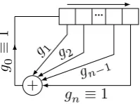
2.2 Fibonacci implementation of Lfsr . . . 19

2.3 Illustrating and the generation of an Mlbs of period𝑁 = 7 using a 3-bitLfsr . . . 20

2.4 Dftpower spectrum of a typicalMlbsof period𝑁 = 511with levels

±1 . . . 22

2.5 Periodic autocorrelation function of aZoh Mlbswith bit-interval of

𝑇, period𝑁𝑇and levels ±1 . . . 22

2.6 Dft power spectrum of a typicalIrbs of period𝑁 = 510 with levels

±1 . . . 25

3.1 Wiener-Hammerstein system structure . . . 33

3.2 Wiener system structure . . . 35

3.3 Comparison of simulation against theory: Blas (with dc gain norm-alised) obtained from Gaussian and binary inputs plotted with their theoretical counterparts for a Wiener system with pure cubic non-linearity . . . 40

3.4 Comparison of simulation against theory: Blas (with dc gain norm-alised) obtained from Gaussian and binary inputs plotted with their theoretical counterparts for a Wiener system with pure quintic non-linearity . . . 42

3.5 Generic Volterra system structure. . . 44

(10)

3.6 Empirical (measured) Discrepancy Factors obtained from random binary sequences and Gaussian noise againsttheoretical Discrepancy Factors for various Wiener systems with pure cubic nonlinearity (sim-ulation) . . . 50

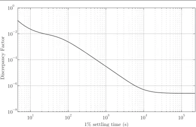
3.7 Discrepancy factor as a function of settling time of a ﬁrst order lin-earity in a Wiener system . . . 51

3.8 z-plane plot of the various poles conﬁgurations of the second order linearity used in Section 3.5.2 . . . 52

3.9 Discrepancy factor as a function of the settling time of a second order linearity in a Wiener system . . . 53

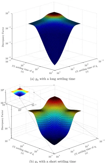
3.10 Discrepancy Factor of a cubic nonlinearity 3-branch parallel Wiener system with linearities of various settling time . . . 54

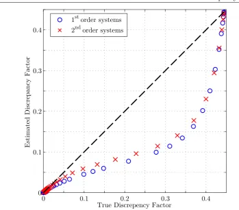
3.11 The estimated and true Discrepancy factors in various Wiener ﬁrst and second order systems . . . 55

4.1 The robust procedure for estimating the BLA . . . 59

4.2 Power spectrum of a typical Dirbs of period 𝑁 = 500 with thicker circles indicating frequencies with near zero power . . . 61

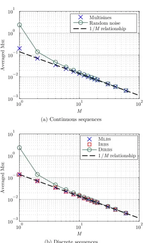
4.3 Performance comparison of various stochastic and invariant spectrum sequences against number of realisations of input . . . 64

4.4 Discrete Wiener system block diagram with noisy output (Oemodel) 65

4.5 Performance comparison between Irbs, Mlbs and Dirbs as inputs to a Wiener system with even and odd order nonlinear distortions . 67

4.6 Performance comparison between Irbs, Mlbs and Dirbs as inputs to a Wiener system with only odd order nonlinear distortions . . . . 67

4.7 Illustration of the diﬀerence in behaviour of nonlinear distortions . . 70

4.8 Rse of the median and the mean against sample sizes in estimating Gaussian population mean. . . 76

4.9 Log scale box-plot of absolute estimation errors of a section of a best linear impulse response 𝑔[𝑟]̂ for 𝑟 between 30 and 80 using 𝑀 = 10

diﬀerent M-sequences without output noise disturbances.. . . 79

4.10 Estimation error of the Best Linear Approximation (Bla) from output-noise-free measurements against number of Mlbs input realisations (𝑀) used in averaging when using either mean or median averaging schemes. . . 80

4.11 Identiﬁcation performance of various averaging schemes against Snr

levels . . . 81

(11)

5.1 Designing the p.m.f. of a discrete symmetric ternary sequence . . . . 88

5.2 The p.m.f. of a symmetric ternary sequence tuned for Gaussianity . 88 5.3 Designing the p.m.f. of a discrete symmetric quaternary sequence . . 89

5.4 The p.m.f. of a symmetric quaternary sequence tuned for Gaussianity 89 5.5 Designing the p.m.f. of a discrete symmetric quinary sequence . . . . 90

5.6 The p.m.f. of a symmetric quinary sequence tuned for Gaussianity . 90 5.7 Discrepancy Factors of random ternary sequences with various zero-level probabilities . . . 93

5.8 Illustration of the diﬀerence between Bla’s estimated from various multilevel uniform and optimised sequences . . . 94

6.1 System schematic for the physical experiment setup in Chapter 6 . . 98

6.2 Equivalent system structure of Fig. 6.1 . . . 99

6.3 The use of supersampling and subsampling . . . 102

6.4 Identiﬁcation of the RC Linearity with op-amp based pre- and post-buﬀers, case 1 . . . 105

6.5 Experiment result of the identiﬁcation of theBlawith Gaussian and binary inputs for an electronic Wiener system with non-ideal cubic nonlinearity and a RC linearity, case 1 . . . 107

7.1 Wiener-Hammerstein system structure . . . 112

7.2 Bode plot comparing the high frequency ﬁtting of 𝐺_Bla_{, A} and 𝐺_Bla_{, B} 115 7.3 Rms errors from running optimisation (up to degree 8) on all realis-able zero-pole allocations in a Wiener-Hammerstein structure. . . 118

7.4 Graphs of nonlinearity output 𝑤versus input𝑥 . . . 119

7.5 Comparison between the gain responses of the estimated transfer functions 𝐺₁ and 𝐺₂ with theoretical values.. . . 124

7.7 Eﬀect of polynomial degree on simulation error . . . 128

7.8 Eﬀect of dual-polynomial degree on simulation error . . . 128

7.9 Model output and simulation error for the training data set . . . 129

7.10 Dftspectra of the model output (black) and simulation error (grey) for the training data set . . . 130

(12)

7.11 Static nonlinearity characteristic using coeﬃcients from ﬁlter ID 30 . 131

8.1 Overview of the Peltier cooling system . . . 137

8.2 Block diagrams of Subsystems 1and 2 . . . 137

8.3 Overview of the Peltier cooling system . . . 139

8.4 Results for the training dataset . . . 142

8.5 Results for the validation dataset . . . 143

8.6 Intermediate signal for Subsystem 1 for simulation and experiment data, ﬁrst and last 100 samples . . . 144

8.7 Intermediate signal for Subsystem 2 for simulation and experiment data . . . 145

(13)

List of Tables

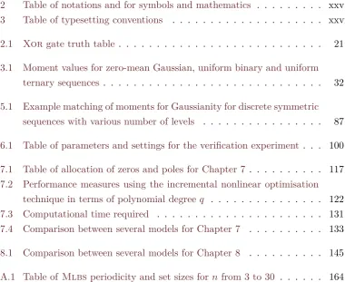
2 Table of notations and for symbols and mathematics . . . xxv

3 Table of typesetting conventions . . . xxvii

2.1 Xor gate truth table . . . 21

3.1 Moment values for zero-mean Gaussian, uniform binary and uniform ternary sequences . . . 32

5.1 Example matching of moments for Gaussianity for discrete symmetric sequences with various number of levels . . . 87

6.1 Table of parameters and settings for the veriﬁcation experiment . . . 100

7.1 Table of allocation of zeros and poles for Chapter 7 . . . 117

7.2 Performance measures using the incremental nonlinear optimisation technique in terms of polynomial degree 𝑞 . . . 122

7.3 Computational time required . . . 131

7.4 Comparison between several models for Chapter 7 . . . 133

8.1 Comparison between several models for Chapter 8 . . . 145

A.1 Table of Mlbsperiodicity and set sizes for 𝑛from 3 to 30 . . . 164

[image:13.595.117.498.254.565.2]

(14)

Acknowledgements

This thesis is dedicated to my Family, Friends and especially my Grandmother—

? _{A dwarf standing on the shoulder of a giant…—(Bernard of Chartres, 1159)} >

I very much appreciate the selﬂess support and kind encouragements oﬀered by my family and friends, without whom I would not be able to overcome so many failures and relish a few triumphs; for this I am eternally indebted. I am grateful to my good friends Natalie Ellis, Alice Ng, Hui Niu, Yuan Tian, Nami Morioka, Nixon Yu, Dan Zhou; my colleagues at both the University of Warwick and the Vrije Universiteit Brussel; Mr. Ho and his family at Rugby, and many others—unsung but not forgotten.

My sincerest gratitude goes to Professor Keith Godfrey and Professor Johan Schoukens, for being more than great mentors and treating me as a good friend. This endeavour would not have been possible without the technical guidance and emotional support by the two gentlemen; ‘a dwarf standing on the shoulder of two giants!’—to say otherwise is an understatement. I have to thank Keith again in par-ticular introducing and indulging me in much British culture, from visiting cathed-rals, the countryside, attending opera, ballets, orchestra and musicals to punting in horse races!

I would also like to thank Dr. Ai Hui Tan for her hospitality during our visit to the Multimedia University of Malaysia and the collaboration opportunities on the benchmark studies, it was a great honour. In addition, the invaluable suggestions and encouragements oﬀered by Professor Nigel Stocks were very much appreciated. Last but not least, many thanks to the members of the jury committee, administrative staﬀ and lawyers, all of whom went to extraordinary lengths to make the co-tuelle arrangements and the viva for the Ph.D. possible.

(15)

List of publications arising from this

research

Journal papers

Tan, A. H., Wong, H. K. & Godfrey, K. R. (2012, May). Identiﬁcation of a Wiener-Hammerstein system using an incremental nonlinear optimisation technique. Control Engineering Practice,20, 1140–1148.

Wong, H. K., Schoukens, J. & Godfrey, K. R. (2012a, March). Analysis of best linear approximation of a Wiener-Hammerstein system for arbitrary amplitude distributions.IEEE Trans. Instrum. Meas. 61(3), 645–654.

Wong, H. K., Schoukens, J. & Godfrey, K. R. (2013a). Design of multilevel signals for identifying the best linear approximation of nonlinear systems.IEEE Trans. Instrum. Meas. 62(2), 519–524.

Wong, H. K., Schoukens, J. & Godfrey, K. R. (2013b). Structured non-linear noise behaviour and the use of median averaging in non-linear systems with m-sequence inputs. IET Control Theory and Applications. [Accepted for Public-ation]. doi:10.1049/iet-cta.2012.0622

Conference papers with peer review

Wong, H. K. & Godfrey, K. R. (2010, September). A greybox approach to modelling a hyperfast switching Peltier cooling system. In Proc. UKACC International Conference on Control, 7th–10th September 2010 (pp. 1200–1205). Coventry, U.K.

Wong, H. K., Schoukens, J. & Godfrey, K. R. (2012b, September). Experimental veriﬁcation of best linear approximation of a Wiener system for binary

(16)

tions. InProc. UKACC International Conference on Control, 3rd–5th Septem-ber 2012 (pp. 941–946). Cardiﬀ, U.K.

Wong, H. K., Schoukens, J. & Godfrey, K. R. (2012c, July). The use of binary sequences in determining the best linear approximation of nonlinear systems. InProc. 16th IFAC Symposium on System Identiﬁcation, 11th–13th July 2012 (pp. 1323–1328). Brussels, Belgium.

(17)

Declarations

This thesis was submitted to the University of Warwick and Vrije Universiteit Brus-sel in partial fulﬁlment of the requirements for the Doctor of Philosophy co-tuelle agreement between the two universities. The work presented here is my own, except where speciﬁcally stated otherwise. The work was performed both in the School of Engineering at the University of Warwick under the supervision of Professor Nigel G. Stocks and Professor Emeritus Keith R. Godfrey, and in the Department of Fundamental Electricity and Instrumentation, Faculty of Engineering at the Vrije Universiteit Brussel under the supervision of Professor Johan Schoukens.

The benchmark study documented in Chapter 7 was a collaboration with Dr. Tan, Ai Hui of the Multimedia University, Cyberjaya, Malaysia.

(18)

Abstract

System identification is the art of modelling of a process (physical, biolo-gical, etc.) or to predict its behaviour or output when the environment condition or parameter changes. One is modelling the input-output relationship of a system, for example, linking temperature of a greenhouse (output) to the sunlight intensity (input), power of a car engine (output) with fuel injection rate (input). In linear systems, changing an input parameter will result in a proportional increase in the system output. This is not the case in a nonlinear system. Linear system identi-fication has been extensively studied, more so than nonlinear system identiidenti-fication. Since most systems are nonlinear to some extent, there is significant interest in this topic as industrial processes become more and more complex.

In a linear dynamical system, knowing the impulse response function of a system will allow one to predict the output given any input. For nonlinear systems this is not the case. If advanced theory is not available, it is possible to approximate a nonlinear system by a linear one. One tool is the Best Linear Approximation (Bla), which is an impulse response function of a linear system that minimises the output diﬀerences between its nonlinear counterparts for a given class of input. The

Bla is often the starting point for modelling a nonlinear system. There is extens-ive literature on the Bla obtained from input signals with a Gaussian probability density function (p.d.f.), but there has been very little for other kinds of inputs. A Bla estimated from Gaussian inputs is useful in decoupling the linear dynamics from the nonlinearity, and in initialisation of parameterised models. As Gaussian inputs are not always practical to be introduced as excitations, it is important to investigate the dependence of theBlaon the amplitude distribution in more detail. This thesis studies the behaviour of the Blawith regards to other types of signals, and in particular, binary sequences where a signal takes only two levels. Such an input is valuable in many practical situations, for example where the input actuator is a switch or a valve and hence can only be turned either on or oﬀ.

While it is known in the literature that the Bla depends on the amplitude distribution of the input, as far as the author is aware, there is a lack of compre-hensive theoretical study on this topic. In this thesis, the Blas of discrete-time time-invariant nonlinear systems are studied theoretically for white inputs with an

(19)

arbitrary amplitude distribution, including Gaussian and binary sequences. In doing so, the thesis offers answers to fundamental questions of interest to system engin-eers, for example: 1) How the amplitude distribution of the input and the system dynamics affect the Bla? 2) How does one quantify the difference between the

Bla obtained from a Gaussian input and that obtained from an arbitrary input? 3) Is the diﬀerence (if any) negligible? 4) What can be done in terms of experiment design to minimise such diﬀerence?

To answer these questions, the theoretical expressions for theBlahave been developed for both Wiener-Hammerstein (Wh) systems and the more general Vol-terra systems. The theory for theWhcase has been veriﬁed by simulation and phys-ical experiments in Chapter 3and Chapter 6respectively. It is shown in Chapter3

that the difference between the Gaussian and non-Gaussian Bla’s depends on the system memory as well as the higher order moments of the non-Gaussian input. To quantify this difference, a measure called the Discrepancy Factor—a measure of relative error, was developed. It has been shown that when the system memory is short, the discrepancy can be as high as 44.4%, which is not negligible. This justifies the need for a method to decrease such discrepancy. One method is to design a ran-dom multilevel sequence for Gaussianity with respect to its higher order moments, and this is discussed in Chapter5.

When estimating the Blaeven in the absence of environment and measure-ment noise, the nonlinearity inevitably introduces nonlinear distortions—deviations from the Blaspeciﬁc to the realisation of input used. This also explains why more than one realisation of input and averaging is required to obtain a good estimate of theBla. It is observed that with a speciﬁc class of pseudorandom binary sequence (Prbs), called the maximum length binary sequence (Mlbsor the m-sequence), the nonlinear distortions appear structured in the time domain. Chapter 4 illustrates a simple and computationally inexpensive method to take advantage this structure to obtain better estimates of the Bla—by replacing mean averaging by median averaging.

Lastly, Chapters7and 8document two independent benchmark studies sep-arate from the main theoretical work of the thesis. The benchmark in Chapter 7is concerned with the modelling of an electricalWh system proposed in a special ses-sion of the 15th_{International Federation of Automatic Control (}_Ifac_{) Symposium on} System Identiﬁcation (Sysid) 2009 (Schoukens, Suykens & Ljung, 2009). Chapter8

is concerned with the modelling of a ‘hyperfast’ Peltier cooling system ﬁrst pro-posed in the U.K. Automatic Control Council (Ukacc) International Conference on Control, 2010 (Control 2010).

(20)

Acronyms and Abbreviations

† _{Bold page numbers point to pages in which terms are deﬁned or explained in the} text.

Acronym Abbreviation Pages†

Adc Analogue-to-digital converter 98

Are Asymptotic relative (statistical) eﬃciency 75–77,82

Awgn Additive white Gaussian noise 15,58,62,65,78,82

Bla Best Linear Approximation ix, 4–9, 18,25,27, 28,

29–31, 33–39, 41–49,

51, 53, 55–58, 60, 63,

65, 66, 68–74, 76, 78–

80, 83, 86, 87, 91, 93–

95, 97, 99, 101, 103,

104,106–111,113–116,

123,132,145,147–151,

165,167,169–172,174,

176,184

Cf Crest factor 14,18,95,96

Df Discrepancy Factor 7,9,47,48–53,55,56,

86,87,91,92,148,150,

151

Dft Discrete Fourier transform 13, 14–16, 18, 19, 21,

23, 24, 59, 69, 73, 78,

129

Dirbs Discrete-interval Random Binary Sequence 15, 16, 17, 32, 33, 38,

49, 61–63, 65, 66, 69,

73,77,78,82–84

Dtft Discrete-time Fourier transform 12, 13

Fft Fast Fourier transform 20

Fir Finite impulse response 35, 39, 65, 66, 69, 77,

109,116,138

(21)

Frf Frequency response function 4, 13, 14, 27, 39, 69,

116

Ft Fourier transform 4,11,12,13,106

Hlle Hodges-Lehmann location estimator 77,78,82

Iir Inﬁnite impulse response 35, 39,77,80,84,109,

116

Irbs Inverse-repeat Binary Sequence 14, 24, 63, 65, 66, 68,

83

Irf Impulse response function 4, 13, 14, 27, 28, 35,

38, 41, 44–46, 49, 50,

52, 53, 55, 56, 65, 69–

71, 77, 78, 80, 82, 83,

106,109,172,175–177

Lfsr Linear feedback shift registers 19–21,23,24,163

Mae Mean absolute error 141,145

Miso Multiple-input single-output 135

Mlbs Maximum Length Binary Sequence 7, 9, 18, 19–25, 32,

33, 38, 39, 60, 61, 63,

65, 66, 68, 69, 71, 72,

74, 78–80, 82–84, 99,

100,103–105,107,108,

149–151,163,181

Mle Maximum likelihood estimator 82

Mse Mean squared error 62, 66,78,80–83, 112,

141,145

Oe Output-error (model/framework) 57,62

p.d.f. Probability density function xxiv,5, 15, 17, 18, 25,

47,75,86

Pi Periodicity-invariant (system) 11, 12, 15, 28, 34, 35,

165

Pips Performance Index for Perturbation Sequences 14,95,96

p.m.f. Probability mass function 5,25,47,86,88–90,95

Prbs Pseudorandom binary sequence 18,60,85

Prms Pseudorandom multilevel sequence 25,85

rms Root mean squared 33, 100,104, 106, 113,

114,116,182

Rse Relative statistical eﬃciency 74,75,76,82

Siso Single-input single-output 2,33,43,136

Snr Signal-to-noise ratio 9, 14, 16, 18, 62, 65,

77, 79,81–83, 95, 149,

151

(22)

Wh Wiener-Hammerstein (system) 7, 31, 33, 34, 43, 56,

86, 111,112, 115, 116,

125,132,133,147

Xor EXclusive-OR logic gate 20,21,24

Zoh Zero-order hold 16,23,53,99,101,102,

112

(23)

Glossaries

Blackbox model — In system identiﬁcation, the termblackboxmodelling refers to the process of modelling a system through non-parametric techniques, without knowledge of physical inner workings of the system, resulting in an empirical model. 8,112,136,138,145

dc stands for direct current in electrical engineering. Regardless of the physical nature of a signal (electrical or otherwise), the terms dc oﬀset, dc bias, dc term or dc component are all used widely in signal processing to refer to the mean value of a waveform in the time domain or the zero frequency component in the frequency domain. viii,15,16,19,23,24,34,38,39,43,66,125

ELiS stands for “Estimator for Linear Systems”, a program in the Frequency Do-main System Identiﬁcation (Fdident) toolbox forMatlab. It implements an iterative weighted nonlinear least squares procedure that ﬁts parametric mod-els to non-parametric transfer characteristics of dynamical systems (Kollár, 1994). 49,58,91,104,108,113,114,120,125,127

Empirical model — seeblackbox model

Galois is a program to generate pseudorandom signals including maximum-length sequences with various number of levels Barker (2008), Godfrey, Tan, Barker and Chong (2005). The signals can be designed to have desirable properties for dynamic system testing. 24,85

Gaussianity is a qualitative measure of how close the statistical distribution of a random variable is to a true Gaussian distribution, also known as a normal distribution. xviii,7,9,18,86,93,96

(24)

Greybox model — In system identiﬁcation, a greybox modelling approach is a mixture between whitebox and blackbox modelling. 136, see also blackbox model &whitebox model

Matlab (MATrix LABoratory) is a widely used scientiﬁc numerical computation environment developed by MathWorks with its own programming language. The platform is optimised for matrix and vector based calculations and oﬀer a wide range of tools for the manipulation, processing and visualisation of data.

xxii, xxiv,17,24,38,58,62,63,65,77,93,98,104,106, 113, 116, 121, 127,

129,137,146,181–183

Mechanistic model —see whitebox model

Moments — see deﬁnition on p.32. xxiii

Non-parametric model is a data-driven model without a priori speciﬁcation of a model structure; instead the structure is determined entirely from the data. Essentially the parameters are not ﬁxed and typically grow in size according to the amount of data available see. 30, 39, 49, 58, 68,91,93,104,106–108,

136

Parametric model is a problem-driven model with a ﬁxed model structure and a predetermined number of parameters. A good model can capture maximal useful information from the data used to derive it with only a few number of parameters. 49,91,104–108,See also non-parametric model

Probability density function (p.d.f.) — In probability statistics, a p.d.f. of a continuous random variable is a density function of 𝑥 such that, when integ-rated over a range of 𝑥 to give the area under the curve, the area describes the relative likelihood for ﬁnding this random variable to lie within that range at any given time. The p.d.f. deﬁnes the amplitude distribution and the mo-mentsfor the random variable. See alsomoments&probability mass function (p.m.f.)

Probability mass function (p.m.f.) — In probability statistics, a p.m.f. of a dis-creterandom variable is a discrete function of discrete variable𝑥that describes the relative likelihood for ﬁnding this random variable to take on a given value

𝑥 at any given time. The p.m.f. deﬁnes the distribution and themoments for the random variable. The p.m.f. for a discrete variable is the discrete analogue

(25)

of the continuous probability density function (p.d.f.). See also moments &

probability density function (p.d.f.)

prs stands for “pseudorandom sequences” and is a collection of programs written for Matlab software to generate maximum-length sequences and primitive polynomials in a convenient package (Tan & Godfrey, 2002). 24,85,181

Simulink is a commercial tool developed by MathWorks with a tight integration withMatlabsoftware that oﬀers a block-oriented multi-domain programming approach to modelling, stimulating and analysing dynamic systems (Krauss, Shure & Little, 1994). 137,138,146,see also Matlab

Uniform distribution — In probability statistics, a random variable 𝑥 with a uniform distribution has equal relative likelihood (or probability) of taking any permissible values. The uniform distribution may be discrete or continuous and is usually deﬁned by a range, for example, 𝑎 ≤ 𝑥 ≤ 𝑏. 17, 93, See also

moments, probability density function (p.d.f.) & probability mass function (p.m.f.)

Whitebox model — In system identiﬁcation, the term whitebox modelling refers to the process of modelling a system through ﬁrst principles, laws of physics and explicit assumed relationships between the input and output through prior knowledge of the system, resulting in a mechanistic model. 8,136,145

(26)

Mathematical notations and typesetting

conventions

Unless otherwise speciﬁed, notations for symbols and mathematics are as follows: Table 2: Table of notations and for symbols and mathematics

Symbol Description

≈ ...approximately equals to ...

≡ ...is a mathematical identity of ...

≜ ...by deﬁnition equals to...

∀ ...for all ...

𝜇 Arithmetic mean

𝜎 Standard deviation

𝑒 Euler’s number (Napier’s constant)

𝑓, 𝜔 Frequency variables (Hz, rad s )

f(𝑥) Generic function on𝑥

f(𝑥)_↦𝑦 f(𝑥)is deﬁned such that𝑥 maps to 𝑦

𝜋 Ratio of a circle’s circumference to its diameter

j Imaginary number, equals√−1

f(𝜃 ) = arg minf(𝜃) Speciﬁc value 𝜃 = 𝜃 that minimises f(𝜃) resulting in the

min-imised function of f(𝜃 ) 𝑔_Bla(𝑡) Bla (time domain)

𝐺_Bla(j𝜔) Bla (frequency domain)

𝑇 Sampling interval or bit-interval

𝑢(𝑡) Continuous input signal 𝑢 at time𝑡

𝑢[𝑘] Sampled input signal 𝑢 at sample 𝑘, 𝑘 counts from zero, i.e.

𝑢[0] = 𝑢(0 ≤ 𝑡 < 𝑇 )

continued on next page

(27)

continued from previous page

Symbol Description

𝑦(𝑡), 𝑦[𝑘] Similar deﬁnitions to𝑢(𝑡)and 𝑢[𝑘]respectively but for the out-put signal 𝑦instead of𝑢

ℱ{𝑥} The Dftof 𝑥

ℱ {𝑋} The inverse Dft of𝑋

𝒪 Big-O notation, describes the limiting behaviour of a function

𝒩(𝜇, 𝜎 ) Gaussian (normal) distribution of mean𝜇 and variance𝜎 𝒰(𝑎, 𝑏) Continuous uniform distribution between 𝑎and 𝑏

𝒰 Symmetrical discrete uniform distribution with𝑛 levels

𝑥 ∼ 𝒩 Random variable𝑥 follows a normal distribution

𝑥∈𝒗 𝑥 belongs to, or is a member of,𝒗 𝑥! The factorial of 𝑥

𝑥!! The double factorial of𝑥

E_J𝑥_K The expected value of the random variable 𝑥 {𝑥} A set of 𝑥

⟨𝑢⟩ A sequence of𝑢

𝒗 The transpose of vector 𝒗

𝑅_uu The autocorrelation function of the signal𝑢

𝑅_yu The cross-correlation function between the signals𝑦 and 𝑢 ℕ Set of natural numbers excluding zero

ℕ₀ Set of natural numbers including zero

|𝑥| Absolute value, magnitude or cardinality (set theory) of 𝑥 𝒂\𝒃 𝑎complement 𝑏(set theory)

𝒂 ⊂ 𝒃 𝑎is a proper subset of 𝑏(set theory)

𝒂 ⊆ 𝒃 𝑎is a subset of 𝑏 (set theory)

𝟙 (𝑥) The multiplicity function for multiset 𝑨 operating on element

𝑥 (set theory)

s s-domain operator

z z-domain operator

ℜ Real number axis

ℑ Imaginary number axis

𝑥| Expression 𝑥 applies given condition𝑎 = 1is satisﬁed

𝔇 Discrepancy Factor, see Section 3.5

𝔐 Notation for Moments, see Section 3.2

(28)

[image:28.595.107.496.141.370.2]

The conventions for typesetting are given are given in the following table:

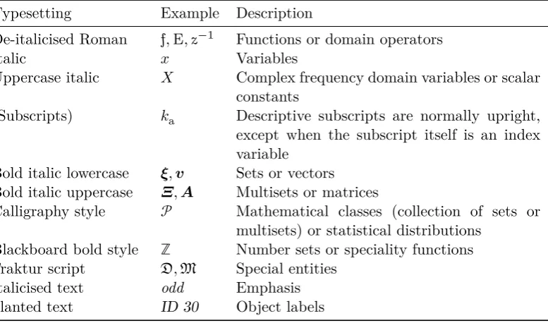
Table 3: Table of typesetting conventions

Typesetting Example Description

De-italicised Roman f,E,z Functions or domain operators

Italic 𝑥 Variables

Uppercase italic 𝑋 Complex frequency domain variables or scalar constants

(Subscripts) 𝑘_a Descriptive subscripts are normally upright, except when the subscript itself is an index variable

Bold italic lowercase 𝝃, 𝒗 Sets or vectors Bold italic uppercase 𝜩, 𝑨 Multisets or matrices

Calligraphy style 𝒫 Mathematical classes (collection of sets or multisets) or statistical distributions

Blackboard bold style ℤ Number sets or speciality functions Fraktur script 𝔇, 𝔐 Special entities

Italicised text odd Emphasis Slanted text ID 30 Object labels

(29)

(30)

C

1 Introduction

1.1 Background of System Identiﬁcation

The field of system identification and modelling is relatively modern. Before its gen-eralisation, systems science was born out of necessity from several different fields, for example, biomedicine, neuroscience, meteorology, signal processing, communica-tions, geology and acoustics. They all share a common goal: to create mathematical models capable of encapsulating some real processes and subsequently allow one to make prediction and, depending on application, control or influence the process to give certain desirable outcome.

1.1.1 Systems and models

(31)

1.1. Background of System Identiﬁcation

Similarly, in system and control theory, a system is a process with single or multiple inputs directly inﬂuencing or determining the quantity of a single or some combinations of outputs. System and control engineers sought to understand the relationships between these inputs and outputs, and therefore to make predictions or devise the best way to manipulate the inputs in order to attain certain desired output behaviour. Many systems studied are dynamical—their outputs at any given time simultaneously depend on more than one past instants of inputs, outputs, or a combination of both. In other words, the outputs of the immediate future are not just determined by the inputs or outputs at this very current moment, but also the values in past moments. Exhibiting dynamics is also called having memory eﬀects. In the frequency domain a dynamical system is characterised by having non-constant magnitude and phase frequency responses. A system without dynamics is called a static system.

A model of a system is a mathematical description of the relationships gov-erning the inputs and outputs. Such a model may contain a complete description or an approximation of the system. Unless full physical knowledge and the corres-ponding law of physics are well understood, it is usually not possible to devise a complete description. To be able to understand the relationship between the inputs and outputs, it is necessarily to apply techniques from the disciplines of system identification and modelling. Systemidentification is the art of extracting informa-tion and gathering data efficiently and accurately from the system in quesinforma-tion with certain user-specified goals. Sometimes it is possible to take control of an input, which simplifies the process. In such cases, the choice of the types and properties of input signals is important to the quality of information extracted. With data gathered, one can then start building models of the system. System modelling, on the other hand, is the art of choosing, developing and validating models that give the most accurate and precise description of the real system based on the finite measurement data obtained from system identification. A good model allows one to predict the output or outputs of a system given some arbitrary inputs, or at the very least, normal operating inputs expected for the real operation of the system. Once a model has been derived and validated, the foundation is set for control engineers to devise optimised control schemes to influence a system to achieve certain desired behaviour.

In this thesis, for simplicity, only dynamical systems with a single input and a single output are considered, these systems are referred to as input single-output (Siso) systems. The systems considered are also time-invariant. This is to say, the system dynamics, structure and behavior remain unchanged with time so

(32)

that under the same input and given the same initial conditions, the system always generates the same output.

1.1.2 Linear and nonlinear systems

Linear models are well documented and commonly used, even when the underlying system is nonlinear (Ljung, 1999, tbl. 4.1). The concept of linearisation and pro-portionality is well known and used in a wide range of fields. Some relationships in nature are predominantly linear, some are very nonlinear and there are those in between. All ‘linear’ systems are nonlinear to a certain extent—there are no true linear relationships, as ultimately the linearity breaks down at some extreme points due to changing law of physics or when external factors are introduced and starting to dominate. Even with moderately nonlinear systems, linear models of sufficient quality can be obtained given a small enough input domain or operation range. Mathematicians, scientists and engineers prefer to apply linear approxima-tions because their simplicity opens the door for closed-form algebraic study and allows models to be devised with minimal effort and cost.

Deﬁnition A nonlinear system is a system where the input-output relationship(s) does not obey the principle of superposition.

An example of a nonlinear system is the human auditory system—doubling the power output of a loudspeaker does not double the perceived loudness. It also has dynamics—diﬀerent loudness is also perceived for tones with diﬀerent frequencies. Note that in this thesis, the termnonlinear systemis used for a dynamical nonlinear system while the termstatic nonlinearity is used to refer a static nonlinear entity.

1.1.3 Impulse and impulse response

(33)

tensioned wires in the piano to be struck by hammers. Each key corresponds to a different wire that was taut with a specifically tuned tension force (or made with an entirely different metal), in order to have its resonant frequency corresponding to a particular musical note. The strike of the hammer is effectively an impulse that causes the struck wire to vibrate and resonate at its natural frequency. This vibra-tion interacts with the sound board of the piano and the surrounding air to produce the musical note as a perceivable sound. An example of successful application of impulses in a system identification problem is in the analysis of the acoustics of a concert hall though gunshots and even balloon bursts (Sumarac-Pavlovic, Mijic & Kurtovic, 2008).

With an impulse as excitation, it is possible to extract information of the dynamics from a system. The response as a function of time of a linear dynamical time-invariant system to an applied impulse is called the impulse response function (Irf), and is sufficient to describe the dynamics (but not the inner-structure) of a linear time-invariant dynamical system. Knowing the Irf allows one to predict the output of the system under any arbitrary inputs (not outside operating ranges that may induce nonlinear effects). Because of this, the objective of many system identification exercises is to obtain theIrf. Thefrequency response function (Frf)

is the analogue of the Irf in the frequency domain. Through the use of Fourier transform (Ft) there is a one-to-one mapping between the frequency domain and the time domain (see Section 2.2).

For nonlinear systems, the closest analogue of an Irf is the Volterra kernel (Volterra, 1930/2005), akin to a multidimensional Irf. This will be discussed in more detail in Section 3.4. However, it is possible to devise an Irf to represent a linear model that behaves, as close as possible, to a nonlinear system. One such tool is the Best Linear Approximation (Bla), introduced in the next section and discussed in more technical detail in Section 3.1.

1.1.4 The Best Linear Approximation (B)

To devise a model to fit the relationship of some data variates, firstly one has to define a measure of error between the model prediction and the true measured data, called the cost function. A popular choice is the least squares cost, where the total error is defined as the total squared differences between the model prediction and the true measurement. A model where this total error is minimised is called the least squares model. For example, in statistics, the ordinary least squares linear regression is a type of least squares model.

(34)

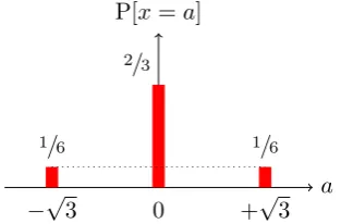
In dynamical systems, the least squares linear time-invariant model of a non-linear time-invariant system is called theBest Linear Approximation (Bla). It was founded on the basis of the Bussgang theorem (Bussgang, 1952) and it has several important properties under the influence of input signals having Gaussian p.d.f’s.: firstly, the transfer characteristics of a block-structured nonlinear system is the com-bined dynamics multiplied by certain constant factor depending on the nonlinearity (for example, see Section 3.3); and secondly, the Bla of a static nonlinearity is static. In this thesis, for convenience, the Bla obtained from signals bearing a Gaussianp.d.f. (orp.m.f. for discrete sequences) shall be called theGaussian Bla. However, the aforementioned properties do not apply if the inputs to the nonlinear system do not have a Gaussian distribution. Example 1.1 of Enqvist (2005) shows that the Bla of a static nonlinearity for non-Gaussian inputs is not necessarily static. Further, example 1.2 from the same source shows that the Bla can be different for two inputs despite sharing an equal colour (or power spectrum). A motivation example illustrating the dependence of the Bla on the amplitude distribution of the input signals is given as follows:

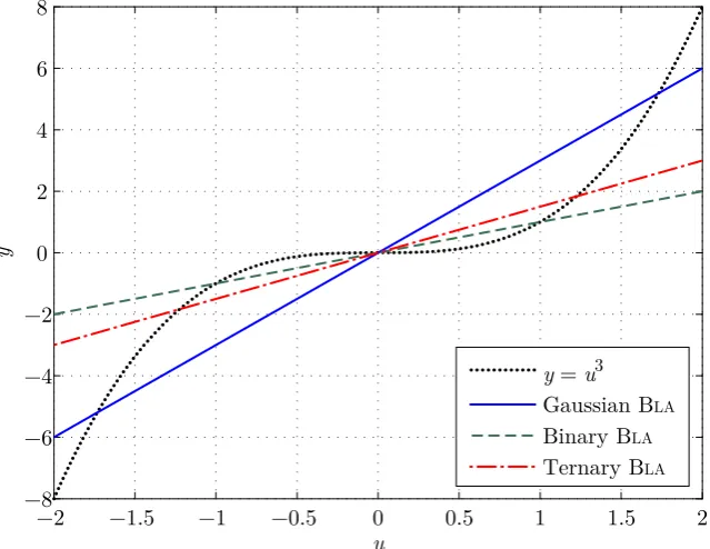
Example Consider a simple pure cubic nonlinearity such that the output 𝑦 is re-lated to the input 𝑢 by 𝑦 = 𝑢 , and hence there are no dynamics. Three types of zero-mean inputs: Gaussian, symmetrical (about zero) binary (2-level) sequences and symmetrical ternary (3-level) sequences are used to identify the Bla of the cubic nonlinearity. The binary and ternary sequences have their levels uniformly distributed, i.e. all their levels have equal probability of appearance, the value of which is / for the binary levels and / for the ternary levels. The power of all three sequences is normalised to unity. As a result, the variance of the Gaussian input is also unity. For the other two sequences, the power normalisation combined with the symmetry dictate that the binary sequence to comprise levels +1and −1

and the ternary sequence to comprise levels of+√1.5,0and−√1.5(see methods in Chapter5for the derivation). The results are shown in Fig.1.1. It can be seen that the Blas are indeed diﬀerent for all three types of inputs. This is understandable as the Blas are optimised to approximate the nonlinear cubic relationship to their best ability (in terms of least squared errors) within the range of input amplitudes of their corresponding input signal. This means that for the binary case, the Bla is exactly described by 𝑦 = 𝑢, as the error between 𝑦 = 𝑢 and 𝑦 = 𝑢 is exactly zero given input levels 𝑢 _∈ {+1, −1}. For the Gaussian case the Bla is 𝑦 = 3𝑢

(35)

1.2. Thesis outline

equal to the 4thorder moments of the corresponding input. The concept of moments will be introduced in Section 3.2 and within which, Table 3.1 contains the central moments for the three types of sequences used in this example.

−2 −1.5 −1 −0.5 0 0.5 1 1.5 2

−8 −6 −4 −2 0 2 4 6 8

y = u3 Gaussian BLA Binary BLA Ternary BLA

u

[image:35.595.140.460.179.426.2]

y

Figure 1.1: TheBlas of a static pure cubic nonlinearity identiﬁed by three types of input signals

As mentioned before, Gaussian Blashave desirable and well known proper-ties. However, in some systems, one cannot expect the inputs to have a Gaussian distribution—the flow rate of a fluid controlled by an on-off valve for example, is more binary in nature; this sets the motivation of the thesis. Questions arise, for example, what happens if a binary excitation is used instead of a Gaussian noise ex-citation? Will the results significantly change, or will the differences be sufficiently small that, for practical purposes, they can be ignored? Is it possible to quantify the differences between non-Gaussian and Gaussian excitations on the basis of the non-Gaussian measurement results? These questions will be addressed in Chapter3.

1.2 Thesis outline

This thesis is split into two parts containing nine chapters in total. The ﬁrst six chapters revolve around the main topic on the theory of the non-Gaussian Bla.

(36)

1.2. Thesis outline

Chapters 7 and 8 are both standalone chapters each documenting a benchmark study. The last chapter contains general conclusions, a discussion on future work and a summary of contributions. Details of each chapter in this thesis are listed as follows:

Chapter 2 introduces the various periodic input sequences used throughout this thesis with discussions on their properties and how they are generated.

The first part of Chapter 3 gives a formal definition of the Bla and shows that it is possible to derive closed-form expressions for the Blas obtained from signals with arbitrary amplitude distributions for any time-invariant discrete-time systems; within which two types of systems are shown: firstly the block-structured

Wiener-Hammerstein (Wh)system in Section3.3and secondly for the more general Volterra systems in Section3.4. The second part of Chapter3introduces a measure to quantify the diﬀerence called the Discrepancy Factor (Df) in Section 3.5. This answers the question on how much the Bla deviates from the Gaussian obtained counterpart and it is shown that systems with shorter memory, in general, have higherDfs.

The ﬁrst part of Chapter4introduces a method for identifying the Blaand discusses the behaviour of exogenous environment (and measurement) noise and nonlinear distortions arising from the nonlinearities, with respect to diﬀerent avail-able input sequences introduced in Section 2.3. The second part from Section 4.5

onwards documents a method to improve the estimates of the Bla through using alternative averaging schemes rather than the conventional mean function, by using a special property ofMaximum Length Binary Sequence (Mlbs)inputs resulting in structured nonlinear distortions. The results show such a method is simple to apply and eﬀective in low exogenous noise scenario.

Chapter 5illustrates a method to design discrete-interval random multilevel sequences for Gaussianity. Gaussian Bla has well documented properties, one of which is the ability to decouple the dynamics from the static nonlinear contributions. Some problems prohibit the use of continuous amplitude levels, examples of which are given in the beginning of the chapter. In such situations, optimising multilevel sequences for Gaussianityis one method to obtain an unbiased Gaussian Bla.

Chapter 6 details an experiment based on an electrical circuit in a Wiener system conﬁguration conducted to verify the discrete-time Bla theory developed in Chapter3, in which only simulated experiment was conducted. The experiment results successfully veriﬁed the theory in a laboratory setting.

(37)

1.3. Contributions

The content of this chapter is based on Tan, Wong and Godfrey (2012). The chapter shows a utilisation of one property of the Gaussian Bla—the Bla is proportional to the combined linear dynamics of the system. This allows a brute-force exhaustive search of all poles and zero combinations resulting in two physically realisable filters for the first and second linearities of a Wiener-Hammerstein system. The iterative algorithm proposed also models the static nonlinearity using a polynomial or a piecewise polynomial function. The parameters are tuned in multiple stages, first for linearity assignment, then to nonlinearity, to minimise the number of parameters the optimisation algorithm has to tackle at any stage. The polynomial degrees are increased one degree at a time to minimise the chance of the optimisation being stuck in a local minimum.

Chapter 8 documents a modelling exercise on a ‘hyperfast’ Peltier cooling system assembly (Cham, Tan & Tan, 2010). The solution encompasses a mixture of blackbox and whitebox modelling approaches, incorporating as much physical and structural knowledge of the system as possible and without relying on numer-ical non-parametric optimisation methods. The solution shows that even a simple, naïve approach that does not use established sophisticated system identiﬁcation methods, can yield models with acceptable performance given enough prior physical knowledge. This piece of work was based on Wong and Godfrey (2010).

1.3 Contributions

Much of the research documented in this thesis has previously been published in journal or conference publications; a list of which is available on p. xiv. Unless otherwise speciﬁed or referenced, all the work are performed by the author under the guidance of the supervisors named on p. ii with the exception of Chapter 7

which was part of a collaboration (see p.xvi). Major contributions arising from the research work performed over the course of this Ph.D. degree are highlighted in this section as follows:

The objective of this thesis is mainly concerned with the use of non-Gaussian signal in identifying theBlaof the system. While the dependence of theBlaon the input amplitude distribution is well known in the literature, the work in Chapter3, first published in Wong, Schoukens and Godfrey (2012a), tackles some questions rel-evant to the system identification community. To the best of the author’s knowledge, the effect of non-Gaussianity of inputs to the Blaof a time-invariant discrete-time nonlinear system has not been investigated in detail, and this thesis is able to provide closed-form algebraic expressions for the Bla of generalised discrete-time Volterra

(38)

1.3. Contributions

systems with arbitrary input distributions. This answers the question made in the beginning of the chapter: ‘What happens if a binary excitation is used instead of a Gaussian noise excitation?’. Another question is: ‘Will the results significantly change, or will the differences be sufficiently small that, for practical purposes, they can be ignored?’. The simulation experiments performed for a Wiener system with a) cubic (Section 3.3.1) and b) quintic (Section3.3.2) nonlinearity have shown that the Gaussian Bla and the Bla obtained from other input signals can have a sig-nificant difference between them. Finally, to answer: ‘Is it possible to quantify the differences between Gaussian and Gaussian excitations on the basis of the non-Gaussian measurement results?’, a measure called theDiscrepancy Factor(Df) was developed in Section3.5 to quantify the difference.

The first part of Chapter 4 discusses the behaviour of noise and nonlinear distortions and how it affects the choice of input signal. This piece of work was also published in Wong, Schoukens and Godfrey (2012c). In the second part, significant improvement to the quality of estimate of theBlaof a nonlinear system can be made when the input sequences used were Maximum Length Binary Sequences(Mlbs’s), giving rise to nonlinear distortions having a certain structure unique to Mlbs’s. While this structured behaviour is known in the literature, see for example, Godfrey and Moore (1974), Vanderkooy (1994), the structured nonlinear noise has been treated as a negative aspect rather than an opportunity. In this thesis, it was found that the use of alternative averaging schemes rather than the traditional mean-based averaging can offer significant improvement in the Blaestimate under moderate to high signal-to-noise ratio (Snr) due to the structured nonlinear distortions. The findings were submitted as Wong, Schoukens and Godfrey (2013b), which has been accepted for publication.

Another notable contribution involves the physical experiment performed to verify the theory developed in Chapter3, documented in Chapter6of this thesis and published in Wong, Schoukens and Godfrey (2012b). Here the experiment showed good agreement between the theory and practice.

(39)

1.3. Contributions

Netherlands.

Lastly, the benchmark Chapters of7and8document solutions to benchmark problems previously proposed in two separate conferences. The benchmark studies provided valuable training opportunities for the author in system identiﬁcation.

(40)

C

2 Periodic Input Sequences

P

eriodic sequences are widely used in system identification. They offer several advantages over aperiodic sequences in, for instance, eliminating spectral leakage (see Section 2.2), the ability to perform inter-period averaging to drive down the effect of exogenous environment noise (see Section 4.2) and allowing the user to compare the level of nonlinear distortions to that of noise (Pintelon & Schoukens, 2012). Several types of periodic input sequences used throughout this thesis are described in this chapter. Before these sequences are introduced in Section2.3, two concepts first explained: periodicity-invariant (Pi) property in Section 2.1 and the variousFourier transforms (Fts) in Section2.2.

2.1 Periodicity-invariance (Pi)

Deﬁnition A nonlinear system is designated as periodicity-invariant (Pi) when excited by any periodic input𝑢with period𝑁; the noise-free output𝑦would always share the same period𝑁.

(41)

2.2. Fourier transformations and periodicity

In this thesis, the focus is on periodic sequences due to several advantages highlighted in the next section, and as such all nonlinear systems considered are restricted to Pisystems.

2.2 Fourier transformations and periodicity

A signal is a carrier of information and it may take different physical forms: electrical such as voltage values; or mechanical such as the angle of a valve controlling the flow rate of some fluid. A signal can also be either continuous (in amplitude), an analogue signal; or discrete, a digital signal. Throughout this thesis, the termsequenceis used only to denote digital signals.

The spectral density of an infinitely long aperiodic continuous time signal not described by a finite sum of sinusoids is a continuous function of frequency, and is obtained by the continuousFourier transform (Ft). The Nyquist-Shannon sampling theorem states that the sampling frequency should be more than twice as high as the highest frequency content of a band-limited signal to be able to reconstruct the original signal with no loss of information. When an infinitely long analogue signal is sampled at fixed time intervals to create a sequence, with sampling frequency 𝑓_s(or sampling interval𝑇 = 1/𝑓_s) chosen to obey the Nyquist-Shannon sampling theorem, the spectral density is given by thediscrete-time Fourier transform (Dtft), defined for a sampled input𝑥[𝑘] as:

𝑋_Dtft(𝑒j _{) =} _{𝑥[𝑘]𝑒} j _(2.1)

where 𝑘 = 𝑛/𝑓_s for all integer 𝑛 ∈ ℤ. With respect to this equation, the Dtft manifests repeated spectral ‘copies’ of the Ft of the continuous signal, with each copy centred at frequencies 𝑛𝑓_s∀𝑛 ∈ ℤ. If one normalises the angular frequency variable from 𝜔 = 2𝜋𝑓, with units of radian per second, to 𝜔 ⟶ 2𝜋𝑓/𝑓_s = 2𝜋𝑓 𝑇, the periodicity of the 𝑋_Dtft over frequency then becomes exactly 1. Provided the Nyquist-Shannon theorem is satisfied, the overlapping or spectral aliasing between different copies is nil. In practice many signals are not truly band-limited and hence there is always a certain amount of aliasing; but with careful measurement strategy, e.g. with proper use of anti-aliasing filter, this can be minimised. In both cases the spectral density is a density function since the distribution is continuous over frequency and has dimension Hz .

In reality, it is a necessity to perform measurement in finite time. When a truncation of an infinite signal or sequence is made to create a finite data record,

(42)

2.3. Periodic input sequences

i.e. applying a rectangular time-window to obtain a snapshot, the record is assumed periodic when transferred to the frequency domain through the discrete Fourier transform (Dft), deﬁned as:

𝑋_Dft(𝑘) = 𝑥[𝑛]𝑒 j (2.2)

for𝑘 = 0, 1,..., 𝑁 − 1. The principal diﬀerence betweenDftand Ft/Dtftis that the Dft𝑋_Dft(𝑘) is always discrete in frequency. By imposing the input 𝑥 to have a periodicity of 𝑁,𝑋_Dft(𝑘)in essence becomes the 𝑁-point sampled version of the

𝑋_Dtft around the unit circle in the complex plane, at the points 𝜔 = (2𝜋𝑘/𝑁). This results in a power spectrum containing a discrete number of frequency lines, rather than power spectral density. Power spectrum is dimensionless in terms of time (i.e. involves only the unit of measurement, but not Hertz). If the original signal is aperiodic, theDftis only an approximation due to spectral leakage caused by truncation. Diﬀerent windowing functions such as the Hanning (named after Austrian meteorologist Julius von Hann) window are traditionally used instead of the rectangular window (simple truncation) to improve the estimate (Blackman & Tukey, 2012). In the case of periodic signals, the Poisson summation formula (developed by French mathematician Siméon Denis Poisson) also shows that the periodic summation of a function in the time domain is described completely by discrete samples of its Fourier transform. The converse is also true—the periodic summation of a function in the frequency domain is described completely by discrete samples of the original function in the time domain (Pinsky, 2002). Hence, in such cases, both the time domain and frequency domain functions are periodic and contain an equivalent description of one another.

In addition to linking a signal or sequence to its power spectrum,Ftsare also used for transforming an impulse response function (Irf) (see Section1.1.3) in the time domain to itsfrequency response function (Frf)frequency domain counterpart. If the Dft is used, the resulting Frf 𝐺(z) is valid for predicting the output of a discrete-time dynamical system𝑌(z) = 𝐺(z)𝑈(z)when subjected to discrete-interval periodic input excitation 𝑈(z), in steady-state.

2.3 Periodic input sequences

(43)

depend-2.3. Periodic input sequences

ing on its nature. For example, one only has a limited control on the concentration of a drug in a patient. In many problems however, the input signal is only restric-ted by the maximum amplitude limits of an actuator or by the maximum power a system can handle without its integrity being compromised.

There are two important properties that make an input signal viable for sys-tem identification for linear syssys-tems. Firstly, a signal must be ‘persistently exciting’ (see Shimkin & Feuer,1987; Söderström & Stoica, 1989, def. 5.1) such that the Irf or Frf can be extracted through mathematical operations; and secondly, a signal should contain maximal spectral content (or power) in the frequency band of in-terest to maximise thesignal-to-noise ratio (Snr)of the estimates, and with enough frequency resolution to discern between features of interest, for example, sharp res-onances. The impulse, introduced in Section 1.1.3, is a persistently exciting white signal that contains equal energy content in all frequencies. Impulses however, have a major disadvantage—being a signal that lasts only a very short period of time, the energy transmitted to the system-under-test is limited. When the environment has significant background noise, the impulse response can be overwhelmed and buried by noise, leading to a poor quality measurement. There are many metrics to quantify the suitability of signals for noisy linear system identification, two of which are crest factor (Cf) and Performance Index for Perturbation Sequences (Pips)

(see Schoukens, Pintelon, van der Ouderaa & Renneboog, 1988; Godfrey, Barker & Tucker,1999; Pintelon & Schoukens,2012, and also Section5.4). For nonlinear sys-tem identiﬁcation, it can be useful to intentionally suppress spectral lines to gauge the degree of nonlinearity distortions or to minimise them; one example is shown by using the Inverse-repeat Binary Sequence (Irbs)with odd-harmonics suppressed in Section4.4.

Rather than concentrating the energy in one burst in a short time window, many excitation signals continuously transfer energy into the system, limited only by actuator amplitude or the system energy balance (to avoid overheating, breakdown, etc.). Such signals are now a preference over impulses due to the higherSnr achiev-able. Thanks to the development of electronics such as digital-to-analogue con-verters, computers, signal processing algorithms, eﬃcient implementation of Four-ier transform algorithms such as the fast FourFour-ier Transform (Fft), more complex signals can be precisely and reliably generated, and measurement results can be interpreted with suﬃcient computing power.

In this section, several types of sequences mentioned in this thesis are intro-duced. The use of periodic sequences has an advantage in that theDftis completely immune to spectral leakage if the sequence was sampled at precisely the right time

(44)

points, (i.e. at the correct frequency) to create records of a complete period. An-other advantage is that transient eﬀects are easy to minimise or eliminate during measurement. Because of these advantages, periodic sequences should be used as excitations for system identiﬁcation of Pi systems wherever possible. All of the discrete-time excitations considered in this thesis are periodic. Zero-mean or near zero-mean sequences are used and therefore thedclevel (zeroth frequency) is either exactly or approximately zero.

Note that in this thesis, where a periodic discrete-interval sequence is said to have a period of 𝑁, the unit is in samples. This gives a period in seconds of𝑁𝑇, where 𝑇is the bit-interval of the signal generator in seconds. For the speciﬁcation of periods hereinafter, the units may be omitted; 𝑁𝑇 seconds and 𝑁 samples are used interchangeably.

2.3.1 White Gaussian noise

Aperiodic white Gaussian noise is a typical signal used in modelling environment and measurement noise, in which case the acronym Awgn for additive white Gaussian noise, is often used in the literature. The term ‘white’ refers to the fact that the power spectral density of the signal has a flat expected power in all frequencies within a certain frequency band of interest—an infinite bandwidth signal does not exist in reality, as such a signal would have infinite energy due to the infinite spectral content. Nevertheless such a mathematical model usually suffices to model a broadband (wide spectrum) noise that is white as far as the band of frequency of interest is concerned. The term Gaussian refers to the amplitude distribution or the probability density functions (p.d.f’s.) of finding the signal level at any given time as being normally distributed.

Periodic white Gaussian noise may be utilised as excitation signals for system identification. A discrete-interval white Gaussian noise sequence can be obtained when the noise is sampled at fixed time intervals. When the sequence is truncated into multiple records and each of which is made periodic, the magnitudes of their Dft spectra are stochastic. TheDftpower spectrum of each record is not strictly white, but after sufficient averaging of many records, the ensemble power spectrum tends to a white spectrum (see Section 4.3).

2.3.2 Discrete-Interval Random Binary Sequences (D's)

(45)

example, Godfrey (1980). If the high and low levels are chosen to be +𝑉 and −𝑉

respectively, the expected value of such a sequence is zero. Dirbs’s are aperiodic, and as their length approaches inﬁnity, their autocorrelation functions are asymp-totically equal to:

𝑅_uu[𝑘] = 𝑉 𝑘 = 0

0 𝑘 ≠ 0 (2.3)

Through truncation and splitting into records of length 𝑁, periodic Dirbs’s can be obtained, reaping the benefits associated with periodic sequences in terms of eliminating spectral leakage and allowing for inter-period averaging to reduce the output noise variance. They are not as useful for linear system identification as other sequences because of the need either to use a very large value of 𝑁 in order for their off-peak autocorrelation function to be small, or equivalently, by using a large number𝑀of different segment realisations with a much smaller value of𝑁and then averaging the results; in either case, a relatively long experimentation time is needed. If 𝑀is not large, then it is possible for theDft at some of the harmonics to be relatively small, resulting in a low Snrat those frequencies—this is discussed in more detail in Section 4.3.

0 20 40 60 80 230 250

−50 −40 −30 −20 −10 0

Frequency line

Power (dB)

10log

Figure 2.1: Dftpower spectrum of a typical periodicDirbs of period 𝑁 = 511

with levels±1

Periodic Dirbs’s have similar Dft spectral properties as periodic white Gaussian noise sequences introduced in the previous section. The power spectrum on a decibel (dB) scale of a typicalDirbsof length𝑁 = 511is presented in Fig.2.1. When taken as a whole, theDftpower spectra for a family of zero-meanzero-order hold (Zoh) Dirbs’s with power normalised to unity and period𝑁 have zero power indc(zero frequency or the constant term); the remaining power (of unity) is evenly