On reducing the effect of covariate factors in gait recognition : a classifier ensemble method

http://wrap.warwick.ac.uk

Original citation:

Guan, Yu, Li, Chang-Tsun and Roli, Fabio. (2014) On reducing the effect of covariate

factors in gait recognition : a classifier ensemble method. IEEE Transactions on Pattern

Analysis and Machine Intelligence (Number 99). ISSN 0162-8828

Permanent WRAP url:

http://wrap.warwick.ac.uk/64465

Copyright and reuse:

The Warwick Research Archive Portal (WRAP) makes this work of researchers of the

University of Warwick available open access under the following conditions.

This article is made available under the Creative Commons Attribution 3.0 (CC BY 3.0)

license and may be reused according to the conditions of the license. For more details

see:

http://creativecommons.org/licenses/by/3.0/

A note on versions:

The version presented in WRAP is the published version, or, version of record, and may

be cited as it appears here.

On Reducing the Effect of Covariate

Factors in Gait Recognition:

A Classifier Ensemble Method

Yu Guan, Chang-Tsun Li,

Senior Member, IEEE

, and

Fabio Roli,

Fellow, IEEE

Abstract—Robust human gait recognition is challenging because of the presence of covariate factors such as carrying condition, clothing, walking surface, etc. In this paper, we model the effect of covariates as an unknown partial feature corruption problem. Since the locations of corruptions may differ for different query gaits, relevant features may become irrelevant when walking condition changes. In this case, it is difficult to train one fixed classifier that is robust to a large number of different covariates. To tackle this problem, we propose a classifier ensemble method based on the random subspace nethod (RSM) and majority voting (MV). Its theoretical basis suggests it is insensitive to locations of corrupted features, and thus can generalize well to a large number of covariates. We also extend this method by proposing two strategies, i.e., local enhancing (LE) and hybrid decision-level fusion (HDF) to suppress the ratio of false votes to true votes (before MV). The performance of our approach is competitive against the most challenging covariates like clothing, walking surface, and elapsed time. We evaluate our method on the USF dataset and OU-ISIR-B dataset, and it has much higher performance than other state-of-the-art algorithms.

Index Terms—Classifier ensemble, random subspace method, local enhancing, hybrid decision-level fusion, gait recognition, covariate factors, biometrics

Ç

1

INTRODUCTION

COMPARED with other biometric traits like fingerprint or iris, the most significant advantage of gait is that it can be used for remote human identification without subject cooperation. Gait analysis has contributed to convictions in criminal cases in some countries like Denmark [1] and UK [2]. However, the performance of auto-matic gait recognition can be affected by covariate factors such as carrying condition, camera viewpoint, walking surface, clothing, elapsed time, etc. Designing a robust system to address these prob-lems is an acute challenge. Existing gait recognition methods can be roughly divided into two categories: model-based and appear-ance-based approaches. Model-based methods (e.g., [3]) employ the parameters of the body structure, while appearance-based approaches extract features directly from gait sequences regardless of the underlying structure. This work falls in the category of appearance-based methods, which can also work well on low-qual-ity gait videos, when the parameters of the body structure are diffi-cult to estimate precisely.

The average silhouette over one gait cycle, known as gait energy image (GEI), is a popular appearance-based representation [4]. The averaging operation encodes the information of the binary frames into a single grayscale image, which makes GEI less sensitive to segmentation errors [4]. Several GEI samples from the USF dataset [5] are shown in Fig. 1. Recently, Iwama et al. evaluated the effec-tiveness of several feature templates on a gait dataset consisting of more than 3,000 subjects. They found that good performance can be achieved by directly matching the GEI templates, when there are no covariates [6]. However, it is error-prone when covariates

exist. Therefore, many researchers have been formulating various feature descriptors to capture discriminant information from GEIs to deal with different covariates. In [4], Han and Bhanu utilized principle component analysis (PCA) and linear discriminant analy-sis (LDA) to extract features from the concatenated GEIs. To extract gait descriptors, Li et al. proposed a discriminant locally linear embedding (DLLE) framework, which can preserve the local mani-fold structure [7]. By using two subspace learning methods, cou-pled subspaces analysis (CSA) and discriminant analysis with tensor representation (DATER), Xu et al. extracted features directly from the GEIs [8]. They demonstrated that the matrix representa-tion can yield much higher performance than the vector repre-sentation reported in [4]. In [9], after convolving a number of Gabor functions with the GEI representation, Tao et al. used the Gabor-filtered GEI as a new gait feature template. They also pro-posed the general tensor discriminant analysis (GTDA) for feature extraction on the high-dimensional Gabor features [9]. To preserve the local manifold structure of the high-dimensional Gabor fea-tures, Chen et al. proposed a tensor-based Riemannian manifold distance-approximating projection (TRIMAP) framework [10]. Since spatial misalignment may degrade the performance, based on Gabor representation, Image-to-Class distance was utilized in [11] to allow feature matching to be carried out within a spatial neighborhood. By using the techniques of universal background model (UBM) learning and maximum a posteriori (MAP) adapta-tion, Xu et al. proposed the Gabor-based patch distribution feature (Gabor-PDF) in [12], and the classification is performed based on locality-constrained group sparse representation (LGSR). Com-pared with GEI features (e.g., [4], [8]), Gabor features (e.g., [9], [11], [12]) tend to be more discriminant and can yield higher accuracies. However, due to the high dimension of Gabor features, these meth-ods normally incur high computational costs.

Through the “cutting and fitting” scheme, synthetic GEIs can be generated to simulate the walking surface effect [4]. In [13], the population hidden Markov model was used for dynamic-normalized gait recognition (DNGR). Both methods can yield encouraging performance against the walking surface covariate. In [14], Wang et al. proposed chrono-gait image (CGI), with the temporal information of the gait sequence encoded. Although CGI has similar performance to GEI in most cases [6], [14], it outperforms GEI in tackling the carrying condition covariate [14]. In [15], through fusing gait features from different cameras, it was found that short elapsed time does not affect the perfor-mance significantly in a controlled environment. Clothing was instead deemed as the most challenging covariate [15]. Based on a gait dataset with 32 different clothes combinations, Hossain et al. proposed an adaptive scheme for weighting different body parts to reduce the effect of clothing [16]. Yet it requires an additional training set that covers “all” possible clothes types, which is less practical in real-world applications.

Most of the previous works have satisfactory performance against some covariates like carrying condition, shoe type, (small changes in) viewpoint, etc. However, so far it still remains anopen

question to tackle covariates like walking surface, clothing, and elapsed time inless controlled environments. As such, our aim is not only to build a general framework that can generalize to a large number of covariates in unseen walking conditions, but also to address these open issues. Based on GEIs, we model the effect caused by various covariates as an unknown partial feature corrup-tion problem and propose a weak classifier ensemble method to reduce such effect. Each weak classifier is generated by random sampling in the full feature space, so they may generalize to the unselected features in different directions [17]. This concept, named random subspace method (RSM), was initially proposed by Ho [17] for constructing decision forests. It was successfully applied to face recognition (e.g., [18]). In our previous works [19],

Y. Guan and C.-T. Li are with the Department of Computer Science, University of Warwick, Coventry, CV4 7AL, United Kingdom

E-mail: [email protected], [email protected].

F. Roli is with the Department of Electrical and Electronic Engineering, University of Cagliari, 09123, Cagliari, Italy. E-mail: [email protected].

Manuscript received 29 Apr. 2014; revised 28 Aug. 2014; accepted 27 Oct. 2014. Date of publication 0 . 0000; date of current version 0 . 0000.

Recommended for acceptance by S. Sarkar.

For information on obtaining reprints of this article, please send e-mail to: reprints@ieee. org, and reference the Digital Object Identifier below.

Digital Object Identifier no. 10.1109/TPAMI.2014.2366766

[20], we employed this concept in gait recognition. Empirical results suggested RSM-based classifier ensemble can generalize well to several covariates. However, more theoretical findings and experimental results are needed to support this gait recognition method, especially on addressing the aforementioned open issues. Our contributions in this work can be summarized as follows:

1) Modelling of gait recognition challenges.Based on GEIs, we model the effect of different covariates as a partial feature corruption problem with unknown locations.

2) Classifier ensemble solution and its extensions.Through ideal cases analysis, we provide the theoretical basis of the pro-posed classifier ensemble solution. To tackle the hard prob-lems in real cases, we further propose two strategies, namely, local enhancing (LE) and hybrid decision-level fusion (HDF).

3) Performance and open issues solving.On the USF dataset, our method has more than 80 percent accuracy, more than 10 percent higher than the second best. It has very competitive performance against covariates such as walking surface and elapsed time. On the OU-ISIR-B dataset, the 90 percent plus accuracy suggests our method is robust to clothing. 4) Parameters and time complexity. Our method only has a

few (i.e., 3) parameters, and the performance is not sen-sitive to them. Our method also has low time complex-ity. On the USF dataset, with the high-dimensional Gabor features, the training time can be within several minutes while the query time per sequence can be less than 1 second.

The rest of this paper is organized as follows, Section 2 dis-cusses the gait recognition challenges, and provides classifier ensemble solution and its extensions. Details of the random sub-space construction, local enhancing, and hybrid decision-level fusion are provided in Section 3, 4, and 5. Our method is experi-mentally evaluated and compared with other algorithms in Section 6. Section 7 concludes this paper.

2

PROBLEM

MODELLING AND

SOLUTION

Metric-learning methods are popular for gait recognition. The learned metrics (e.g., in [4], [7], [8], [9], [10], [21], [22], [23]), used as feature extractors, may reduce the effect of covariates to some extent. However, an effective metric can only be learned based on representative training set, while this assumption may not hold in real-world scenarios. Since most of the walking conditions of query gaits are unknown, the training set collected in normal condition cannot represent the whole population. In this case, overfitting may occur. To build a model that generalizes to unknown covari-ates, in this section we first model the effect of covariates as a par-tial feature corruption problem with unknown locations, and then we provide the theoretical analysis of the proposed RSM-based classifier ensemble solution and its extensions.

2.1 Gait Recognition Challenges

We model the effect of covariates by difference images between the probe and gallery. Given a subject with the gallery GEIIgallery, and

the probe GEIs fI_iprobegF_i¼1 inF different walking conditions, we define the corresponding difference images as:

^

Ii¼Iprobei I

gallery_{; i2 ½1; F; (1)}

as shown in Fig. 2. Several examples of_I^_{icorresponding to} differ-ent walking conditions are also illustrated in Fig. 3. For an unknown walking conditioni,I^i indicates the corrupted gait

fea-tures with unknown locations. Before matching, we need to find a feature extractorTthat can suppressI^i, i.e.,

T¼argminkI^iTk2; i2 ½1; F; (2)

where T can extract features in the column direction of ^

Ii. However, the locations of corruptions may differ for

differ-ent walking conditions, as shown in Fig. 3. Given such non-deterministicnature ofI^i, from (2) we can see that it is difficult

to find afixedT that can extract effective features that can gen-eralize to a large number of different covariates. In light of this, an effectiveT should only extract the relevant features dynami-callyfor different walking conditions.

2.2 Problem Formulation

For high dimensional gait feature templates, PCA is usually used for dimension reduction (e.g., [4], [14]). In this work, we instead use the matrix-based two-dimensional PCA (2DPCA) [24] because of its lower computational costs and higher performance.

LetT be the 2DPCA transformation matrix consisting of the leadingdnon-zero principle components such thatT ¼ ½t1; t2;. . .;

td. Since½t1; t2;. . .; tdare pairwise orthogonal vectors, (2) can be

written as:

T¼argminX

d

j¼1

k_I^

itjk2; i2 ½1; F: (3)

It is difficult for traditional 2DPCA with a fixedT¼ ½t1; t2;. . .; td

to reduce the effect ofF different walking conditions. In (3), since the termskI^itjk2; j2 ½1; dare non-negative, it is possible to reduce

the effect of covariates by selecting a subset of½t1; t2;. . .; tdto form

a new feature extractor.

To see the reduced effect of covariates, we form different feature extractors by randomly selecting 2 projection directions from ½t1; t2;. . .; td. In Fig. 4, we report the corresponding normalized

Fig. 2. An example of modelling the covariate effect by image difference between the gallery GEI (i.e., Fig. 1a) and a probe GEI (i.e., Fig. 1e).

Fig. 3. From left to right: difference images between the gallery GEI Fig. 1a and the probe GEIs Figs. 1b, 1c, 1d, 1e, 1f, 1g.

Fig. 4. Normalized Euclidean distances from gallery sample Fig. 1a to probe sam-ples Figs. 1b, 1c, 1d, 1e, 1f, 1g, based on different projection directions.

Euclidean distances from the gallery sample in Fig. 1a to the probe samples in Figs. 1b, 1c, 1d, 1e, 1f, 1g, respectively. We can see the effect of covariates in Fig. 1b/Fig. 1e can be reduced by using ½t2; t35, while the effect in Fig. 1g can be reduced based on½t15; t61.

These observations empirically validate that it is possible to select subsets of½t1; t2;. . .; tdas feature extractors to reduce the effect of

covariates. However, the optimal subset may vary for different walking conditions due to thenon-deterministicnature ofI^i.

Therefore, we formulate the problem of reducing the effect of unknown covariates as adynamicfeature selection problem. For an unknown walking condition, we assume the irrelevant fea-tures (mainly corresponding to the corrupted pixels, as indi-cated by_I^_{i) exist inmð0< m < dÞunknown non-negative terms} of (3). We aim to dynamicallyselect N2 ½1; d relevant features (mainly corresponding to the uncorrupted pixels) for classifica-tion. It is obvious that the probability of selectingNrelevant fea-tures is 0 when N > dm. When N2 ½1; dm, by randomly selecting N features out of d features, the probability of not

choosing the mirrelevant features PðNÞfollows the hypergeo-metric distribution [25]. This can be expressed as the ratio of binomial coefficients:

PðNÞ ¼

dm N

dðdmÞ NN

d N

¼ðdmÞ!ðdNÞ!

d!ðdmNÞ! ; N2 ½1; dm: (4)

PðNÞis a generalization measure that is related in someway to the performance of the matching algorithm. Classifiers with greater PðNÞtend to generalize well to unseen covariates, and vice versa.

Lemma 1.Letd; m; Nbe the numbers of the total features, irrelevant fea-tures (with0< m < d), and randomly selected features, respectively, then PðNÞ in (4) is inversely proportional to N in the range N2 ½1; dm.

Proof.It can be proved using mathematical induction. From (4), it is easy to see that PðNþ1Þ=PðNÞ ¼1m=ðdNÞ<1 for N2 ½1; dm. This completes the proof of the lemma. tu

It is preferable to set N to smaller values, which can yield greater PðNÞ, according to Lemma 1. Specifically, when Nd, the hypergeometric distribution can be deemed as a binomial dis-tribution [25], we have

PðNÞ ¼ N N p

N_ð1pÞðNNÞ_¼pN_{; Nd; (5)}

wherepis the probability of randomly selecting one relevant fea-ture. Sincep¼1m=d, (5) can be written as:

PðNÞ ¼ 1m d

N

; Nd; (6)

which clearly reflects the simple relationship betweenPðNÞand the other parameters when we setNd.

2.3 Classifier Ensemble Solution and its Extensions We use a classifier ensemble strategy for covariate-invariant gait recognition. After repeating the random feature selection processL times (Lis alarge number),Lbase classifiers with generalization abilityPðNÞ(see (6)) are generated. Classification can then be per-formed by majority voting (MV) [26] among the labeling results of the base classifiers.

Given a query gait and the gallery consisting of cclasses, we define the true votesVtrueas the number of classifiers with correct

prediction, while the false votesfVi falseg

c1

i¼1 as the incorrectly

pre-dicted classifier number distribution over the otherc1 classes. Given that, through MV, the final correct classification can be achieved only whenVtrue>maxfVfalsei g

c1 i¼1.

Ideal cases analysis.We make two assumptions in ideal cases:

1) When irrelevant features are not assigned to a classifier (referred to as unaffected classifier), correct classification should be achieved.

2) When irrelevant features are assigned to a classifier (referred to asaffected classifier), the output label should be a random guess from thecclasses, with a probability of1=c. GivenLclassifiers, in the ideal cases the true votesVtruecan be

approximated as the sum of the number of unaffected classifiers PðNÞL(based onthe law of large numbers[27]) and the number of

affected classifiers:

Vtrueround PðNÞLþ

ð1PðNÞÞL c

!

: (7)

Similarly, in the ideal cases the false votes should correspond to the number ofaffected classifiers for the otherc1 classes. Based on assumption 2), its maximum value,maxfVi

falseg c1

i¼1, can be roughly

expressed as the corresponding mean value:

maxV_falsei c_i¼1₁meanV_falsei c_i¼11round ð1PðNÞÞL c

! : (8)

Correct classification can be achieved whenVtrue>maxfVfalsei g c1 i¼1.

From (7) and (8), it is obvious that this condition can be met when PðNÞ> "("is a small positive number).

From ideal cases analysis, it can be seen that weonly careabout the number of unaffected classifiers, instead of which ones are. According to (6), by settingNto a small number to makePðNÞ> ", the corresponding classifier ensemble methodis insensitive to the locations of corrupted features (since _Vtrue>maxfVi

falseg c1

i¼1, as supported by (7) and (8)).

Therefore, it is robust to a large number of covariates as long as the irrele-vant feature number is not extremely large (i.e.,m < din (6)).

Real cases analysis.Here the two assumptions made in the ideal cases analysis do not hold precisely: 1)unaffected classifiersdo not always make the correct classification; 2) although theaffected classi-fierswould result in label assigning in a relatively random manner, it is difficult to estimatemaxfVi

falseg c1

i¼1 precisely. However, in real

cases we can deemVtrueandmaxfVfalsei g c1

i¼1 from ideal cases

analy-sis as the upper bound and lower bound, respectively, i.e.,

VtrueVtrue;

maxVi false

c1

i¼1 maxfV i falseg

c1 i¼1:

(9)

Since correct classification can be achieved only when Vtrue>

maxfVi falseg

c1

i¼1, our objective is to increase Vtrue and decrease

maxfVi falseg

c1

i¼1. Since it is difficult to estimate maxfVfalsei g c1 i¼1

pre-cisely, we relax the objective by decreasingPci¼11Vfalsei . Then we

can reformulate our objective as a problem of suppressing G defined as

G¼ Pc1

i¼1V i false

Vtrueþ

; (10)

whereis a small positive number to avoid trivial results. To sup-pressGin (10), we extend the classifier ensemble method by pro-posing two strategies:

1) Local enhancing.If we use the output labels of all theL classi-fiers as valid votes such thatL¼Vtrueþ

Pc1

i¼1Vfalsei , then according

to (10) we can getG/L=ðVtrueþÞ:SinceLis a constant, the first

strategy is to increaseVtrue. To realize it, based on supervised

2) Hybrid decision-level fusion.The second strategy is to decrease Pc1

i¼1V i

falsebydynamicallyeliminating classifiers corresponding to

the irrelevant features, before MV. Irrelevant features would lead to label assignment in a relatively random manner. Based on the

same irrelevant features, a classifier pair corresponding to two

differentLE methods would produce two random labels, which are unlikely to be the same. Based on the “AND” rule, classifier pairs with different output labels are deemed as invalid votes and sim-ply discarded. Although this scheme may also decrease Vtrue to

some extent, it significantly reduces the value ofPci¼11Vfalsei to

sup-pressGin (10). Details of HDF are presented in Section 5.

3

RANDOM

SUBSPACE

CONSTRUCTION

We construct the feature space using 2DPCA, from which we can generate Lfeature extractors. Given ngait templates (e.g., GEIs) fIi2RN1N2gni¼1 in the training set (i.e., the gallery), we can

com-pute the scatter matrix S¼1 n

Pn

i¼1ðIimÞTðIimÞ, where m¼ 1

n

Pn

i¼1Ii. The eigenvectors ofScan be calculated, and the leading

d eigenvectors associated with non-zero eigenvalues are retained as candidates T ¼ ½t1; t2;. . .; td 2RN2d to construct the random

subspaces. By repeatingLtimes the process of randomly selecting subsets of T (with size Nd), the random subspaces fRl_2RN2NgL

l¼1are generated and can be used as random feature

extractors. Then a gait templateI2RN1N2_{can be represented as a}

set of random featuresfXl_2RN1NgL

l¼1such that

Xl¼IRl; l¼1;2;. . .; L: (11)

Note the random feature extraction is only performed in the col-umn direction ofI, with the dimension reduced toRN1N_.

4

LOCAL

ENHANCING

The random features can be used for classification directly. How-ever, these features may be redundant and less discriminant since 1) the random feature extraction process based on (11) is per-formed only in the column direction and 2) the random feature extractors are trained in an unsupervised manner, without using the label information. As a result, these features may lead to high computational costs and low recognition accuracies. Local enhanc-ing is used to address this issue, as discussed in Section 2.3. In each subspace, we further extract more discriminant features based on two different supervised learning methods, i.e., two-dimensional LDA (2DLDA) [28], and IDR/QR [29]. In this paper, these two types of feature extractors are referred to as local enhancers (i.e., LE1 and LE2), and the process of training 2DLDA-based LE1 and IDR/QR-based LE2 are summarized in Algorithm 1 and Algorithm 2, respectively. More details about 2DLDA and IDR/QR can be found in [28], [29].

In thelth subspace, a gait templateIwith extracted random fea-ture matrixXl_{(or the corresponding concatenated vectorX}^l_{) can}

be enhanced byWl_{(the output of Algorithm 1) orV}l_{(the output of}

Algorithm 2) through

xl¼ ðWlÞTXl; l2 ½1; L; (12)

or

^

xl¼ ðVlÞTX^l; l2 ½1; L: (13)

xl_(resp.x^l_{) are the enhanced random features by LE1 (resp. LE2),}

and they can be used for classification in thelth subspace.

Based on the (enhanced) random features, we also reconstruct the GEIs corresponding to Figs. 1a, 1b, 1c, 1d, 1e, 1f, and 1g, which can be found in this paper’s supplemental material, which can be found on the Computer Society Digital Library at http://doi. ieeecomputersociety.org/10.1109/TPAMI.2014.2366766

Algorithm 1.2DLDA-based LE1

Input:Training set (i.e., the gallery)fIi2RN1N2g n

i¼1inc

clas-ses, random feature extractors fRl_2RN2NgL

l¼1, and the

number of LE1 projection directionsM;

Output:LE1-based feature extractorsfWl_2RN1MgL

l¼1;

Step 1:Random feature extraction on training set

Xl

i¼IiRl; i¼1;2;. . .n; l2 ½1; L; forl¼1toLdo

Step 2:ForfXl ig

n

i¼1, lettingm

l

be the global centroid,Dl jbe thejth class (out ofcclasses) with sample numbernjand centroidml

j;

Step 3:CalculatingSl b¼

Pc

j¼1njðmljm l_Þðml

jm l_ÞT

;

Step 4:CalculatingSl w¼

Pc j¼1

P Xl_i2Dl_jðX

l

imljÞðXilmljÞ T

;

Step 5: Setting Wl_{¼ f} fig

M

i¼1, which are the M leading

eigenvectors ofðSl wÞ

1 Sl

b. end for

Algorithm 2.IDR/QR-based LE2

Input:Training set (i.e., the gallery)fIi2RN1N2g n

i¼1incclasses,

random feature extractors:fRl_2RN2NgL

l¼1, and the number

of LE2 projection directionsM;

Output: LE2-based feature extractors fVl2RSMgLl¼1, where S¼N1N;

Step 1:Random feature extraction on training set

Xl

i¼IiRl; i¼1;2;. . .n; l2 ½1; L; Step 2:ConcatenatingXl

i2R

N1N _toX^l

i2R

S_{; i¼1;2;. . .; n;}

l2 ½1; L;

forl¼1toLdo Step 3:ForfX^l

ig n

i¼1, lettingm^lbe the global centroid,D^ljbe thejth class (out ofcclasses) with sample numbernjand centroidm^l

j;

Step 4: Constructing the set of within-class centroids:

C¼ ½m^l

1;m^l2;. . .;m^lc, and performing QR decomposition

[30] ofCasC¼QR, whereQ2RSc ;

Step 5:After settingej¼ ð1;1;. . .;1ÞT 2Rnj, computing Hl

b¼ ½ ffiffiffiffiffi n1 p _ð

^

ml

1m^lÞ;

ffiffiffiffiffi n2 p _ð

^

ml

2m^lÞ;. . .;

ffiffiffiffiffi nc

p _ð

^

ml cm^lÞ, Hl

w¼ ½D^l1m^l1e1T;D^l2m^l2e2T;. . .;D^clm^lcecT; Step 7:CalculatingSl

B¼Y T_Y

, whereY ¼ ðHl bÞ

T Q;

Step 8:CalculatingSl

W ¼ZTZ, whereZ¼ ðHwlÞ T

Q;

Step 9:ForðSl WÞ

1 Sl

B, calculating itsM leading eigenvec-tors,U¼ f_fig

M i¼1;

Step 10:SettingVl_¼QU ;

end for

5

HYBRID

DECISION-LEVEL

FUSION

l¼1, the corresponding

LE1-basedfWl_gL

l¼1, and LE2-basedfVlg L

l¼1, we can extract the sets

of LE1-based (resp. LE2-based) features from a gait template using (11), and (12) (resp. (13)). Based on the new gait descriptors, for the lth subspace let½fl

1;fl2;. . .;flcbe the centroids of the gallery. For a

query sequencePl_(includingn

pgait cycles) with the

correspond-ing descriptors½pl

1; pl2;. . .; plnp, the distance betweenP

l_{and thejth}

class centroidfl

jis defined as:dðPl;fljÞ ¼n1p

Pnp

i¼1kplifljk; j2 ½1; c:

Nearest neighbour (NN) rule is employed for classification. Let fvjgcj¼1be class labels ofcsubjects in the gallery, then the output

labelVlðPl_{Þ 2 f}

Vl_ðPl_{Þ ¼argmin}

vj

dðPl;fljÞ; j2 ½1; c: (14)

Then we use HDF to identify the query gaitP ¼ fPl_gL

l¼1. For

sim-plicity reasons, letfVlLE1ðPlÞ;V l LE2ðPlÞg

L

l¼1be the output labels of

the classifier pairs corresponding to LE1 and LE2. HDF can be per-formed by assigning the class label toVðPÞwith

VðPÞ ¼argmax vj

XL

l¼1 Ql

vj; j2 ½1; c; (15)

where

Ql

vj¼

1; if Vl_LE1ðPl_{Þ ¼V}l

LE2ðPlÞ ¼vj,

0; otherwise,

j2 ½1; c: (16)

It can be seen thatPcj¼1

PL l¼1Q

l

vj L. When there are a large num-ber of irrelevant features for the query gaitP, most of the corre-sponding votes can be eliminated such thatPcj¼1

PL l¼1Q

l

vjL. In this case,Pci¼11Vfalsei of (10) can be significantly reduced whileVtrue

of (10) are less affected. As such, G of (10) can be effectively suppressed.

6

EXPERIMENTS

In this section, first we describe the two benchmark databases, namely USF [5] and OU-ISIR-B [16] datasets. Then we discuss the parameter settings and the time complexity of our method. Perfor-mance gain analysis by using the proposed LE and HDF strategies is also provided, followed by the algorithm comparison.

6.1 Datasets

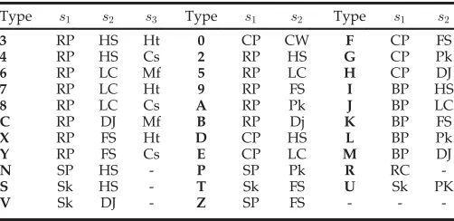
The USF dataset [5] is a large outdoor gait database, consisting of 122 subjects. A number of covariates are presented: camera view-points (left/right), shoes (type A/type B), surface types (grass/ concrete), carrying conditions (with/without a briefcase), elapsed time (May/Nov.), and clothing. Based on a gallery with 122 sub-jects, there are 12 pre-designed experiments for algorithm evalua-tion, which are summarized in Table 1. The second gait database, namely, the OU-ISIR-B dataset [16], was recently constructed for studying the effect of clothing. The evaluation set includes 48 sub-jects walking on a treadmill with up to 32 types of clothes combina-tions, as listed in Table 2. The gallery consists of the 48 subjects in standard clothes (i.e., type 9: regular pantsþfull shirt), whereas the probe set includes 856 gait sequences of the same 48 subjects in

the other 31 clothes types. Several images from the USF and OU-ISIR-B datasets are shown in Fig. 5. For both datasets, the gallery is used for training. In this work, we employ two templates sepa-rately, namely, GEI (with the default size 12888 pixels) and downsampled Gabor-filtered GEI (referred to as Gabor, with size 320352pixels).

We employ rank-1/rank-5 correct classification rate (CCR) to evaluate the performance. Considering the random nature of our method, the results of different runs may vary to some extent. We repeat all the experiments 10 times and report the statistics (mean, std, maxima and minima) in Tables 3 and 7 for both datasets. The small std values (listed in Tables 3 and 7) of the 10 runs indicate the stability of our method. Therefore, throughout the rest of the paper, we only report the mean values.

6.2 Parameter Settings and Time Complexity Analysis There are only three parameters in our method, namely, the dimen-sion of random subspaceN, the base classifier numberL, and the number of projection directionsM for LE1/LE2. As discussed in Section 2.2, we should setNto a small number for great generaliza-tion abilityPðNÞ. The classifier numberLshould be large, since our classifier ensemble solution is based onthe law of large numbers

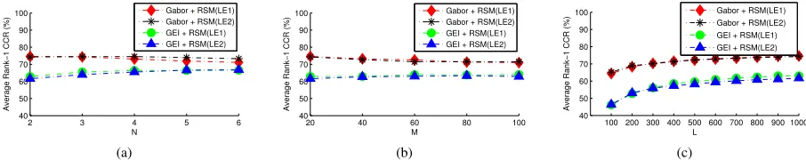
[27] (see Section 2.3). Like most subspace learning methods, the performance should not be sensitive to the number of projection directionsM for LE1/LE2 (unless it is extremely small). On the USF dataset (Exp. A-L) we check the average performance sensitiv-ity toN, M, andL, based on Gabor and GEI templates, respec-tively. By empirically settingL¼1;000 andM¼20, we run our methods withN set within the range½2;6. The results in Fig. 6a indicate that the performance is not sensitive to N. Based on L¼1;000, and N¼2, we conduct experiments with M¼ ½20; 40;60;80;100. The results in Fig. 6b suggest that the performance is stable forMwith different values. By settingN¼2andM¼20, we can also see from Fig. 6c that the performance is not decreasing with respect to the increasing number of classifiers. These observa-tions are consistent with our expectation that the performance is not sensitive to these three parameters. For the rest of this paper, we only report the results based onN¼2,M¼20andL¼1;000.

TABLE 1

Twelve Pre-Designed Experiments on the USF Dataset

Exp. A B C D E F

# Seq. 122 54 54 121 60 121 Covariates V H VH S SH SV

Exp. G H I J K L

# Seq. 60 120 60 120 33 33 Covariates SHV B BH BV THC STHC

Abbreviation note: V-View, H-Shoe, S-Surface, B-Briefcase, T-Time, C-Clothing.

TABLE 2

Different Clothing Combinations in the OU-ISIR-B Dataset

Type s1 s2 s3 Type s1 s2 Type s1 s2 3 RP HS Ht 0 CP CW F CP FS

4 RP HS Cs 2 RP HS G CP Pk

6 RP LC Mf 5 RP LC H CP DJ

7 RP LC Ht 9 RP FS I BP HS

8 RP LC Cs A RP Pk J BP LC

C RP DJ Mf B RP Dj K BP FS

X RP FS Ht D CP HS L BP Pk

Y RP FS Cs E CP LC M BP DJ

N SP HS - P SP Pk R RC

-S Sk HS - T Sk FS U Sk PK

V Sk DJ - Z SP FS - -

-Abbreviation note: RP - Regular pants, BP - Baggy pants, SP - Short pants, HS - Half shirt, FS - Full shirt, LC - Long coat, CW - Casual wear, RC - Rain coat, Ht - Hat, CP-Casual pants, Sk - Skirt, Pk - Parker, DJ - Down jacket, Cs - Casquette cap, Mf - Muffler,si-ithclothes slot.

We analyze the time complexity for training the L LE1/LE2-based classifiers. For a LE1-LE1/LE2-based classifier in Algorithm 1, it takes OðnNN2

1Þ(resp.OðcNN12Þ) forSwl (resp.Slb) andOðN13Þfor

eigen-value decomposition. N1 is the template’s row number (i.e.,

N1¼128for GEI,N1¼320for Gabor), whilenandcare the

num-ber of training samples and classes, respectively. Since, in our case, n > candn > N1, the time complexity for generatingLLE1-based

classifiers can be written asOðLnNN2

1Þ. For a LE2-based classifier

in Algorithm 2, it takesOðc2_{SÞfor the QR decomposition, where}

S¼NN1. CalculatingSlBandSWl requiresOðc3ÞandOðc2nÞ, while

calculatingZandY requiresOðnScÞandOðSc2_{Þ. Solving the}

eigen-value decomposition problem of ðSl WÞ

1_Sl

B takes Oðc3Þ and the

final solutionVl_{is obtained by matrix multiplication, which takes}

OðcSMÞ. Since in our casen > candS > c, the time complexity for generatingLLE2-based classifiers isOðLnScÞ, which can also be written asOðLnNN1cÞ. We run the matlab code of our method on a

PC with an Intel Core i5 3.10 GHz processor and 16GB RAM. For the USF dataset, we report the training/query time (with L¼1;000) in Table 4. Note the classifiers are trained in an offline manner and can be used to identify probe sets with various covari-ates. It is clear that LE2 is very efficient when the dimension is large. For example, based on Gabor templates, LE2 only takes about1=10of LE1’s training time.

6.3 Performance Gain Analysis and Algorithms Comparison

Based on GEI and Gabor templates, we evaluate the effect of sup-pressing the ratio of false votesPci¼11Vfalsei to true votesVtrue, as

defined in (10) by using LE and HDF. For a probe set withKgait

sequences, according to (10) we defineG^as

^

G¼median ( Pc1

i¼1V i false

Vtrueþ

)K

k¼1

; (17)

which is used to reflect the general ratio over the whole probe set. We set¼1to avoid the trivial results. Over the 12 probe sets (A-L) on the USF dataset, the distribution of^Gand the performance are reported in Fig. 7 and Table 5. We can observe that, LE1/LE2 can reduce^Gto some extent, and RSM(LE1)/RSM(LE2) is less sen-sitive to covariates such as viewpoint, shoe, and briefcase (A-C, H-J). On the other hand, RSM-HDF can significantly suppressG^and yields competitive accuracies in tackling the hard problems caused by walking surface and elapsed time (D-G, K-L).

On the USF dataset, we also compare our method Gabor+RSM-HDF with the recently published works, with the rank-1/rank-5 CCRs reported in Table 6. These works include Baseline [5], hidden Markov models (HMM) [31], GEI+Fusion [4], CSA+DATER [8], DNGR [13], matrix-based marginal Fisher analysis (MMFA) [21], GTDA [9], linearization of DLLE (DLLE/L) [7], TRIMAP [10], Image-to-Class [11], Gabor-PDF+LGSR [12], CGI+Fusion [14], sparse reconstruction based metric learning (SRML) [23], and sparse bilinear discriminant analysis (SBDA) [22]. From Table 6, we can see that in terms of rank-1 CCRs, our method outperforms other algorithms on all the 12 probe sets. Our method has an aver-age rank-1 CCR more than 10 percent higher than the second best method (i.e., Gabor-PDF+LGSR [12]), and also the highest average rank-5 CCR. It is significantly superior than others on the challeng-ing tasks D-G, and K-L, which are under the influences of walkchalleng-ing surface, elapsed time and the combination of other covariates. Although these walking conditions may significantly corrupt the gait features, our proposed HDF scheme (based on LE1 and LE2) can still suppressGof (10), leading to competitive accuracies. We

Fig. 6. On the performance sensitivity to the parameters on the USF dataset: (a)Nis the dimension of the random subspace; (b)Mis the number of projection directions of LE1/LE2; (c)Lis the classifier number.

TABLE 4

Running Time (Seconds) on the USF Dataset

- Training Time Query Time Per Seq. GEIþRSM(LE1) 91.42 0.58 GEIþRSM(LE2) 28.66 0.26 GaborþRSM(LE1) 320.09 0.60 GaborþRSM(LE2) 32.79 0.31

TABLE 3

Performance Statistics in Terms of Rank-1 CCRs (Percent) for 10 Runs on the USF Dataset

- maxima minima std mean GEI + RSM 52.44 50.73 0.62 51.45 GEI + RSM(LE1) 64.08 62.36 0.49 63.01 GEI + RSM(LE2) 62.79 59.81 0.91 61.72 GEI + RSM-HDF 70.90 69.20 0.50 70.01 Gabor + RSM 67.58 66.30 0.46 67.06 Gabor + RSM(LE1) 75.29 73.89 0.49 74.56 Gabor + RSM(LE2) 74.95 73.45 0.36 74.27 Gabor + RSM-HDF 82.12 80.30 0.53 81.17

notice that our method only has 42 percent rank-1 CCRs for probe sets K-L. In these cases, elapsed time is coupled with other covari-ates like walking surface, clothing, and shoe, as listed in Table 1. These walking conditions may significantly increase the number of irrelevant featuresm, which would result in a lowerPðNÞin (6). According to Section 2.3, a lowerPðNÞwould lead to a higherGin (10), which contributes negatively to the performance. Neverthe-less, experimental results suggest our method is robust to most covariates in the outdoor environment.

6.4 In Tackling the Clothing Challenges

Clothing was deemed as the most challenging covariate [15], and there are only a few works that have studied the effect of various clothes types. Recently, Hossain et al. built the OU-ISIR-B dataset [16] with 32 combinations of clothes types, as shown Table 2. Based on an additional training set that covers all the possible clothes types, they proposed an adaptive part-based method [16] for cloth-ing-invariant gait recognition. On this dataset, based on Gabor tem-plates, we evaluate our methods RSM(LE1), RSM(LE2) and RSM-HDF. The statistics of our methods over 10 runs are reported in

Table 7. Compared with the part-based method [16], Gabor+RSM-HDF can yield a much higher accuracy, as shown in Table 8. It is worth noting that different from [16], our method does not require the training set that covers all the possible clothes types and can generalize well to unseen clothes types.

We also study the effect of different clothes types, and the rank-1 CCRs for 3rank-1 probe clothes types are reported in Fig. 8. For most of the clothes types, our method can achieve more than 90 percent rank-1 accuracies. However, the performance can be affected with several clothes types that cover large parts of the human body. In this case, a large number of irrelevant featuresmwould result in

TABLE 5

Rank-1 CCRs (Percent) of Our Methods on the USF Dataset

Exp. A B C D E F G H I J K L Avg.

GEI + RSM 89 93 82 24 27 16 16 83 69 54 18 9 51.36 GEI + RSM(LE1) 95 94 86 42 50 23 35 88 88 72 26 19 62.88 GEI + RSM(LE2) 96 94 82 40 46 27 29 87 83 72 19 18 61.70 GEI + RSM-HDF 98 95 88 54 60 37 44 90 93 83 33 21 70.16 Gabor + RSM 96 94 87 47 45 24 38 96 97 85 25 27 67.13 Gabor + RSM(LE1) 100 95 93 62 63 42 50 97 96 89 23 29 74.65 Gabor + RSM(LE2) 98 94 93 60 58 39 47 97 97 92 34 31 74.09 Gabor + RSM-HDF 100 95 94 73 73 55 64 97 99 94 42 42 81.15

TABLE 6

Algorithms Comparison in Terms of Rank-1/Rank-5 CCRs (Percent) on the USF Dataset

Exp. A B C D E F G H I J K L Avg.

Rank-1 CCRs

Baseline[5] 73 78 48 32 22 17 17 61 57 36 3 3 40.96 HMM [31] 89 88 68 35 28 15 21 85 80 58 17 15 53.54 GEI + Fusion [4] 90 91 81 56 64 25 36 64 60 60 6 15 57.66 CSA + DATER [8] 89 93 80 44 45 25 33 80 79 60 18 21 58.51 DNGR [13] 85 89 72 57 66 46 41 83 79 52 15 24 62.81 MMFA [21] 89 94 80 44 47 25 33 85 83 60 27 21 59.90 GTDA [9] 91 93 86 32 47 21 32 95 90 68 16 19 60.58 DLLE/L [7] 90 89 81 40 50 27 26 65 67 57 12 18 51.83 TRIMAP [10] 92 94 86 44 52 27 33 78 74 65 21 15 59.66 Image-to-Class [11] 93 89 81 54 52 32 34 81 78 62 12 9 61.19 Gabor-PDF + LGSR [12] 95 93 89 62 62 39 38 94 91 78 21 21 70.07 CGI + Fusion [14] 91 93 78 51 53 35 38 84 78 64 3 9 61.69 SRML [23] 93 94 85 52 52 37 40 86 85 68 18 15 66.50 SBDA [22] 93 94 85 51 50 29 36 85 83 68 18 24 61.35 Gabor + RSM-HDF (Ours) 100 95 94 73 73 55 64 97 99 94 42 42 81.15

Rank-5 CCRs

Baseline [5] 88 93 78 66 55 42 38 85 78 62 12 15 64.54 GEI + Fusion [4] 94 94 93 78 81 56 53 90 83 82 27 21 76.23 CSA + DATER [8] 96 96 94 74 79 53 57 93 91 83 40 36 77.86 DNGR [13] 96 94 89 85 81 68 69 96 95 79 46 39 82.05 MMFA [21] 98 98 94 76 76 57 60 95 93 84 48 39 79.90 GTDA [9] 98 99 97 68 68 50 56 95 99 84 40 40 77.58 DLLE/L[7] 95 96 93 74 78 50 53 90 90 83 33 27 71.83 TRIMAP [10] 96 99 95 75 72 54 58 93 88 85 43 36 77.75 Image-to-Class [11] 97 98 93 81 74 59 55 94 95 83 30 33 79.17 Gabor-PDF + LGSR [12] 99 94 96 89 91 64 64 99 98 92 39 45 85.31 CGI + Fusion [14] 97 96 94 77 77 56 58 98 97 86 27 24 79.12 SBDA [22] 98 98 94 74 79 57 60 95 95 84 40 40 79.93 Gabor + RSM-HDF (Ours) 100 98 98 85 84 73 79 98 99 98 55 58 88.59

TABLE 7

Performance Statistics in Terms of Rank-1 CCRs (Percent) for 10 Runs on the OU-ISIR-B Dataset

a higherGin (10), which would hamper the performance (as dis-cussed in Section 6.3). Specifically, the results are less satisfactory when the following 3 clothes types are encountered: 1) clothes type R, (i.e., raincoat) with a rank-1 CCR of 63.3 percent; 2) clothes type H, (i.e., casual pants + down jacket) with a rank-1 CCR of 52.1 per-cent; 3) clothes type V, (i.e., skirt + down jacket) with a rank-1 CCR of 52.2 percent. Nevertheless, in general the results suggest that our method is robust to clothing.

7

CONCLUSION

In this paper, we model the effect of covariates as a partial feature corruption problem with unknown locations and propose a RSM-based classifier ensemble solution. The theoretical basis suggests that its insensitivity to a large number of covariates in ideal cases. To tackle the hard problems in real cases, we then propose two strategies, i.e., LE and HDF, to suppress the ratio of false votes to true votes before the majority voting. Experimental results suggest that our method is less sensitive to the most challenging covariates like clothing, walking surface, and elapsed time. Our method has only three parameters, to which the performance is not sensitive. It can be trained within minutes and perform real-time recognition in less than 1 second, which suggests that it is practical in real-world applications.

ACKNOWLEDGMENTS

The authors would like to thank the support from the Royal Society’s International Exchange Programme (IE120092) and the constructive comments from the anonymous reviewers.

REFERENCES

[1] P. K. Larsen, E. B. Simonsen, and N. Lynnerup, “Gait analysis in forensic medicine,”J. Forensic Sci., vol. 53, pp. 1149–1153, 2008.

[2] I. Bouchrika, M. Goffredo, J. Carter, and M. S. Nixon, “On using gait in forensic biometrics,”J. Forensic Sci, vol. 56, no. 4, pp. 882–889, 2011. [3] D. Cunado, M. S. Nixon, and J. Carter, “Automatic extraction and

descrip-tion of human gait models for recognidescrip-tion purposes,”Comput. Vis. Image Understanding, vol. 90, no. 1, pp. 1–41, 2003.

[4] J. Han and B. Bhanu, “Individual recognition using gait energy image,” IEEE Trans. Pattern Anal. Mach. Intell., vol. 28, no. 2, pp. 316–322, Feb. 2006. [5] S. Sarkar, P. J. Phillips, Z. Liu, I. R. Vega, P. Grother, and K. W. Bowyer,

“The humanID gait challenge problem: Data sets, performance, and analy-sis,”IEEE Trans. Pattern Anal. Mach. Intell., vol. 27, no. 2, pp. 162–177, Feb. 2005.

[6] H. Iwama, M. Okumura, Y. Makihara, and Y. Yagi, “The OU-ISIR gait data-base comprising the large population dataset and performance evaluation of gait recognition,”IEEE Trans. Inf. Forensics Security, vol. 7, no. 5, pp. 1511–1521, Oct. 2012.

[7] X. Li, S. Lin, S. Yan, and D. Xu, ”Discriminant locally linear embedding with high-order tensor data,”IEEE Trans. Syst. Man Cybern B, vol. 38, no. 2, pp. 342–352, Apr. 2008.

[8] D. Xu, S. Yan, D. Tao, L. Zhang, X. Li, and H. J. Zhang, ”Human gait recog-nition with matrix representation,”IEEE Trans. Circuits Syst. Video Technol., vol. 16, no. 7, pp. 896–903, Jul. 2006.

[9] D. Tao, X. Li, X. Wu, and S. J. Maybank, ”General tensor discriminant anal-ysis and gabor features for gait recognition,” IEEE Trans. Pattern Anal. Mach. Intell., vol. 29, no. 10, pp. 1700–1715, Oct. 2007.

[10] C. Chen, J. Zhang, and R. Fleischer, ”Distance approximating dimension reduction of Riemannian manifolds,”IEEE Trans. Syst. Man Cybern. B, vol. 40, no. 1, pp. 208–217, Feb. 2010.

[11] Y. Huang, D. Xu, and T. Cham, ”Face and human gait recognition using image-to-class distance,”IEEE Trans. Circuits Syst. Video Technol., vol. 20, no. 3, pp. 431–438, Mar. 2010.

[12] D. Xu, Y. Huang, Z. Zeng, and X. Xu, ”Human gait recognition using patch distribution feature and locality-constrained group sparse representation,” IEEE Trans. Image Process., vol. 21, no. 1, pp. 316–326, Jan. 2012.

[13] Z. Liu and S. Sarkar, ”Improved gait recognition by gait dynamics normal-ization,”IEEE Trans. Pattern Anal. Mach. Intell., vol. 28, no. 6, pp. 863–876, Jun. 2006.

[14] C. Wang, J. Zhang, L. Wang, J. Pu, and X. Yuan, ”Human identification using temporal information preserving gait template,”IEEE Trans. Pattern Anal. Mach. Intell., vol. 34, no. 11, pp. 2164–2176, Nov. 2012.

[15] D. Matovski, M. S. Nixon, S. Mahmoodi, and J. Carter, ”The effect of time on gait recognition performance,”IEEE Trans. Inf. Forensics Security, vol. 7, no. 2, pp. 543–552, Apr. 2012.

[16] M. A. Hossain, Y. Makihara, J. Wang, and Y. Yagi, ” Clothing-invariant gait identification using part-based clothing categorization and adaptive weight control,”Pattern Recognit., vol. 43, no. 6, pp. 2281–2291, 2010.

[17] T. K. Ho, ”The random subspace method for constructing decision forests,” IEEE Trans. Pattern Anal. Mach. Intell., vol. 20, no. 8, pp. 832–844, Aug. 1998. [18] X. Wang and X. Tang, ”Random sampling for subspace face recognition,”

Int. J. Comput. Vis., vol. 70, no. 1, pp. 91–104, 2006.

[19] Y. Guan, C.-T. Li, and Y. Hu, ” Random subspace method for gait recog-nition,” inProc. IEEE Int. Conf. Multimedia Expo Workshops, 2012, pp. 284–289. [20] Y. Guan, C.-T. Li, and Y. Hu, ”Robust clothing-invariant gait recognition,” inProc. 8th Int. Conf. Intell. Inf. Hiding Multimedia Signal Process., 2012, pp. 321–324.

[21] D. Xu, S. Yan, D. Tao, S. Lin, and H. Zhang, ”Marginal Fisher analysis and its variants for human gait recognition and content-based image retrieval,” IEEE Trans Image Process., vol. 16, no. 11, pp. 2811–2821, Nov. 2007. [22] Z. Lai, Y. Xu, Z. Jin, and D. Zhang, ”Human gait recognition via sparse

dis-criminant projection learning,”IEEE Trans. Circuits Syst. Video Technol., vol. 24, no. 10, pp. 1651–1662, Oct. 2014.

[23] J. Lu, G. Wang, and P. Moulin, ”Human identity and gender recognition from gait sequences with arbitrary walking directions,”IEEE Trans. Inf. For-ensics Security, vol. 9, no. 1, pp. 51–61, Jan. 2014.

[24] J. Yang, D. Zhang, A. F. Frangi, and J. Yang, ”Two-dimensional PCA: A new approach to appearance-based face representation and recognition,” IEEE Trans. Pattern Anal. Mach. Intell., vol. 26, no. 1, pp. 131–137, Jan. 2004. [25] C. Walck,Handbook on Statistical Distributions for Experimentalists.

Stock-holm, Sweden: Univ. Stockholm Press, 2007.

[26] J. Kittler, M. Hatef, R. P. W. Duin, and J. Matas, ”On combining classifiers,” IEEE Trans. Pattern Anal. Mach. Intell., vol. 20, no. 3, pp. 226–239, Mar. 1998. [27] C. M. Grinstead and J. L. Snell,Introduction to Probability.Providence, RI,

USA: Amer. Math. Soc., 1997.

[28] M. Li and B. Yuan, ”2D-LDA: A statistical linear discriminant analysis for image matrix,”Pattern Recognit. Lett., vol. 26, pp. 527–532, 2005.

[29] J. Ye, Q. Li, H. Xiong, H. Park, R. Janardan, and V. Kumar, ”IDR/QR: An incremental dimension reduction algorithm via QR decomposition,”IEEE Trans. Knowl. Data Eng., vol. 17, no. 9, pp. 1208–1222, Sep. 2005.

[30] L. N. Trefethen, and D. Bau,Numerical Linear Algebra.Philadelphia. PA, USA: SIAM, 1997.

[31] A. Kale, A. Sundaresan, A. N. Rajagopalan, N. P. Cuntoor, A. K. Roy-Chowdhury, V. Kruger, and R. Chellappa, ”Identification of humans using gait,”IEEE Trans. Image Process., vol. 13, no. 9, pp. 1163–1173, Sep. 2004.

TABLE 8

Algorithms Comparison in Terms of Rank-1 CCRs (Percent) on the OU-ISIR-B Dataset

Part-based method [16] GaborþRSM-HDF (Ours)

63.9 90.7