http://wrap.warwick.ac.uk
Original citation:
Chen, Yunfei, Sabnis-Thomas, Kalen and Abd-alhameed, Raed. (2016) New formula for
conversion efficiency of RF EH and its wireless applications. IEEE Transactions on
Vehicular Technology. doi : 10.1109/TVT.2016.2515843
Permanent WRAP url:
http://wrap.warwick.ac.uk/77006
Copyright and reuse:
The Warwick Research Archive Portal (WRAP) makes this work by researchers of the
University of Warwick available open access under the following conditions. Copyright ©
and all moral rights to the version of the paper presented here belong to the individual
author(s) and/or other copyright owners. To the extent reasonable and practicable the
material made available in WRAP has been checked for eligibility before being made
available.
Copies of full items can be used for personal research or study, educational, or not-for
profit purposes without prior permission or charge. Provided that the authors, title and
full bibliographic details are credited, a hyperlink and/or URL is given for the original
metadata page and the content is not changed in any way.
Publisher’s statement:
“© 2016 IEEE. Personal use of this material is permitted. Permission from IEEE must be
obtained for all other uses, in any current or future media, including reprinting
/republishing this material for advertising or promotional purposes, creating new
collective works, for resale or redistribution to servers or lists, or reuse of any
copyrighted component of this work in other works.”
A note on versions:
The version presented here may differ from the published version or, version of record, if
you wish to cite this item you are advised to consult the publisher’s version. Please see
the ‘permanent WRAP url’ above for details on accessing the published version and note
that access may require a subscription.
New Formula for Conversion Efficiency of RF EH
and its Wireless Applications
Yunfei Chen, Senior Member, IEEE, Kalen T. Sabnis, Raed A. Abd-Alhameed
Abstract— Existing works on energy harvesting wireless
sys-tems often assume a constant conversion efficiency for the energy harvester. In practice, the conversion efficiency often varies with the input power. In this work, based on a review of existing energy harvesters in the literature, a heuristic expression for the conversion efficiency as a function of the input power is derived by curve fitting. Using this function, two example energy harvesters are used to analyze the realistic performances of wireless relaying and wireless energy transfer. Numerical results show that the realistic performances of the wireless systems could be considerably different from what predicted by the existing analysis.
Index Terms— Energy harvesting, relaying, throughput,
wire-less energy transfer.
I. INTRODUCTION
Energy efficiency is a long-standing problem in wireless communications [1], [2]. One of the most promising solutions is radio frequency (RF) energy harvesting (EH) [3]. The most important performance measure of the RF energy harvester is perhaps the conversion efficiency, defined as the ratio of the output power to the input power of the energy harvester. There have been quite a few different designs of RF energy harvester in the literature, such as [4] - [16], among others. A detailed discussion of these works will be presented in the next section, based on which a heuristic formula of the conversion efficiency will be obtained. In these designs, a common conclusion is that the conversion efficiency depends on the input power.
On the other hand, many researchers have studied the use of energy harvesting in wireless systems. For example, in [17], an energy-constrained wireless link was studied, where the receiver relies on harvesting the energy from the transmitter, by maximizing the throughput. In [18], an energy harvesting relaying system was studied. Two energy harvesting methods, time-switching (TS) and power-splitting (PS), were proposed. In all these works and most existing works, it was assumed that the conversion efficiency of the energy harvester is a fixed value that does not depend on the input power. However, this is not the case in reality. Thus, it is of great interest to study the realistic performances of the wireless systems by treating the conversion efficiency of the energy harvester as a function of the input power, as in practice.
In this paper, we study the realistic performances of the wireless systems under the assumption that the conversion efficiency of the energy harvester is a function of the input
Yunfei Chen and Kalen Thomas Sabnis are with the School of Engi-neering, University of Warwick, Coventry, U.K. CV4 7AL (e-mail: [email protected], [email protected])
Raed A. Abd-Alhameed is with the School of Engineering and In-formatics, Bradford University, Bradford, U.K. BD7 1 DP (e-mail: [email protected]).
power. To do this, we first derive a heuristic model for the conversion efficiency as a function of the input power. Using this, the realistic throughputs of relaying in [18] and wireless energy transfer in [17] are analyzed. Numerical results show that the realistic throughput depends on the specific energy harvesters considered, and it varies significantly when the conversion efficiency changes.
This work aims to find a more practical expression for the efficiency of existing harvesters and use it to evaluate the realistic performances of systems using existing harvesters. It focuses on the theoretical aspect of existing harvesters. To the best of the authors’ knowledge, this has not be done before and thus, it represents contribution. To do this, it may be sufficient to use data from existing experiments in trusted sources. However, designing a new harvester or performing new experiments to collect new data could be an interesting future work when relevant laboratory resources are available.
II. RELATED WORK ONRFENERGY HARVESTER
This section does not aim to provide a complete review of all works on RF energy harvester designs due to limited space. For such a review, the readers are referred to the survey in [19]. Rather, this section aims to provide a discussion of some representative works, based on which a heuristic model of the conversion efficiency can be derived. Thus, we focus on [4] - [16].
A. Low Input Power
It is desirable to have a RF energy harvester that can operate over a long distance at a low input power with high sensitivity. Reference [4] designed a RF energy harvester with a high sensitivity of -26.3 dBm. It works at a frequency of 868
M Hz with a long distance of 25 meters, when the source transmits at 1.78 W. In this case, the peak efficiency of this harvester is 22 %. In [5], further improvements were made. In particular, the sensitivity was increased to -27dBmand hence the range was increased to 27 meters. The peak efficiency became 36%. Reference [6] designed a fully passive RFID tag with a sensitivity of -12dBm. Further, the peak efficiency of the harvester implemented in this tag is 37%. In [7], a 953
M Hz rectenna was designed. It allows a peak efficiency of 29% achieved at -9.9dBm.
mW
1.3 mW. Further improvements were done in [9], where a peak efficiency of 60% with a sensitivity of -21 dBm was achieved at 868 M Hz. The efficiency is above 30 % when the input power is between 0.05 mW and 1.5 mW. Such a wide range of input power is very useful, as the input power in practice is often unpredictable. Reference [10] designed a dual-band harvester at the GSM1800 band and 3G band to harvest energies from multiple bands. Tests showed that it has a peak efficiency of 51%, and its normal operating efficiency is between 16% and 43%. In [11], a 906M Hzenergy harvester was designed with a peak efficiency of 60% and a sensitivity of -22.5dBm. It can operate at a distance of 42 meters from a 4 W power source. In [12], another GSM band harvester was designed that can achieve a peak efficiency of 67.5% using a differential drive technology. Further tests also showed that this harvester could be used for 500M Hz DTV band to achieve a peak efficiency of 80%.
All the above designs operate at low input power and are suitable for long-range harvesting applications. Their peak efficiencies are normally achieved at less than 0.2mW.
B. High Input Power
In this subsection, several designs operate at high input power are discussed. Their peak efficiencies are achieved at more than 0.2mW.
Reference [13] designed a 2.4 GHz energy harvester with a peak efficiency of 22.7% achieved at 0.5dBmand a sensitivity of -10 dBm. In [14], another energy harvester at a frequency of 868 M Hz was designed for RFID and remote powering applications. This design aimed to maximize the range of the input power that provides high efficiency, in particular, an efficiency higher than 40% for a range of 14dB input power. This design has a peak efficiency of 60% achieved at 0.5mW. Reference [15] proposed a dual-rectifier energy harvester such that the overall range of input power with high efficiency was considerably increased. The harvester can achieve an efficiency above 30% for up to 30 mW. It was tuned to 915M Hzbut can be modified to other frequencies too. It achieves a peak efficiency of 72 % at an input of 4 mW. Finally, in [16], a RF energy harvester operating at 2.45 GHz was designed. It can achieve an efficiency above 30% for up to 4 mW. Its peak efficiency of 70% can be obtained at an input power of 1 mW.
Table I shows the main parameters of the energy harvesters discussed above, where fc is the operating frequency, ηmax
is the maximum achievable efficiency, Pin is the input power
that achieves ηmaxandǫ is the sensitivity.
C. Heuristic Model
The above papers have motivated us to obtain a heuristic model for the conversion efficiency as a function of the input power. After testing several different nonlinear functions in curve fitting, we conclude that the following rational function fits all the curves best using a minimum root mean squared error criterion as
η[x] = p2x
2+p 1x+p0
q3x3+q2x2+q1x+q0
(1)
MAIN PARAMETERS OF DIFFERENT ENERGY HARVESTERS.
Ref. fc
(MHz) ηmax Pin
(mW) ǫ
(dBm) Fabrication [4] 868 22% 0.015 -26.3 90 nm CMOS
[5] 868 36% 0.018 -27 90 nm CMOS
[6] 900 37% 0.16 -12 130 nm CMOS
[7] 953 29% 0.1 unknown 350 nm CMOS
[8] 928 45% 0.16 -14 130 nm CMOS
[9] 868 60% 0.15 -21 130 nm CMOS
[10] 1800
2200 51% 0.16 unknown substrateǫr= 2.33 [11] 906 60% 0.16 -22.6 250 nm CMOS [12] 953 68% 0.06 unknown 180 nm CMOS
[13] 2400 23% 0.5 -10 130 nm CMOS
[14] 868 58% 0.5 -17 130 nm CMOS
[15] 915 72% 4 unknown substrateǫr= 4.0
[16] 2450 70% 1 unknown substrateǫr= 3.55
where x is the input power with a unit of mW, η
is the efficiency as a percentage and the parameters of
p0, p1, p2, q0, q1, q2, q3 are different for different harvesters.
This is achieved by testing the order of numerator from 0 to 5 and the order of denominator from 1 to 5 for the rational function in MATLAB curve-fitting and choosing the orders for best tradeoff between accuracy and complexity. All these observations are made heuristically from existing experiments without any systematic analysis, as it is impossible to perform such an analysis for these complicated circuits. However, we have done this for 36 different harvesters, almost all existing harvesters in the literature, and they all follow this model. Thus, (1) does have generality. Moreover, it is true that curve-fitting is limited by the range considered. However, most existing harvesters operate with an input power below 4 mW. In this case, our curve-fitting is useful for this small but practical range between 0 and 4 mW. Some insights can also be gained from (1). For example, when the input power x
is small, the efficiency is mainly determined byp0/q0. Also,
when the input power x is large, the efficiency decreases at a rate 1/x but is also determined by p2/q3. Figs. 1 and 2
compare the curve fitting results with the experimental results for the harvesters provided in [11] and [4], respectively. We did not reproduce the experimental results but only took them from the figures provided in the papers. One sees that they agree with each other reasonably well. Table II gives the fitting parameters for all the energy harvesters discussed above. The value of q3 is normalized to 1 and therefore is not listed in
Table II.
III. WIRELESSAPPLICATIONS
0 0.1 0.2 0.3 0.4 0.5 0.6 0.7 0.8 0.9 1 20
25 30 35 40 45 50 55 60
Input Power (mw)
Efficiency (%)
[image:4.595.88.263.56.197.2]Experimental Curve fitting
Fig. 1. Comparison of the fitted curve and the experimental curve for [11].
0 0.02 0.04 0.06 0.08 0.1 0.12 0.14 0.16
0 5 10 15 20 25
Input Power (mw)
Efficiency (%)
Experimental Curve fitting
Fig. 2. Comparison of the fitted curve and the experimental curve for [4].
A. Wireless relaying application
We consider the same system as [18] but with varying efficiency. In this case, a three-node relaying system is used, where the source sends information and energy to the relay and the relay uses the harvested energy to forward the information to the destination. There is no direct link. Each node has a single antenna and operates in half-duplex. The source-to-relay and relay-to-destination links are orthogonal in time. Assume that the total communication time is T.
In TS, a faction of the total time αT is used for energy harvesting at the relay, followed by(1−α)T
2 for information
reception at the relay and(1−α)T
2 for information reception
at the destination, whereαis the TS coefficient. In the existing analysis, η is assumed constant and independent of the input power. Thus, one has Eh = ηPs|h|2αT as the harvested
energy, where Ps is the source transmission power and h is
the complex channel gain of the source-to-relay link. In this work and in reality, η is a function of the input power. By replacingη with (1) and following a similar analysis to [18], the outage probabilities can be derived as (2) for variable-gain relaying and (3) for fixed-variable-gain relaying in the next page, where γ0= 2R−1is the threshold SNR for outage,R is the
constant throughput required by the source, Γ1 = PsE{|h|
2 }
σ2
ra+σ2rc ,
TABLE II
FITTING PARAMETERS OF DIFFERENT ENERGY HARVESTERS.
Ref. p2 p1 p0 q2 q1 q0
[4] 1.34 5.2e-5 1.61e-6 0.0547 -0.000318 2.87e-6 [5] -5.15e5 1.16e5 -125 5.35e4 939 16.1 [6] 1.23 10.5 -0.238 -0.125 0.24 0.00045 [7] 14.1 0.171 -0.00284 0.956 -0.119 0.0069 [8] 108 1.47 -0.11 2.35 -0.0652 0.00923 [9] 85.3 19.4 -0.15 1.28 0.315 0.00023 [10] 4.52e5 7.59e5 685 1.11e4 1.43e4 73.1 [11] 78.5 -2.34 1.62 2.43 -0.482 0.0658
[12] 413 1160 704 15.1 25.4 12.5
[13] 230 -20.5 0.623 9.24 -0.77 0.0808 [14] 300 -12.7 0.135 4.4 -0.0104 -0.00166
[15] 0 7.30e4 394 -3.32 951 98
[16] 99.9 140 -0.059 -0.295 2.71 0.093
Γ2= E{|g|
2}
σ2
da+σ
2
dc
,gis the complex channel gain of the relay-to-destination link,σ2
ra andσ
2
rc are the variances of the noise at
the relay from the RF antenna and RF-baseband conversion, respectively,σ2
daandσ
2
dcare the variances of the noise at the
destination from the RF antenna and RF-baseband conversion, respectively.
Finally, the throughput in this case is given by [18]
βT SV GN ew =
R
2(1−α)(1−P
N ew
out−T SV G) (4)
βT SF GN ew =
R
2(1−α)(1−P
N ew
out−T SF G). (5)
If PS is used, a fraction of the received signal is harvested without any dedicated harvesting time. In this case, the trans-mission from the source to the relay takes T2 seconds for both harvesting and reception and the relay takes another T2 seconds to use the harvested energy to transmit the signal to the destination. Using the varying efficiency in (1) and following a similar analysis to [18], the outage probabilities are (6) for variable-gain relaying and (7) for fixed-gain relaying in the next page, whereΓ′
1=
PsE{|h|2}
σ2
ra+ σ2
rc
1−ρ .
Then, the throughput is given by [18]
βP SV GN ew =
R 2(1−P
N ew
out−P SV G) (8)
βN ewP SF G=
R 2(1−P
N ew
out−P SF G). (9)
Note that the results for fixed-gain relaying are new, as [18] did not consider fixed-gain.
B. Wireless energy transfer
In [17], the authors proposed a wireless energy transfer network. Using the same system model, we consider a network where the access point transmits energy to the nodes in the downlink for τ0T seconds, and then the nodes use the
harvested energy to transmit information to the access point in the uplink for τ1T seconds, τ2T seconds, and so on, in
a time division multiple access (TDMA) way, whereT is the total transmission time andPiτi = 1. In the existing analysis,
one has Ei = ηPAhiτ0T as the harvested energy, where η
is the constant conversion efficiency assumed in [17], PA is
[image:4.595.310.568.64.207.2]PoutN ew−T SV G= 1− Γ
1 0
e Γ1 Γ2(2α)η[(t+γ0)(σ2
ra+σ2rc)](t+γ0 )(σ2
ra+σ2rc)tdt (2)
PN ew
out−T SF G= 1−
e−γΓ10
Γ1 Z ∞
0
e− t
Γ1−
γ0 (1−α)(Γ1+1)
Γ2(2α)η[(t+γ0)(σ2
ra+σ2rc)](t+γ0 )(σ2
ra+σ2rc)tdt (3)
PN ew
out−P SV G= 1−
e− γ0 Γ′
1
Γ′
1 Z ∞
0
e − t
Γ′
1
− γ0 (t+γ0 +1)
Γ2η[ρ(t+γ0 )(σ2ra+σ 2
rc
1−ρ)]ρ(t+γ0)(σra2 +σ 2
rc
1−ρ)tdt (6)
PoutN ew−P SF G= 1−
e− γ0 Γ′
1
Γ′
1 Z ∞
0
e − t
Γ′
1−
γ0 (Γ′1+1)
Γ2η[ρ(t+γ0)(σra2 +σ2rc
1−ρ)]ρ(t+γ0 )(σ2ra+σrc2
1−ρ)tdt (7)
power in the downlink from the access point to the node i,
τ0T is the harvesting time. In this work and in practice, the
conversion efficiency is a function of the input power such that
Ei =η[PAhi]PAhiτ0T, where (1) has been used. Following
a similar analysis to [17] but using a varying efficiency, the average throughput becomes
¯ Ri=−
τi
Γ ln 2
Z ∞
0
e−yΓ+
σ2τi
Γτ0η[PAy]PAyE
i(−
σ2
τi
Γτ0η[PAy]PAy
)dy
(10) whereσ2 is the variance of the additive white Gaussian noise,
Γis the average fading power,Ei(·)is the exponential integral
defined in [20, eq. (8.211)] and the relationship in [20, eq. (4.337.2)] has been used.
IV. NUMERICALRESULTS ANDDISCUSSION
In this section, numerical examples are presented to show the performances of the wireless systems examined using the realistic assumption that the conversion efficiency is dependent of the input power. To do this, we set Ps = 1, R = 3,
E{|h|2} =E{|g|2} = 1 andσ2
ra =σ
2
rc =σ
2
da =σ
2
dc =σ
2
in the wireless relaying in [18], PA = 1, Γ = 1, fmT = 1
in the wireless energy transfer in [17]. Also, for the existing analysis using constant conversion efficiency, we setη= 0.5. For our new analysis using varying conversion efficiency, we use the harvesters in [4] and [11]. Other constants and other harvesters can be examined in a similar way.
Fig. 3 shows the throughput for AF relaying using TS. Several observations can be made. First, there exists a max-imum throughput in all the curves shown. However, the optimal TS coefficient is considerably different for different curves. This means that one cannot use the performances predicted by the analysis based on the assumption of constant conversion efficiency to set up the optimal TS coefficient in practice. This must be done by using the realistic assumption of varying conversion efficiency. Second, fixed-gain relaying and variable-gain relaying have different performances. In particular, from Fig. 3, the maximum throughput for fixed-gain relaying is smaller than that for variable-gain relaying. Third, the harvester in [4] has a peak efficiency of 22%. Thus, the curves using [4] have a very small throughput and therefore require a larger value of the optimal TS coefficient in order to harvest more energies. In all the considered cases, the constant
α
0 0.1 0.2 0.3 0.4 0.5 0.6 0.7 0.8 0.9 1
Throughput (bits/s/Hz)
0 0.05 0.1 0.15 0.2 0.25 0.3 0.35 0.4 0.45 0.5
Constant η, fixed-gain Constant η, variable-gain
η using [11], fixed-gain
η using [11], variable-gain
η using [4], fixed-gain
[image:5.595.53.537.55.214.2]η using [4], variable-gain
Fig. 3. Throughput vs. αusing AF relaying and TS when
σ2
= 0.01.
ρ
0 0.1 0.2 0.3 0.4 0.5 0.6 0.7 0.8 0.9 1
Throughput (bits/s/Hz)
0 0.1 0.2 0.3 0.4 0.5 0.6
Constant η, fixed-gain
Constant η, variable-gain
η using [11], fixed-gain
η using [11], variable-gain
η using [4], fixed-gain
[image:5.595.328.555.81.377.2]η using [4], variable-gain
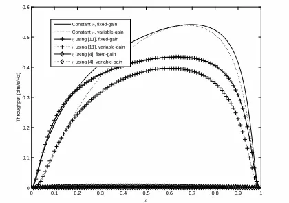
Fig. 4. Throughput vs. ρ using AF relaying and PS when
σ2= 0.01.
conversion efficiency has larger throughput or overestimates the realistic throughput.
[image:5.595.337.547.430.578.2]τ1
0.1 0.2 0.3 0.4 0.5 0.6 0.7 0.8 0.9
Throughput (bits/s/Hz)
0 0.5 1 1.5 2 2.5
Constant η
η using [11]
η using [4]
Fig. 5. Throughput vs.τ1with independent links whenσ2=
0.01.
curves for [4] and [11] still have smaller maximum throughput and smaller optimal PS factor than those for the constant conversion efficiency.
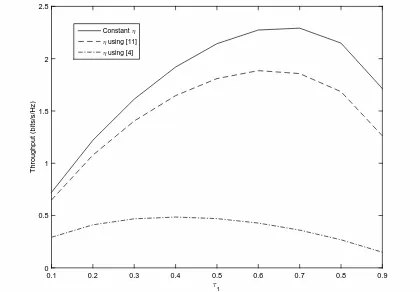
Fig. 5 shows the average throughput for wireless energy transfer in [17]. Only one node is considered such that τ0=
1−τ1, whereτ1 is the transmission time of node 1. One sees
that a maximum throughput exists in all curves, implying that it is necessary to choose the optimal value of the transmission time to achieve the highest throughput. Comparing the curve using the constant conversion efficiency with those using [11] and [4], one sees that they are significantly different. More specifically, the constant conversion efficiency always predicts a overly larger throughput.
V. CONCLUSION
In this paper, we have discussed several RF energy har-vester designs. Based on this discussion, a heuristic model that describes the conversion efficiency as a function of the input power has been derived. Using this model, two example harvesters have been used to analyze the realistic performances of wireless relaying and wireless energy transfer. Numerical results have shown that the realistic performances of wireless systems could be considerably different from what was predicted by the existing analysis. The novelty of this work lies in the derived heuristic model of efficiency and the realistic performances of the systems. However, using the varying efficiency in the analysis is quite straightforward by following the methods in [17] and [18]. Also, although the heuristic model is obtained by curve-fitting, it still provides some analytical insights. For example, it predicts the efficiency when the input power is very large or very small as well as the peak efficiency by finding the maximum of (1) using the first-order derivative.
REFERENCES
[1] X. Ge, H. Chen, M. Guizani, T. Han, ”5G wireless backhaul networks: challenges and research advances,”IEEE Network, vol. 28, pp. 6 - 11, Nov. 2014.
[2] X. Ge, B. Yang, J. Ye, G. Mao, C.-X. Wang and T. Han, ”Spatial spectrum and energy efficiency of random cellular networks,” IEEE Trans. Commun., vol. 63, pp. 1019 - 1030, Mar. 2015.
[3] S. Sudevalayam, and P. Kulkarni, ”Energy harvesting sensor nodes: survey and implications,” IEEE Commun. Surveys and Tutorials, vol. 13, pp. 443 - 461, Sept. 2011.
[4] M. Stoopman, S. Keyrouz, H.J. Visser, K. Philips, W.A. Serdijn, ”A self-calibrating RF energy harvester generating 1V at -26.3 dBm,”2013 Symposium onVLSI Circuits (VLSIC), pp. C226-C227, 2013. [5] M. Stoopman, S. Keyrouz, H.J. Visser, K. Philips, M.A. Serdijn,
”Co-Design of a CMOS rectifier and small loop antenna for highly sensitive RF energy harvesters,”IEEE J. Solid-State Circuits, vol. 49, pp. 622-634, 2014.
[6] D. Yeager, F. Zhang, A. Zarrasvand, B.P. Otis, ”A 9.2uA Gen 2 com-patible UHF RFID sensing tag with -12dBm sensitivity and 1.25uVrms input-referred noise floor,”IEEE International Solid-State Circuits Con-ference Digest of Technical Papers (ISSCC) 2010, pp. 52-53, 2010. [7] K. Kotani,and T. Ito, ”High efficiency CMOS rectifier circuit with
self-Vth cancellation and power regulation functions for UHF RFIDs,”IEEE Asian Solid-State Circuits Conference 2007, pp. 119-122, 2007. [8] S. Scorcioni, L. Larcher, A. Bertacchini, ”Optimised CMOS RF-DC
converters for remote wireless powering of RFID applications,” 2012 IEEE International Conference on RFID (RFID), pp. 47-53, 2012. [9] S. Scorcioni , L. Larcher, A. Bertacchini, ”A reconfigurable differential
CMOS RF energy scavenger with 60% peak efficiency and -21 dBm sensitivity,”IEEE Microwave and Wireless Components Letters, vol. 23, pp. 155-157, 2013.
[10] H. Sun, Y. Guo, M. He, Z. Zhong, ”A dual band rectenna using broadband Yagi antenna array for ambient RF power harvesting,”IEEE Antennas and Wireless Propagation Letters, vol. 12, pp. 918-921, 2013. [11] T. Le, K. Mayaram, T. Fiez, ”Efficient far-field radio frequency energy harvesting for passively powered sensor networks,”IEEE J. Solid-State Circuits, vol. 43, pp. 1287-1302, 2008.
[12] K. Kotani, A. Sasaki, T. Ito, ”High-efficiency differential-drive CMOS rectifier for UHF RFIDs,”IEEE J. Solid-State Circuits, vol. 44, pp. 3011-3018, 2009.
[13] J. Masuch, M. Delgado-Restituto, D. Milosevic, P. Baltus, ”An RF-to-DC energy harvester for co-integration in a low power 2.4GHz transceiver frontend,” IEEE International Symposium on Circuits and Systems (ISCAS) 2012, pp. 680-683, 2012.
[14] S. Scorcioni, L. Larcher, A. Bertacchini, ”A 868MHz CMOS RF-DC power converter with -17dBm input power sensitivity and efficiency higher than 40% over 14dB input range,”2012 ESSCIRC, pp. 109-112, 2012.
[15] P. Nintanavongsa, U. Muncuk, D.R. Lewis, K.R. Chowdhury, ”Design optimisation and implementation for RF energy harvesting circuits,” IEEE J. Emerging and Selected Topics in Circuits and Systems, vol. 2, pp. 24-33, 2012.
[16] B.R. Franciscatto, ”High-efficiency rectifier circuit at 2.45 GHz for low-input-power RF energy harvesting,” 2013 European Microwave Conference (EuMC), pp. 507-510, 2013.
[17] H. Ju, R. Zhang, ”Throughput maximization in wireless powered com-munication networks,”IEEE Trans. Wireless Commun., vol. 13, pp. 418 - 428, Jan. 2014.
[18] A.A. Nasir, X. Zhou, S. Durrani, R.A. Kennedy, ”Relaying protocols for wireless energy harvesting and information processing,”IEEE Trans. Wireless Commun., vol. 12, pp. 3622 -3636, July 2013.
[19] X. Lu, P. Wang, D. Niyato, D.I. Kim, Z. Han, ”Wireless networks with RF energy harvesting: a contemporary survey,”IEEE Commun. Surveys & Tutorials, vol. 17, pp. 757 - 789, 2015.
[image:6.595.71.281.52.198.2]![Fig. 2.Comparison of the fitted curve and the experimentalcurve for [4].](https://thumb-us.123doks.com/thumbv2/123dok_us/9467891.453211/4.595.88.263.56.197/fig-comparison-tted-curve-experimentalcurve.webp)