High precision measurements for NDE using electromagnetic sensors

(1)

A Thesis Submitted for the Degree of PhD at the University of Warwick

http://go.warwick.ac.uk/wrap/72801

This thesis is made available online and is protected by original copyright.

Please scroll down to view the document itself.

(2)

NDE using electromagnetic sensors

Kevin Luke McAughey

A thesis submitted for the degree of

Doctor of Engineering in Non-Destructive Evaluation

University of Warwick, Department of Physics

(3)

List of Figures

2.1 The dierence between the group velocity of a wave and its phase velocity. . . 19

2.2 Pulse-echo measurement of thickness using conventional ultrasonics . . . 20

2.3 Through-thickness modes in a sample. . . 22

2.4 Schematic diagram of an innite plate in which the solution to the Lamb wave equation will be considered . . . 24

2.5 Lamb wave dispersion curves in aluminium. . . 28

2.6 Relative displacement proles of the fundamental Lamb wave modes. . . 29

2.7 Basic principle of EMAT generation. . . 35

2.8 Schematic diagram of an EMAT typically used in pulse-echo inspections. . . 36

2.9 Amplitude decay and phase delay of a 100 kHz current in aluminium. . . 38

2.10 Relative displacement proles of the fundamental Lamb wave modes at long wavelengths. . . 38

2.11 Schematic diagram of an EMAT typically used in pulse-echo inspections. . . 39

2.12 Wrapped and unwrapped phase spectra. . . 41

2.13 The signicance of frequency content on the phase spectrum. . . 43

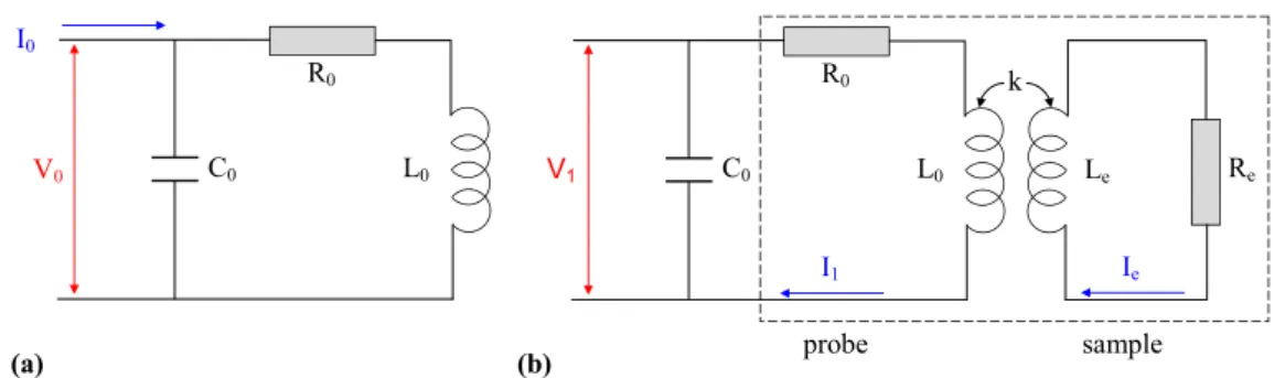
2.14 Schematic diagrams of the equivalent circuit models in air and in the presence of a sample. . . 46

2.15 Comparison of numerical and analytical solutions to the equivalent circuit while neglecting the resistance. . . 51

3.1 Schematic diagram of the scanning procedure used to acquire B-scans. . . 53

3.2 Schematic diagrams of the periodic Lamb wave EMATs. . . 56

3.3 Time domain signal and frequency content of the broadband generation pulse . . . 57

3.4 Time domain signal and frequency content of the narrow-band generation pulse . . 58

3.5 Schematic diagram of the detection EMATs used . . . 58

(9)

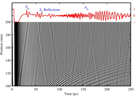
4.2 B-scan results of the broadband measurement. . . 64

4.3 Flow chart of thickness measurement algorithm. . . 65

4.4 Windowed A0waves at two proximate measurement positions. . . 66

4.5 The CSD and unwrapped phase for the broadband measurement . . . 66

4.6 Frequency dependent phase velocity and thickness for the broadband measurement 68 4.7 Measured thickness across the sheet using broadband Lamb waves . . . 68

4.8 Wavelength of the A0wave as a function of frequency in a 100μm thick aluminium sheet . . . 70

4.9 B-scan results of the narrow-band measurement . . . 71

4.10 Thickness prole of a nominally 100 μm thick aluminium sheet using narrow-band signals. . . 73

4.11 Dual channel B-scans of a narrow-band signal . . . 74

4.12 Thickness prole of a nominally 100μm thick aluminium sheet using a dual channel EMAT. . . 75

5.1 Results of the thickness measurements from a 250μm thick aluminium sheet . . . 79

5.2 Results of the thickness measurements from a 500μm thick aluminium sheet . . . 80

5.3 Phase dierence due to the presence of a magnet between the transducers . . . 82

5.4 Change in the thickness prole due to tilt in the detection transducer. . . 83

5.5 Results on thicker aluminium samples using single channel data. . . 84

5.6 B-scans of thickness measurements performed on steel samples . . . 85

5.7 Comparison of the long wavelength approximations to the dispersion curves . . . . 87

5.8 Accuracy of the Lamb approximations for phase velocity of the fundamental modes 87 5.9 Improvement to the long wavelength approximation for the A0wave. . . 88

5.10 Validity of the improved approximation for a single material. . . 89

5.11 Validity of the improved approximation as the material properties vary. . . 91

5.12 Validity of the improved approximation as the transverse and longitudinal velocities vary. . . 92

7.1 Transverse misalignment of the probe on a roller. . . 102

7.2 Equivalent circuit of an eddy coil in proximity to a sample. . . 104

7.3 Comparison of the analytical and numerical models for the resonant frequency and impedance. . . 105

(10)

7.6 Diagrams showing the positional encoding of the probe. . . 109

7.7 Schematic diagram of the upper portion of the high precision lift-o stage. . . 110

7.8 Phase of a coil at resonance . . . 114

7.9 Operation of the frequency counter. . . 115

7.10 Comparison of two resonances with dierent quality factors . . . 116

8.1 Schematic diagram of the racetrack coil used in the single frequency measurements. 118 8.2 Experimental and theoretical impedance response of a coil held above an aluminium sample. . . 119

8.3 Experimental and theoretical resonant frequency changes of a coil held above an aluminium sample. . . 120

8.4 Response of a coil driven using a signal frequency on aluminium. . . 121

8.5 Response of a coil driven using a signal frequency on ferritic steel. . . 121

8.6 Relationship between the measurement number and the lift-o using the precision stage. . . 123

8.7 Phase Dierence results for a measurement at 2 mm lift-o and 0.9 μm resolution. 124 8.8 Reliability of the phase data at 2 mm lift-o and 0.9μm resolution. . . 124

8.9 Reliability of the amplitude data at 2 mm lift-o and 0.9μm resolution. . . 125

8.10 Results for industrial samples with a resolution of 0.9μm. . . 126

8.11 Results for industrial samples with a resolution of 3.0μm. . . 126

8.12 Schematic diagram of the method of examining the sensitivity of the probe to transverse misalignment. . . 127

8.13 Transverse and vertical scans above a curved sample. . . 128

8.14 Calibrated transverse scan above a curved sample. . . 128

9.1 Response of the resonance method on the C40 sample at lift-os up to 10 mm. . . 131

9.2 Reliability of the resonance method on the C40 sample with a resolution of 0.9 μm at a lift-o of 2 mm. . . 132

9.3 Reliability of the resonance method on at industrial samples. . . 133

9.4 Reliability of the resonance method at high lift-os on the C40 sample . . . 134

9.5 Stability of the resonance measurements over a typical measurement time. . . 135

9.6 Transverse performance of the coil driven at resonance. . . 137

9.7 Schematic diagram of dynamic rig. . . 138

9.8 Investigation of the calibration data. . . 139

(11)

9.10 Pictures of the industrial testing apparatus. . . 142

9.11 Prole measurements of the rst roller. . . 143

9.12 Fitted prole measurements of the rst roller. . . 144

9.13 Response of the eddy current probe to liquid. . . 145

9.14 Response of the screened eddy current probe in the presence of liquid. . . 145

9.15 Prole measurement of the second roller . . . 146

9.16 Roundness measurement of the second roller . . . 147

(12)

List of Tables

1.1 Summary of the dierent approaches considered for performing prole measurements. 13

5.1 Changes in separation for the dual coil transducer. . . 81

8.1 Summary of reliability measurements across all samples for the single frequency technique. . . 127

9.1 Summary of reliability measurements across all samples for the resonant frequency technique. . . 134

(13)

Acknowledgements

My greatest thanks must go to my academic supervisor Dr. Rachel Edwards. Without her constant patients, support and proof reading this thesis would be of considerably poorer quality and would have many more typos than it currently does. I must also thank my industrial supervisor Dr. Mark Potter, for his support and friendship throughout my studies, as well as his tolerance of my abuse of the rules of tabletop RPGs. I would also like to thank everyone in the Ultrasonics Group who have been in equal parts helpful, supportive and fun, although I would like to single out both Dr. Phil Petcher and Dr. Charley Fan, for their mentor-ship and unending tolerance of stupid questions. I would also like to thank everyone else in the Department of Physics who have made coee breaks more interesting, and Christmas dinners more entertaining.

I would also like to thank my family for their support (particularly nancial!) during my time at the University of Warwick. A big thanks goes to the members of Warwick Latin and Ballroom Dancesport for welcoming me into the sports club which has dened my last few years at university; my sanity may have long since ed, but I held onto it for slightly longer with your help. I would particularly like to thank my dance partners over the last three years, Daria Gromyko and Ellen Webborn, as they have had to bear the brunt of my personality. There are many other people to whom I owe my gratitude, but naming names would take many more pages, and enough trees have made that sacrice.

(14)

Declaration

I declare that the work presented in this thesis is my own except where stated otherwise, and was carried out entirely at the University of Warwick during the period between October 2010 and September 2014, under the supervision of Dr. Rachel Edwards. The research reported here has not been submitted, either wholly or in part, in this or any other academic institution, for admission to a higher degree. Parts of this work, and other work not reported in this thesis, have appeared in other forms, listed here.

Conference proceedings:

K. L. McAughey, R. S. Edwards, M. D. G. Potter, and S. Dixon,Thickness Measurements of Sub-Millimetre Thickness Foils Using Lamb Wave Dispersion, Submitted Boise (Idaho), USA: 2014.

K. L. McAughey, R. S. Edwards, M. D. G. Potter, and S. Dixon, Ultrasonic Thickness Meas-urements of Sub-millimetre Thickness Sheets, in 18th World Conference on Nondestructive Testing, Durban, South Africa: 2012.

Presentations at national and international conferences:

K. L. McAughey, R. S. Edwards, M. D. G. Potter, and S. Dixon, Thickness Measurements of Sub-Millimetre Thickness Foils Using Lamb Wave Dispersion, presented at the 41st Annual Review of Progress in Quantitative Nondestructive Evaluation (QNDE 2014), Boise (Idaho), USA, July 2014. Poster.

K. L. McAughey, R. S. Edwards, M. D. G. Potter, and S. Dixon, Thickness measurements of sub-millimetre thickness foils using Lamb wave dispersion, presented at the 52nd Annual British Conference on Non-Destructive Testing (NDT 2013), Telford, UK, Sep. 2013. Talk.

(15)

K. L. McAughey, R. S. Edwards, M. D. G. Potter, and S. Dixon, Ultrasonic Thickness Measurements of Sub-millimetre Thick Samples, presented at the 18th World Conference on Nondestructive Testing (WCNDT 2012), Durban, South Africa, April 2012. Talk.

(16)

Abstract

This thesis is concerned with two separate research projects; thickness measurements of sub-millimetre thickness sheets using the dispersion of Lamb waves, and the one dimensional prole measurement of samples with a resolution of 1μm with a dynamic range of 2 mm.

The measurement of the wave velocities of the fundamental Lamb wave modes at long wavelengths is used to calculate the thickness of aluminium sheets without any a priori knowledge of the material properties of the samples being tested. The approximations used to perform these measurements were originally formulated by Lamb and their range of validity is examined, and found to have an upper limit of 14.1 kHz.mm. The reliability of the measurements across a range of sample thicknesses, from 100 to 500 μm. An empirical extension to the approximations

is also presented which greatly extends their range of validity with limited knowledge of the sample properties, to 800 kHz.mm if the longitudinal and transverse sound velocities are known to within 1 % error. As part of this thesis several novel transducer designs for generation of periodic out-of-plane forces suitable for preferentially generating the A0 wave are also presented.

The measurement of the one dimensional prole of a curved sample made of ferritic steel is performed using eddy current measurements. The eddy current probes used in this manner have rst been demonstrated in a laboratory to be capable of measuring a 0.9 μm change in lift-o

at a range of 10 mm with a reliability of 90 %. These probes have also been demonstrated to be insensitive to transverse misalignment of ±1 mm to the curved sample. Further to these measurements the system has also been used in eld trials at a the site of an industrial partner using custom hardware and software developed during the course of this research. These measurements allow the recreation of the prole of samples within 10μm of the current standard and have been

(17)

Abbreviations

2D-FFT Two-Dimensional Fast Fourier Transform AC Alternating Current

AFM Atomic Force Microscopy ADC Analogue to Digital Converter CSD Cross Spectral Density CT Computed Tomography DC Direct Current

DD Dierence Detection DFT Discrete Fourier Transform

EMAT ElectroMagnetic Acoustic Transducer FFT Fast Fourier Transform

FT Fourier Transform

LCR Circuit with capacitor, inductor and resistor NDE Non-Destructive Evaluation

NDT Non-Destructive Testing PDS Phase Dierence Spectrum PPM Periodic Permanent Magnet SH Shear Horizontal

(18)

Chapter 1

Introduction

This thesis consists of two separate research projects using electromagnetic sensors for non-destructive evaluation (NDE). The rst is the use of electromagnetic acoustic transducers (EMATs) to generate and detect ultrasonic guided waves in thin samples, and from this determine the thicknesses of the samples. The specics of this work is discussed in chapters 3-6. The second project was performed as a piece of commercial research, and so many of the details presented within this thesis remain condential. This research focused on the use of eddy current coils to perform prole measurements to an accuracy of 1μm, and in the unredacted version of this thesis

details are discussed in chapters 7-10. An overview of the theory for both projects is given in chapter 2, while this chapter introduces the measurement techniques and describes the current state of the art.

1.1 General introduction to NDE

Non-destructive evaluation (often used interchangeably with the term non-destructive testing, or NDT) is a discipline which aims to address the necessity of inspecting components without damaging them [13]. These inspections fall into a range of categories, such as aw detection and residual stress measurements [2,4], and there is some overlap with the related eld of metrology for thickness or prole measurements [57]. There are a large number of methods employed in NDE inspections, including thermal, radiographical, optical, electromagnetic and ultrasonic techniques, where each technique has advantages and disadvantages, leading to some techniques being more suitable for specic applications.

(19)

of the art for thickness measurements, including using guided ultrasonic waves is discussed in section 1.2, while the theory is given in sections 2.1 and 2.2. An introduction to prole measurements is given in section 1.3, while the theory of using eddy currents to perform lift-o measurements is given in section 2.5.

1.2 Thickness Measurements

The rst of the two research projects discussed in this thesis covers thickness measurements of sub-millimetre thickness sheets. Thickness measurements form a key part of NDE, both during the manufacture of components as diverse as gas turbine blades and drinks cans as a form of quality assurance [8], and during the life of the component as a method of detecting damage due to corrosion [9]. Moreover, the range of thicknesses investigated can vary from a few hundred microns to several meters.

1.2.1 Research Problem and motivation for the research

Although thickness measurements cover a very broad eld and form a well established branch of NDE, this research aims to expand the eld by developing a technique capable of perform-ing thickness measurements on sub-millimetre thickness samples without prior knowledge of the material properties of the sample. The technique proposed would allow thin foils, typically the product of cold-rolling [10], to have their thickness measured ultrasonically without the texture of the roll aecting the measurement [11]. This would allow the radiographic methods which are typically used to be replaced with an intrinsically safe, and calibrationless, ultrasonic method. This replacement would remove the need for users to comply with the large amount health and safety legislation relating to radiographic inspection [12]. The proposed technique could also match on the accuracy of a commercial radiographic system, typically 1μm [13]. This technique would also

have applications to measurements of the wall thickness of drinks cans, as these often have large amounts of texture due to the way they are manufactured [10]. This allows the integrity of the can to be inspected, and reduces the likelihood of the can failing and spilling its contents. Current methods of thickness gauging are discussed here.

1.2.2 Electromagnetic NDE

(20)

quantication of the electrical properties of materials [1518]. As the depth of penetration of an electromagnetic eld into a conductive sample is limited by the skin depth [19], typically in the order of a few hundred microns, these methods are primarily used for surface inspections.

Eddy current testing has previously been used for thickness measurements of both copper and aluminium samples, both in free space and when in the presence of a substrate [18]. In these measurements the impedance of a cylindrical coil held above an electrically conductive sample was measured using an impedance analyser, and an inverse method was used to identify the values of thickness and conductivity at which the impedance of an analytical model most closely matched the experimentally measured impedance. Provided that the sample thickness was between a fth and half of the radius of the coil both the thickness and the conductivity could be calculated, although for thinner samples at least one of the parameters is required to be known in order to accurately evaluate the analytical solution. However, the thickness estimates from this measurement technique, typically being within 10 % of the actual thickness, are not consistently accurate across the range of samples measured, with the performance of the measurement on an aluminium sample in air being particularly unreliable, consistently producing errors greater than 17 % [18].

A more recent experiment, which aimed to simultaneously measure both the lift-o and thick-ness of both aluminium and copper sheets, produced signicantly more accurate results [20]. These experiments were conducted with a similar cylindrical coil to those mentioned previously, and the same approach of utilising an inverse method was made. In this research, however, the inverse model was simplied using knowledge of the material properties, although the lift-o between the coil and the sample was also used as a variable. The impedance of the coil was measured using an impedance analyser and the analytical solution was evaluated for various values of sample thickness and lift-o in order to most closely match the experimental results. Using this method the accuracy of the thickness measurements on copper samples was approximately 5 % over a range of thicknesses from 22 to 110μm. The accuracy on the aluminium samples was less consistent, varying between 1

and 17 % over samples ranging from 18 to 108μm thick. While this shows a large improvement over

the previous thickness measurements using eddy currents, the measurement technique still requires accurate knowledge of the electrical properties of the sample. Additionally, the accuracy achieved here is not sucient for the intended industrial application, where a tolerance of approximately 1 % is believed to be necessary. Indeed, for non-ferritic materials thicker than 100μm the accuracy

(21)

1.2.3 Radiography

Radiography is typically used to investigate the bulk of a sample, and the eld consists of several similar techniques, using x-rays, gamma rays or, occasionally, neutrons [22, 23]. Radiographical techniques are often used for detecting defects within the bulk of a material, particularly when inspection using other methods is dicult or provides poor results, such as the inspection of concrete [24].

Thickness measurements can be made using a type of radiography which was rst used in medicine, known as computed tomography (CT) [25], and this has also been used industrially [26]. In these measurements a large number of images are captured at dierent angles through the same sample, and these individual images are then combined to form a three dimensional model of the component being inspected. Due to the large number of individual images needed CT measurements can take a large amount of time to perform, and the use of even basic radiography is heavily legislated due to the health risks involved.

A more basic method of measuring the thickness of foils during manufacture using radiography exists, and is widely used [10]. In this method a beta radiation source is placed on the opposite side of the foil from a detector, and the intensity of radiation detected is related to the thickness of the foil by

I=I0e−µx, (1.1)

where I0 is the intensity when no foil is present, µ is the coecient of attenuation, andxis the thickness of the foil [27]. The intensity measured using this technique is often used as a feedback control for the rolling process, so that the foil produced is of consistent thickness. However, the coecient of attenuation for the material must be known in order to perform this measurement, which is a limitation compared to the technique proposed which requires no a priori knowledge of the material properties of the sample.

1.2.4 Thermography

Thermography uses the ow of thermal energy in a sample to extract information about the sample, and is often used to detect defects such as impact damage or delaminations in composite materials [3]. Thermography can also be used to perform thickness measurements. These are done by heating a sample and then recording images of the sample as it cools using a thermal imaging camera, where the rate of dissipation of the heat in the sample can be used to calculate relative thickness proles. For coatings of thicknesses between 50 and 400 μm on a substrate the time

(22)

the thickness, and can be used to successfully dierentiate between adjacent areas with dierent coating thicknesses [28]. Due to the nature of the exponential decay of the thermal energy in the sample the dierence between the thicker 400μm coating and the 300μm coating is much more

apparent than the dierence between the 300 μm coating and the 200 μm coating. However, the

coatings in this measurement were paints with a low value of thermal conductivity, and as such the measurement is not likely to be directly transferable to a highly thermally conductive material such as aluminium.

Thermography has also been used to characterise material loss due to corrosion in thicker metal samples [29]. In this study a plate with a number of test defects was heated using a quartz lamp heater, activated for a ve second pulse. The cooling of the sample was then monitored using a thermal imaging camera, and the hotspots in the image were used to identify the defects, while the times at which these hotspots appeared can be used to measure the depth of the defect. Using this technique regions of 10 % wall loss can be detected in a sample with a nominal thickness of 3 mm, and the areas of wall loss can be eectively sized. However, for thicker samples the lateral heat conduction in the plane of the sample makes the measurements less accurate, and in samples of up to 5 mm nominal thickness the lower limit of detectable wall loss is increased to 25 %. Thickness measurements with an accuracy in the order of 1 % of the sample thickness may be beyond the ability of most thermographic methods, in addition to which the required knowledge of the thermal conductivity of the sample limits the technique.

1.2.5 Ultrasonics

Ultrasonics is a broad eld relying on the behaviour of the propagation of sound in a material to infer information about that material. While this has applications to thickness measurements [2,6], ultrasonics can also be used for defect detection and stress measurements [3032]. This section introduces a number of the applications for which ultrasound can be used, and also discusses some of the methods of generating and detecting ultrasound in a sample. The dierence between bulk waves and guided waves for ultrasonics is discussed in greater detail in chapter 2, although the key dierence is that guided waves are ultrasonic waves which are geometrically constrained by the medium in which they are propagating. The applications of these waves to thickness measurements will also be discussed in chapter 2.

1.2.5.1 Bulk wave methods

(23)

are the most common type of ultrasonic measurements, and in addition to their use in thickness measurements they can also be applied to aw detection and array based ultrasonics [2, 33]. For simple aw detection, time of ight measurements can give the distance a particular aw is located from the transducer, while the amplitude of the reected signal can determine the lateral extent of the defect using the 6 dB drop method [34]. By using arrays of transducers it is possible to locate the defects more precisely by comparing the time of ight of the reected signal for dierent elements in the array. In addition to simple aw detection other more advanced techniques exist to determine the size of defects within the sample, such as time of ight diraction (ToFD) [30], where the diraction from the tips of cracks is used to determine the size and position of defects with an extremely high level of accuracy.

Another application of bulk wave ultrasonics is for the characterisation of stress within a sample, which is typically done via non-linear analysis of super-harmonics of a generated wave [4, 35]. By investigating the intensity of the second order harmonics it is possible to detect and quantify the material fatigue in metal samples, before cracks or other defects begin to form in the sample.

1.2.5.2 Guided wave methods

Guided waves can be used for many of the same applications as bulk waves, such as aw detection or measurements of non-linearity [32,36], although there are advantages and disadvantages to their use. Due to the conned nature of guided waves they can propagate over much greater distances than bulk waves, in some cases over a kilometre [37], and this gives them a distinct advantage in being able to inspect large areas quickly and remotely. However, this capability comes at a cost, in that guided waves are often less eective at locating and sizing defects when compared to bulk wave methods. A further disadvantage of guided waves is that the signals received are often complicated by the presence of multiple wavemodes, due to the existence of multiple solutions to the guided wave equations (section 2.2) [38]. There are two common approaches to overcoming this problem, either through physically optimising the transducers to preferentially generate and detect a single wavemode [39], or through advanced signal processing which is capable of decomposing the various wavemodes [40].

(24)

near-eld of the guided wave allow greater opportunities for characterisation of defects, in both their size and orientation [43, 46]. By analysing the frequency of the wave which is transmitted past the defect it is possible to estimate its vertical extent, while the enhancement of either of a laser generated guided wave as either the laser source or laser interferometer passes over the defect can provide information about its angle to the surface [48]. The sensitivity of guided wave inspections in defect characterisation can also be improved by applying tomographical reconstruction [49,50], which operates in the same way as CT scanning, where the combination of multiple views through a sample allow much more precise imaging of defects than available through conventional guided wave inspections.

As with bulk waves, surface guided waves have also been used for non-linearity measurements in order to determine the eects of stress on samples [32, 51], these studies present two dierent approaches to non-linear measurements. In [32] a low frequency pump wave is used to load the sample while a high frequency wave is used to interrogate it for non-linear response; the low frequency wave introduces a change in the velocity of the material by introducing a non-linearity into the sample. The change in the velocity of the high frequency probe wave is then used to make an assessment of the non-linearity in the sample. In [51] a single wave is used, where the ratio of the amplitude of the rst and second order harmonics for the narrow-band Rayleigh wave is used to asses the non-linearity of the sample. In both cases the acoustic non-linearity of the sample can be related to either the stress or strain in the sample, allowing a measurement of the fatigue damage before any macroscopic cracks are present.

(25)

measurements [59].

One of these studies explores an approximation that gives a direct relationship between the wave velocities of Lamb waves within a sample and the thickness of the sample [55]. By using approximate values for the velocities of the fundamental Lamb waves at low values of frequency thickness an equation is given which relates these velocities to the frequency of the Lamb waves and the thickness of the sample. This is described mathematically and discussed in detail in section 2.2.3, where a critical review of this method is also given, and is the basis for the research into thickness measurements using Lamb waves presented in this thesis. A similar technique, using the dispersive properties of SH guided waves [62] to perform calibrationless thickness measurements, has also been reported. Thickness measurements of samples below 1 mm in thickness have not been reported, although the error is reported to increase for thinner samples or measurements at longer wavelengths [62].

1.2.5.3 Transduction of guided waves

A number of methods exist for generating and detecting ultrasound, and these are discussed in this section, with a particular focus on their application to generate Lamb waves. The rst such method is that of piezoelectric transducers, which rely on the piezoelectric eect discovered in quartz by Jacques and Pierre Curie [63]. Piezoelectrics are a class of crystals which undergo strain when a voltage is applied to them [64]. This is due to the noncentrosymmetric nature of these crystals, where the arrangement of the atoms in the crystal lattice creates an electric dipole which shifts when exposed to an electric eld. Man-made piezoelectric materials, such as lead zirconium titanate (PZT), often belong to a class of crystals known as ferroelectrics. The piezoelectricity in these crystals arises from a dipole present in the crystal, where one of the atoms of which the crystal is composed is not in the centre of the crystal [64]. However, like the ferromagnetic materials after which they have been named, ferroelectric materials only retain their properties up to a maximum temperature, the Curie temperature (Tc), limiting the temperature range in which the transducer

can be used eectively [65].

(26)

mechanically clamped to the surface of the sample, in this case with steel or brass shim between the sample and transducer, in order to couple ultrasound eciently into the sample. These contact methods typically oer more ecient transduction than non-contact methods [67], resulting in higher signal to noise ratios. However, when generating and detecting ultrasound in very thin samples non-contact methods are often preferred as they avoid altering the sample which is being measured due to surface loading [68]. Non-contact measurements also allow the measurements to be performed in hostile environments, where piezoelectric transducers are unsuitable [8].

One non-contact method is that of laser based ultrasonics [69]. Although a piezoelectric transducer is reversible, that is the detection method is the inverse of the generation method, this is not true for lasers, which require two separate systems for generation and detection. For generation a high power laser is directed at the sample in order to generate ultrasound. In general this can be done in one of two ways; with a suciently powerful laser the point on the surface of the sample on which the laser is focused is ablated and becomes a plasma, which rapidly expands and impacts the sample, creating an ultrasonic pulse. By reducing the power of the laser, the sample at the focal point can simply be heated, and the corresponding thermal expansion provides the ultrasonic pulse [69]. These methods of generation are known as the ablative and thermoelastic regimes respectively. Detection of ultrasound using lasers in academia is typically achieved using an interferometer, as discussed in [59], although vibrometers can also be used [70], and are more common in industrial applications. These systems typically detect the vertical displacement of the surface of a sample by measuring the eect the moving sample has on the phase of a beam of light generated by a laser, although methods also exist to detect vibration in the plane of the sample as well [71]. Laser ultrasound systems can operate at large distances from the samples which they inspect, making them ideal for remote applications where the conditions which the sample is under are inimical to other transducers [72], and have been used to generate and detect Lamb waves [5557,59,60,73]. Laser based ultrasonic systems have also been used to perform inspections in inimical environments, such as the thickness measurements of steel at temperatures of up to 1250 ºC [74].

(27)

usually the Lorentz force still remains the main method of coupling ultrasound into the sample [78]. Although EMATs cannot operate at the same distance from the sample as lasers, they can still operate remotely, although the eciency of the transducer decreases rapidly with increasing lift-o. Another consequence of increasing the lift-o of a transducer is that this can eect the phase of the signal recorded by the transducer [79], which can lead to errors in experimental measurements if the separation between the sample and the transducer is not kept constant. EMATs are considerably less expensive than lasers, and the conguration of the coil, static magnetic eld, and current pulse can be designed to produce narrow-band signals.

1.3 Prole measurements

The second research project in this thesis concerns the measurement of the prole of a sample along its length, aiming to detect changes in the sample height of 1μm over a dynamic range of at

least 2 mm. Accurate surface prole measurements are an important part of the quality assurance of many components, and this is a eld which has relevance in both NDE and metrology [80, 81]. These prole measurements are used in a number of industries for detection of warping or bending of manufactured components [7], as well as to measure structures in situ, such as continuity of road surfaces [82].

1.3.1 Research problem

The measurement of proles is a well discussed eld and several competing technologies exist. Due to the commercially sensitive nature of this work the exact nature of the research problem is discussed in detail in chapter 7. However, the research problem distils to a one dimensional measurement of the surface prole of a metal sample, where the electrical properties of the sample are signicant as they allow electromagnetic methods to be considered. The accuracy of the system must be sucient to resolve changes in lift-o of 1 μm, while operating over a range of at least

2 mm. While this can be achieved using existing contact measurements, a non-contact method is preferred to preserve the surface nish of the sample under test.

1.3.2 Contact measurements

(28)

commonly used in industry to measure surface proles due to the simple nature of the measurement, and are the subject of industrial standards [84]. A limitation of these contact measurements can arise from the jitter in the stylus as it moves across the surface of the sample, although this can be alleviated by applying lters to the acquired data [83]. Due to the contact between the tip and the sample, the tip can also cause damage the surface nish of the sample, particularly where the nish is highly polished.

A similar, but signicantly more precise method of determining the surface prole is by using atomic force microscopy (AFM), which allows resolution of the surface prole to an atomic scale [85]. It should be noted that although the AFM can be used as a contact measurement, it can also be used in a non-contact mode as well, where the van der Waals force from the surface of the sample acts on the tip, causing it to deect without contact [86]. However, the limited scanning area and delicacy of the system preclude the use of AFM in almost all industrial environments. [7]

1.3.3 Optical measurements

Optical measurements are also used extensively to perform prole measurements, as well as to determine the surface roughness of samples [87]. This can be done in a number of ways, such as interferometry or by pattern projection [7,88]. These methods often have a very high throughput, allowing large areas to be inspected and proled in very little time. In one study, a pattern projection method, where a known pattern of light is applied to a sample of unknown topography using a projector in order to measure the deviation of the pattern and calculate the topography, was used to calculate the topography of silicon wafers to an accuracy of 50μm. This accuracy was

achieved using a system which could analyse over 2000 silicon wafers per hour, making it extremely useful for on-line monitoring [7].

The ability to scan large areas in one measurement is a signicant advantage for pattern projection type measurements over those relying on stylus based contact measurements or those using interferometry, as these latter methods must be raster scanned over the desired area to be inspected. The disadvantage of these optical systems is that the surface condition of the sample is key to the performance of the system, where interferometry often requires a reective sample in order to function with high accuracy.

1.3.4 Electromagnetic methods

(29)

between the probe and the sample. This dependence allows the lift-o of the probe from the sample to be determined, and if the probe is maintained at a xed height above the sample, allows the prole to be calculated. There are two main methods of prole measurements using electromagnetic sensors; capacitive measurements and inductive measurements, and each will be discussed in the following sections.

1.3.4.1 Capacitive methods

Capacitive measurements are based on the change in the capacitance of a measurement probe [1]. In the simplest possible case for a probe used to measure lift-o, the conductive sample acts as one electrode while a metal plate on the probe acts as the other, eectively creating a capacitor between the probe and the sample [14]. The capacitance of this probe will vary with the lift-o of the probe,

C= Aε

d , (1.2)

where A is the area of the metal plates,ε is the permittivity of air, andd is the lift-o between

the probe and the sample. However, in order to achieve a high spatial resolution the capacitive plate of the probe must be as small as possible, which increases the dominance of edge eects on the measurement [89]. Other capacitive probes can achieve greater range and sensitivity by utilising these fringe eects by sensing the change in capacitance between two concentric rings [90]. This proximity measurement, while extremely accurate over small values of lift-o, becomes less accurate as the lift-o increases beyond 200 μm.

1.3.4.2 Inductive methods

Inductive methods involve measuring a change in the inductance of a coil which is in proximity to an electrically conductive sample when an alternating current is applied to the coil. This change is caused by the time varying magnetic eld in the coil inducing an electrical current in the surface of the sample, known as an eddy current [27,91]. The inductive coupling between the coil and the sample will cause a change in the impedance of the coil as the lift-o between the sample and the coil is altered, where this impedance change can be quantied by taking the ratio of the voltage across the coil to the current owing through the coil [92]. The relationship between lift-o and impedance change is discussed in greater detail in section 2.5.

(30)

application of prole measurements this eect is key to determining the lift-o of samples from the eddy current probe. Measurements of the lift-o for both copper and aluminium sheets have previously been conducted simultaneously with measurements of the sheet thickness, typically to accuracies of greater than 96 % at lift-o ranges of up to 2 mm by investigating the change in the impedance across the entire frequency range of a coil [20]. In a more recent study by the same authors both the accuracy and range of the measurement have been improved, with accuracies of greater than 98 % achieved at lift-o ranges of up to 4 mm on aluminium [96].

Due to this large operational range, combined with the promising accuracy of the measurement and the relative insensitivity of the measurement to the surface condition of the sample, an eddy current based system was chosen to be developed into a measurement tool capable of meeting the requirements of the industrial research. The resolution in the lift-o measurements which these probes are capable of detecting must be improved to a level of 99.95 % in order to detect a 1 μm

change at a lift-o of 2 mm. Additionally, the measurement system developed must be robust enough to work eectively in an industrial environment.

A brief summary of the methods considered is shown in table 1.1, where the eddy current approach overcomes the limitations of the other techniques.

Technique Benets Limitations

Contact Direct measurement of sample prole Can cause damage to sample Optical Extremely high resolution measurements Requires clean surface nish Capacitive Very high sensitivity to lift-o Very short operating range

Inductive High operating range Susceptible to material variations

(31)

Chapter 2

Theory of high precision

measurements

This chapter covers the theories behind the research described in this thesis, including the ultrasonic generation and propagation of Lamb waves, the equivalent circuit model of eddy current interaction, and an overview of some of the signal processing techniques used during the data processing. Due to the transition between physical and electrical phenomena there are some small changes in the notation between sections 2.1 and 2.2 covering ultrasonics, and sections 2.3 and 2.5 covering EMATs and eddy currents. Where such changes in notation occur it will be explicitly noted.

2.1 Ultrasonic Waves

(32)

follow the same constituent equations as bulk waves [38], although the nature of the solutions to the wave equations will change depending on the boundary conditions which dene the guided wave (discussed in section 2.2).

This section focuses on the mathematical description of an ultrasonic wave in an elastic solid, initially considering bulk waves. The methods of using bulk waves to perform thickness meas-urements are also discussed. In addition, the eect of boundary conditions on the propagation of ultrasonic waves in thin sheets is considered as part of the mathematical description of Lamb waves in section 2.2, while their applications to thickness measurements are examined in section 2.2.3.

2.1.1 Propagation of ultrasound in isotropic solids

When considering the propagation of ultrasound in a solid medium, the simplest case is that of an isotropic and homogeneous solid with no boundary conditions. In such a material the speed of propagation is independent of the direction due to the isotropy of the medium, and the homogeneity ensures that the propagation behaviour is the same regardless of location [98]. Another consideration in the mathematical description of the propagating ultrasound is the type of deformation caused by the travelling wave. Ultrasound waves used in NDE are, by denition, of relatively small amplitudes, such that the particle motion of the solid does not exceed the elastic limit. This is important as any violation of Hooke's law would destructively deform the sample under examination [2]. In this section the subscript tensor notation with the summation convention is used, commonly known as Einstein notation [99], and partial derivatives of tensors with respect to spatial dimensions are expressed in full, e.g. as ∂ui

∂xj rather thanui,j. Vectors are expressed using

arrow notation, ~u, and dierentials with respect to time are also expressed in full in both tensor

and vector notation, ∂ui ∂t or

∂2~u dt2.

2.1.1.1 Relationship between stress and strain

The propagation of ultrasonic waves in an isotropic solid is governed by the relationship between the stress and strain in the solid. Due to the small amplitudes of ultrasonic waves used for NDE, the relationship between the strain and the particle displacement can be written in the following form [98],

εij= 1 2

_∂u

i

∂xj +∂uj

∂xi

, (2.1)

where εij is the tensor strain, uis the particle displacement and xis the direction of the strain.

(33)

formulation of the strain tensor is known as the Cauchy strain tensor, and can be expanded to the following form for a three dimensional system,

εij =       ∂u1 ∂x1 1 2 ∂u1 ∂x2 +

∂u2 ∂x1 1 2 ∂u1 ∂x3 +

∂u3 ∂x1 1 2 ∂u2 ∂x1 +

∂u1 ∂x2 ∂u2 ∂x2 1 2 ∂u2 ∂x3 +

∂u3 ∂x2 1 2 ∂u3 ∂x1 +

∂u1 ∂x3 1 2 ∂u3 ∂x2 +

∂u2 ∂x3 ∂u3 ∂x3       . (2.2)

The Cauchy strain tensor is symmetric and hence εij = εji. This stain tensor is related to the

stress tensorσij for a general material using,

σij =cijklεkl, (2.3)

where the tensorcijkl is a fourth order tensor known as the stiness tensor. When considering an

isotropic material this equation can be greatly simplied to [38],

σij =λεkkδij+ 2µεij, (2.4)

where λand µare the two Lamé coecients of the material [98]. The term εkk is known as the

dilatation [38,98], where the repeated indexkdenotes that only the trace of the tensorεij is being

considered. The dilatation is also represented by ein some literature [53, 98], and is the relative

volume change of the material under strain, and is variously dened as,

e= ∆V

V0

=εijδij. (2.5)

where∆V is the change in volume due to the strain in the material,V0 is the original volume and

δij is the Kronecker delta. Equation 2.4 can then be rewritten substituting the denition of the

strain from equation 2.1,

σij =λ

∂uk

∂xk

δij+µ

_∂u

i

∂xj +∂uj

∂xi

. (2.6)

2.1.1.2 Dynamic motion in elastic media

(34)

of ultrasonic waves in a medium, the tensor form of Newton's third law of motion is considered [53],

∂σij

∂xj

+ρfi=ρ

∂2_u

i

∂t2 , (2.7)

where ρ is the density and fi is the body force per unit mass. The body forces encompass

gravity and other forces that act throughout the material, and for a material in a state of general equilibrium this can be ignored. By omitting the body forces term this equation can be rewritten, substituting the relationship between the stress tensor and the particle motion given in equation 2.6, to arrive at the Navier-Cauchy governing equation, which can be expressed in tensor form as [38, 53],

µ∂

2_u

i

∂x2_j + (λ+µ) ∂2_u

j

∂xj∂xi

= ρ∂

2_u

i

∂t2 . (2.8)

As this equation consists only of rst order tensors it can also be denoted using vector notation, where the del operator,∇, is used in place of spatial dierentials,

µ∇2_~_u_{+ (}_λ₊_µ₎_{∇∇ ·}_~_u₌_ρ∂ 2_~_u

dt2, (2.9)

allowing a simpler expression of the equation. In order to further simplify the equation, the vector

~

ucan be subjected to Helmholtz decomposition in order to be stated in terms of a vector potential

and a scalar potential [97],

~

u=∇φ+∇ ×ψ.~ (2.10)

This decomposition allows the Navier equation to be rewritten in terms of two uncoupled potentials, representing the scalar, or dilatational, and the vector, or distortional, components of the vector~u

[53],

∇

(λ+ 2µ)∇2_φ₋_ρ∂ 2_φ

∂t2

+∇ ×

"

µ∇2_ψ_~₋_ρ∂ 2_ψ_~

∂t2

#

= 0. (2.11)

The only valid, non-trivial, solutions of this equation require that both the scalar and vector potential components of 2.11 are equal to zero, which allows the formulation of two separate wave equations,

(λ+ 2µ)∇2_φ ₌ _ρ∂2φ

∂t2 (2.12)

µ∇2_ψ_~ ₌ _ρ∂2ψ~

(35)

The wave described by equation 2.12 is the dilatational wave, which alters the volume of the mater-ial as it propagates, travelling as a wave with alternating regions of compression and rarefaction in the same direction as the propagation [53]. This wave is more commonly known as the longitudinal wave, and its propagation velocity can be determined from equation 2.12 to be,

CL = s

(λ+ 2µ)

ρ , (2.14)

where C is the velocity of the wave and the subscriptL denotes the longitudinal mode [38]. The

velocity of the distortional wave, which is more commonly known as the transverse wave, can also be calculated from its governing equation, equation 2.13, to be

CT =

r_µ

ρ, (2.15)

where the subscriptT denotes the transverse velocity in a material.

This simple derivation of the propagation velocities of the longitudinal and transverse bulk waves is only valid when considering isotropic media, as in an anisotropic medium the stiness tensor (equation 2.3) is considerably more complex. This additional complexity would add a directional component to the derived wave velocities, where the velocity along each of the principal directions of the material would be dierent [97]. The materials considered in this research can be treated as isotropic, and as such this extra level of complexity can be ignored.

2.1.1.3 Phase and group velocity

A propagating wave has two dierent velocities which represent dierent information about the wave, a group velocity and a phase velocity, although these velocities can be equal [100]. The group velocity is the easiest to conceptualise, and is taken to be the propagation velocity of the wave, or the velocity at which energy is transferred by the wave. This is shown in gure 2.1, where the propagation of energy within the wave is given by the propagation of the envelope of the wave and is usually measured by the arrival time of the wave. The phase velocity is the rate at which the phase of the wave propagates, i.e. the rate at which a single peak or trough in the wave packet travels as the wave propagates, and this may be dierent from the group velocity [101]. This concept is visualised in gure 2.1, where the phase velocity is shown by the rate of propagation of a single peak within the envelope of the wave.

(36)

0 500 1000 1500 2000 −2

−1 0 1 2

Time (Arb. Units)

Amplitude (Arb. Units) Group Velocity

Phase Velocity

Figure 2.1: Representation of the dierence between the group velocity, which measures the rate at which the envelope or energy of a wave, shown in red, propagates, and the phase velocity, which measures the rate at which a single peak within the wave packet propagates.

The group and phase velocities can be written as Cg and Cp where the subscript indicates the

group or phase, and the mathematical description of the group and phase velocities is

Cg =

∂ω

∂k, (2.16)

Cp =

ω

k, (2.17)

whereω is the angular frequency of the wave andkis its wavenumber [100]. From equations 2.14

and 2.15 it can be seen that the group velocities of the bulk waves do not depend on the frequency of the wave, but only on the material in which they propagate. Thus the group and phase velocities of the waves are equivalent, and these waves are non-dispersive. The distinction between the phase velocity and the group velocity is extremely important in the discussions of dispersive waves, such as Lamb waves.

2.1.2 Using bulk waves for thickness measurements

(37)

(a) (b)

0 20 40 60

−100 −50 0 50 100

Time (µs)

Amplitude (mV)

1st

2nd

3rd

Pulse Duration Dead Time

Figure 2.2: (a) A schematic diagram of a pulse echo thickness measurement, and (b) an example A-scan measured using this arrangement.

2.1.2.1 Time of ight measurements

Thickness measurements using time of ight are the simplest form of ultrasonic thickness meas-urement, and rely upon calculating the path length of an ultrasonic wave propagating in a sample using the time of ight of the wave and prior knowledge of the wave velocity [2]. A pulse-echo arrangement for measuring thickness is shown in gure 2.2 (a), where the transducer acts as both generator and detector, transmitting ultrasound into the sample and recording the returning echoes from the back wall of the sample. An example of the data recorded using such an arrangement is shown in gure 2.2 (b), using an undamped piezoelectric transducer excited with a broadband source to measure the thickness of an aluminium sample. For the experimental set-up shown in the gure, the thickness of the sample, d, can be determined from the arrival time of the ultrasound

wave at the transducer,

d=Ct

2 , (2.18)

where t is the measured transit time of the ultrasonic wave. Ultrasonic thickness measurements

(38)

thickness measurements on thinner samples. These delay lines often take the form of a physical rod, or an immersion tank, in industrial settings [6], although the characteristics of the delay line must be well understood.

There is an additional limit on the lowest thickness of a sample which can be measured using time of ight measurements, which is the ability to resolve successive back wall echoes. This is a distinct problem from the arrival of the rst back wall echo in the dead time, and cannot be overcome using a delay line. In gure 2.2 (b) the successive echoes are clear and distinct, but in a thinner sample these echoes may start to merge, which will make it impossible to measure the thickness of the sample in the time domain. From this the limit on the thickness and pulse duration is set, such that the duration of the ultrasonic signal, labelled in gure 2.2 (b), must be less than or equal to the propagation time of one round-trip of the wave through the sample. If the ultrasonic wave consists of one cycle at the generated frequency, which is not wholly realistic, as discussed later, then the minimum measurable sample thickness is given by,

dmin=

C

2f, (2.19)

where centralf is the frequency of the generated ultrasound. Hence increasing the frequency will

reduce the minimum thickness of the sample which can be measured.

A reduction in the minimum measurable thickness can also be achieved by using transverse waves rather than longitudinal waves, which travel more slowly than longitudinal waves. This increases the time taken for the ultrasound to propagate through the sample, allowing thinner materials to be measured at the same frequency. However, transverse waves can be dicult to generate eectively using piezoelectric transducers due to the diculty of coupling shear forces through a uid medium [2]. Another method for reducing the minimum thickness which can be measured is by shortening the length of the ultrasonic pulse, for example by using broadband excitation [103], which is typically used in industry. These excitations are similar to a Dirac impulse, with broad frequency content occurring in a small window in the time domain. This eectively allows equation 2.19 to be superseded, as the minimum measurable thickness will be related to both the pulse width,tp, and the speed of sound in the material,

dmin=

Ctp

2 . (2.20)

(39)

First Harmonic

Second Harmonic d

Figure 2.3: Through-thickness resonances for the rst and second harmonics.

of which are experimentally achievable [6]. Any delay in the response of the system will aect the measurement of the thickness if just the rst backwall echo is used (gure 2.2 (b)), as any delay will articially increase the perceived thickness of the sample. A constant delay in the measurement system can be overcome by measuring the time between successive backwall echoes, as the delay will be applied to each echo and will be ignored when looking at the dierential time between echoes. However, for increasingly short pulses in increasingly thin materials the data acquisition hardware may have insucient bandwidth to distinguish between echoes [104]. Thus the actual minimum measurable thickness will be limited by the available hardware, as well as the physical constraints described in equations 2.19 and 2.20.

2.1.2.2 Measurements in the frequency domain

In order to overcome some of the limitations of experimental hardware, thickness measurements can instead be performed in the frequency domain, by measuring the resonant frequency of a through-thickness mode of the sheet [68, 105], i.e. the frequency of the standing waves that occur through the thickness of the sheet. The rst and second harmonics of the through-thickness mode for a sample of thickness dare shown in gure 2.3. This method has been implemented in two

dierent ways, using a frequency scanning approach [68], and using a broadband measurement system [105]. The relationship between the resonant frequency of a through thickness mode and the thickness of the sample is described by

d= C 2f0

, (2.21)

(40)

In the frequency scanning approach a long pulse of energy at a given frequency is introduced to the sample using an electromagnetic acoustic transducer, and the vibration of the plate at that frequency is recorded using the same transducer. In these measurements an EMAT is used to avoid altering the resonance of the sample by loading the surface, as would occur when using a piezoelectric transducer [68,105]. By recording the response of the plate at a number of frequencies a plot of the resonance modes of the plate can determined. Equation 2.21 can then be used to determine the thickness of the sample [68], after identifying the frequency of the rst resonance mode. In the broadband approach a high bandwidth pulse is introduced to the sample using an EMAT, which then records the response of the sample. The A-scans are windowed to exclude the dead time caused by the generation pulse, and then analysed using a Fourier transform. The peaks in the Fourier transforms correspond to the through-thickness resonance modes of the plates, and the frequency of the rst resonance mode can then be used with equation 2.21 in order to calculate the thickness of the sample [105].

This is a general technique, and can be applied to the measurement of coatings and substrates as well as single materials [105]. However, this method has the same fundamental limitation as the time domain measurements in section 2.1.2.1, in that the accuracy of the measurement is dependent on the accuracy to which the speed of sound in the material is known, where this can be aected by the temperature or the composition of the sample [38,106].

2.2 Lamb Waves

Lamb waves are a type of ultrasonic wave that propagate in thin materials, where the wavelength is comparable to the thickness of the propagating medium, and result from the superposition of multiple reected bulk waves which are conned in a thin waveguide. These waves were rst described by Lamb in 1917 [107], and have been the subject of a great deal of research for application in both thickness measurements [5461], and aw detection [36, 47]. Although the multi-modal nature of Lamb waves is extremely complex, the characteristic equations which describe them can be derived from applying the boundary conditions for a thin sample with traction-free surfaces to equations 2.12 and 2.13.

2.2.1 Deriving the characteristic equation

(41)

x

₁

x

₃

h

-

h

d

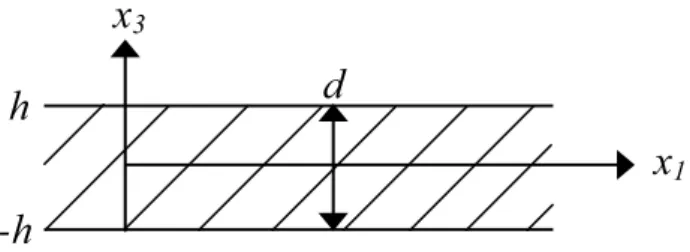
Figure 2.4: Schematic diagram of an innite plate in which the solution to the Lamb wave equation will be considered.

other than thickness, and is surrounded by vacuum. The innite extent of the plate allows edge eects and reections to be ignored, while the condition of existing in a vacuum ensures that there is no coupling between the plate and the surrounding medium, i.e.. that no energy is lost from the plate. The simple case considers a plane strain within the sheet, such that the complexity of the model can be reduced to two dimensions; x1, an innite dimension of the direction in which

the Lamb wave propagates, and x3, the nite dimension which represents the thickness of the

plate [38], as shown in gure 2.4. The assumption of a plane strain is valid where the width of the sheet in thex2direction is much larger than the wavelength of the Lamb waves, as is the case here. Under this assumption the wave equations for longitudinal and transverse waves given by equations 2.12 and 2.13 can be expressed as

∂2_φ

∂x2 1 +∂ 2_φ ∂x2 3 = 1 C2 L

∂2_φ

∂t2 (2.22)

∂2_ψ~ ∂x2 1

+∂ 2_ψ~ ∂x2 3

= 1

C2

T

∂2_ψ~

∂t2, (2.23)

where the velocities of the longitudinal and transverse waves are used in place of the Lamé parameters for simplicity. The solutions to these equations are assumed to consist of two separate components; a propagating wave travelling in the directionx1, of the formei(kx1−ωt), and a standing wave through the thickness of the sheet, described by the functions Φ (x3) and Ψ (x3) for the longitudinal and shear waves respectively [38, 97]. Combining these two components, the total wave equations in this case are,

φ = Φ (x3)ei(kx1−ωt) (2.24)

~ ψ

= Ψ (x3)e

(42)

The standing waves through the thickness of the sheet are often referred to as transverse resonance modes [38]. By substituting the proposed solutions into equations 2.22 and 2.23 the transverse resonance modes can be shown to have the form

Φ (x3) = A1sin(px3) +A2cos(px3) (2.26)

Ψ (x3) = B1sin(qx3) +B2cos(qx3) (2.27)

where the coecients A1, A2, B1 and B2 originate from solution of the partial dierential wave equations 2.22 and 2.23, andpandqare substitution variables dened as,

p2= ω 2

C2

L

−k2, q2= ω 2

C2

T

−k2. (2.28)

The particle displacement can be written in terms of the solutions to the standing modes through the thickness of the sheet, and by considering these particle displacements in conjunction with equation 2.6, the displacements and stresses are

u1 =

∂φ ∂x1

+ ∂ ~ψ

∂x3

=ikΦ + dΨ

dx3

, (2.29)

u3 =

∂φ ∂x3

− ∂ ~ψ

∂x1 = dΦ

dx3

−ikΨ, (2.30)

σ31 = µ

_∂u

3

∂x1 +∂u1

∂x3

=µ

2ikdΦ

dx3

+k2Ψ +d 2_Ψ

dx2 3

, (2.31)

σ33 = λ

∂u1

∂x1 +∂u3

∂x3

+ 2µ∂u3 ∂x3

=λ

−k2Φ +d 2_Φ

dx2 3

+ 2µ

d2Φ

dx2 3

−ikdΨ dx3

, (2.32)

where the factors ofik stem from the dierential of the x1 terms in the time varying component ofφandψ~,ei(kx1−ωt), and the exponential is omitted as it present in all of the equations.

The Lamb waves can be separated into two dierent regimes based on the symmetry of the wave about the centre of the plate, where the symmetry of the particle displacement in the plane of the plate, described by equation 2.29, is considered. For displacement in the plane the wave will be symmetric if the displacementu1contains only cosines, and antisymmetric if it contains only sines. This separation of the displacements and stresses into symmetric and antisymmetric components allows the solutions for the transverse resonance (equations 2.26 and 2.27) to be simplied such that Φ (x3) = A2cos(px3) and Ψ (x3) = B1sin(qx3) for the symmetric modes. From this the particle displacements and stresses of the symmetric modes can be written as [38,97],