Characterisation of damage in composite materials using infrared thermography

(1)

Master of Science Thesis

Characterisation of damage in composite

materials using infrared thermography

NLR

Royal Netherlands Aerospace Centre

UT

University of Twente

Author:

L.R. Kalter, BSc

University of Twente

Mechanical Engineering

[email protected]

Under supervision of:

Ir. J.S. Hwang

Netherlands Aerospace Centre - Aerospace Verhicles; Gas Turbines &

Structural Integrity

Dr. ir. D. Di Maio

University of Twente - Dynamics Based Maintenance

Prof. dr. ir. T. Tinga

University of Twente - Dynamics Based Maintenance

(2)

(3)

Acknowledgements

Before you lies the thesisCharacterisation of damage in composite materials using infrared thermog-raphy. This report is a thorough study into the characterisation capabilities of the different optical IR thermography methods. It is a result of my graduate internship at the Royal Netherlands Aerospace Center (NLR) in Marknesse. The report has been written to fulfil the graduation requirements of the master Mechanical Engineering at the University of Twente. I was engaged in conducting research and writing this thesis from February to September 2019.

This research is supported by the Royal Netherlands Aerospace Center (NLR). Founded in 1919 as

Rijksstudiedienst voor de luchtvaart (RSL), the goal of the NLR is to increase safety in aviation. While in 1919 the focus was on military aviation, the rapid upswing of civil aviation lead to the the widening of the NLR research [1]. The uprising of the modern computer resulted in new possibilities for the NLR, using all sorts of simulations for scientific research in the national aviation industry. In the twenty-first century, NLR focusses on making the aviation and aerospace industry more sustainable, safer and efficient.

I would like to thank my supervisors Dario di Mario and Tiedo Tinga from the University of Twente and Jason Hwang from the Royal Netherlands Aerospace Center for their support, availability and willingness to provide feedback and help with questions.

I would also like to thank Jacco Platenkamp and Arnoud Bosch for helping me with the experiments in the optical lab of the Aerospace Vehicles Test House. Lastly, I would like to thank my girlfriend for her support during my graduate internship.

L.R. Kalter, BSc

(4)

(5)

Abstract

The Non Destructive Testing (NDT) of large surface composite aerostructures is a very time consum-ing but critical process. Optical thermography is a relatively fast method for large surface inspection. This method is currently applied as first quick scan after which more detailed inspections are per-formed with different NDT methods to determine the defect properties and severity. This research is conducted to determine the defect characterisation capabilities of optical thermography as a NDT method for CFRP aerostructures.

In this research firstly, the current state of optical thermography methods is investigated. Two optical thermography methods have been tested experimentally and are investigated further using numerical simulations. Secondly, characteristics in the thermography results that can be used for the identification of the defect properties are identified. Thirdly, all factors that can influence the characteristics of the thermography results are determined. Experiments and numerical simulations are used to determine the sensitivity of the characteristics to these factors One-Factor-at-A-Time (OFAT). Finally, a window of possible values of the characteristics is obtained for three different defects; teflon coated glass, kap-ton and an air filled delamination. The obtained value windows can be used for defect characterisation.

The thermography methods are divided in two categories; frequency domain analysis thermography and pulse compression analysis thermography. The first applies Fast Fourier Transform (FFT) on the temperature signal of each pixel to obtain the phase at a certain frequency. The phase of a non defect area is then subtracted from the phase of a defect area to obtain the phase difference. This operation is performed for a range of frequencies resulting in the phase difference as a function of the frequency. Four characteristics are identified in this data; the peak phase difference, the peak phase frequency, the blind frequency and the phase transition frequency.

The second category applies Cross Correlation (CC) on the temperature signal of each pixel to obtain the cross correlation value as a function of the time delay. The difference in the normalized peak cross correlation value of the defect area and a non defect area is the first characteristic of this method. The second characteristic is the difference in time delay at which the correlation peak occurs for the defect and non defect area. The third characteristic is the cross correlation phase.

The influence of different heat signals, cameras and lamps on the characteristics is determined firstly after which the influence of the surface, the material and the defect are determined. This process is performed for both thermography method categories.

Two different NDT application scenarios are considered; in production and Maintenance Repair and Overhaul (MRO). In the composite production industry, the information on potential defects (foil and tape inclusions), the thickness and the properties of these materials are known. Even without detailed knowledge on the composite material properties, this makes characterisation of defects with optical thermography possible for the composite industry.

In the MRO industry, the knowledge on material properties of the composite is often limited. The type of sub surface defect expected in MRO inspections are delaminations of which the thickness can vary. However, characterisation of delaminations is possible with frequency domain thermography since the blind frequency characteristic is only marginally influenced by the air gap thickness. The thickness and depth of an air filled delamination can thus be determined within a range.

(6)

(7)

List of Figures

1.1 Percentage of aircraft mass comprised of composite materials (in initial configuration)

[5]. . . 1

1.2 Impact damage in composite structures, depending on the impact energy [10]. . . 2

2.1 The electromagnetic spectrum with the IR bandwidth [21]. . . 7

2.2 The absorbance of the electromagnetic radiation in the atmosphere [31]. . . 9

2.3 One dimensional thermal waves in a CFRP sample (kt= 0.7 W/mK,ρ= 1,528kg/m3, cp= 1,100 J/kgK) at a frequency of 0.1 Hz. . . 10

2.4 Schematic set-up of active thermography on a testobject with a subsurface defect. . . 11

2.5 Typical plot of the surface temperature decay of defect and non-defect regions after a pulse heat deposition.. . . 12

2.6 Schematic representation of the image processing of frequency domain analysis [39]. . . 13

2.7 Plots of the temperature over time with lock in thermography. . . 14

2.8 Phase difference between defective and non-defective area as a function of the excitation frequency with highlighted blind frequencyfb (simulated for NTP-A2 panel defect T3,1).. 15

2.9 Graphical explanation of Cross Correlation (CC). . . 16

2.10 The auto correlation of different signals with a length of 150 s. . . 16

2.11 Chirp signals (frequency from 0.5 Hz to 2.5 Hz in 10 sec). . . 18

2.12 Signals used for pulse compression. . . 18

3.1 Ishikawa diagram showing the influencing factors (in the boxes) and their parameters on thermography results. Green boxes indicate that the factors can be influenced by the set-up or the operator. Red boxes indicate that the factors can not be influenced.. . . 22

3.2 The experimental set-up.. . . 24

3.3 The solid CFRP panel samples. . . 25

3.4 The FEM mesh used in the simulations. The defect is highlighted with the red dashed line and the measurement locations with the 5 red dots.. . . 26

3.5 The steps in the data processing of frequency domain analysis.. . . 27

3.6 The steps in the data processing of pulse compression analysis. . . 28

4.1 Phase difference between defect and non defect regions of the coated surface at different LT frequencies, obtained with simulations and experiments. Two runs were performed with the experiment and four different reference regions are used as is shown in Figure 4.3a. 29 4.2 Phase difference between healthy and defect regions of the coated surface at different LT frequencies, obtained with simulations and experiments (Defect T1,1 on NTP-A2).. . . . 30

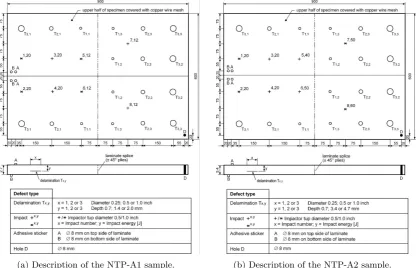
4.3 Experimental LT result at 0.3 Hz on the coated surface of the NTP-A2 sample (lower left quarter of the sample, cross like shape defects on the upper half of the image are impact damages). . . 30

4.4 Experimental LT result at 0.005 Hz showing the edge effect on the coated surface of the NTP-A2 sample (lower left quarter of the sample, cross like shape defects on the upper half of the image are impact damages).. . . 31

5.1 Frequency domain thermography simulation results of defect T3,1 of NTP-A2 (kl = 7 W/mK, kt= 0.7 W/mK ρ= 1,528 kg/m3 andcp = 1,100 J/kgK). . . 33

5.2 Temperature change of the NTP-A2 panel due to a 20 s pulse heat deposition as a function of the lamp power. . . 34

5.3 The surface temperature as a function of time for the defect T3,2 of NTP-A2 with kl = 7 W/mK and kt= 0.7 W/mK at three different heat flux with a frequency of 0.2 Hz and 6 cycles. . . 35

(10)

5.5 The surface temperature difference between defect region and non defect regions obtained from simulations with a 25.4 mm teflon coated glass insert at 1.4 mm depth with varying lamp power. . . 37 5.6 The phase difference for a 25.4 mm teflon coated glass insert at 0.7 mm and 1.4 mm

depth with 30µm and 115µm thick PU coating layer. . . 37 5.7 The phase difference as a function of the frequency for 25.4 mm teflon coated glass

inserts with varying out-of-plane thermal conductivitykt. . . 38

5.8 The phase difference as a function of the frequency for 25.4 mm teflon coated glass inserts with varying lateral thermal conductivitykl. . . 39

5.9 The phase difference as a function of the frequency for 25.4 mm teflon coated glass inserts. 39 5.10 The characteristics for 25.4 mm teflon coated glass inserts with varying thermal

diffu-sivityαtas a result of varying kt,ρandcp (the values ofαtcan be found in Table 5.3). 40

5.11 The characteristics for 25.4 mm teflon coated glass inserts with varying thermal diffu-sivityαtas a result of varying kt,ρandcp (the values ofαtcan be found in Table 5.3). 41

5.12 The peak phase difference for 25.4 mm teflon coated glass inserts varyingkt,cp andρ. . 42

5.13 Peak phase difference with different teflon coated glass defect sizes, depths and CFRP properties from Table 5.4. . . 43 5.14 The blind frequency with different teflon coated glass defect depths and the CFRP

prop-erties from Table 5.4. . . 43 5.15 The peak frequency with different teflon coated glass defect depths and the CFRP

prop-erties from Table 5.5. . . 44 5.16 The phase transition frequency with different teflon coated glass defect depths and the

CFRP properties from Table 5.5. . . 44 5.17 The phase difference as a function of the frequency for different defect sizes at different

depths. . . 45 5.18 The influence of the lateral size of a teflon coated glass insert on the characteristics. . . 46 5.19 Horizontal image shift of phase image with a frequency of 0.005 Hz. . . 46 5.20 The phase difference as a function of the frequency for different defect types and depths

and the material properties from Table 5.4. . . 47 5.21 The influence of the reflection coefficientR (and thus of the defect material and CFRP

material) and the defect depthdon the peak phase difference. The three coloured squares indicate the results regions for different defect materials and the four highlighted areas indicate the result regions for different defect depths. . . 48 5.22 The blind frequencyfbas a function of depth for the 5 scenarios from Table 5.4 and 5.5

for three different 25.4 mm defect materials (teflon, kapton and air) of 0.075 mm thick-ness. Combined with the theoretical (empirically determined) minimum and maximum. . 49 5.23 The peak phase difference as a function of the blind frequency fb for the 5 scenarios

from Table 5.4 and 5.5 for three different 25.4 mm defect materials (teflon, kapton and air) of 0.075 mm thickness at different depths (0.7 - 3.4 mm).. . . 49 5.24 Lock-in thermography simulation results with different defect thickness (thin = 37.5µm,

nom = 75µm and thick = 150µm). . . 50 6.1 Cross correlation of the reference signal and the temperature profile of a pixel in an

undamaged region of the NTP-A2 panel subjected to heat with a chirp signal of 1-0.01Hz (in 250s). . . 53 6.2 Experimental results of the linear chirp signal (1 - 0.01 Hz in 250 s) on the NTP-A2

sample. . . 55 6.3 The CC characteristics as a function of the defect depth for a 25.4 mm teflon coated

glass insert with the CFRP material properties from Table 6.8 and 6.9.. . . 58 6.4 The simulation results showing the CC characteristics for the three different defect

ma-terials (with a thickness of 75µm and a diameter of 25.4 mm) and the CFRP material properties from Table 6.8 and 6.9 as a function of the defect depth. . . 60 6.5 The normalised peak correlation value as a function of the CC phase with the regions

(11)

B.1 Image based technique illustrations. . . 76

C.1 The FLIR SC7600 on the camera stand. . . 77

D.1 Experimental results of the NTP-A2 sample with a linear chirp signal (0.5 - 0.05 Hz in 250 s). . . 79 D.2 Experimental results of the NTP-A2 sample with a quadratic chirp signal (0.5 - 0.05 Hz

in 250 s). . . 80 D.3 Experimental results of the NTP-A2 sample with a quadratic chirp signal (1 - 0.01 Hz

in 250 s). . . 81 D.4 Experimental results of the NTP-A2 sample with a 7-bit Barker code signal of 150 s. . . 82

E.1 The influence of the lateral heat conductionkl on FMTWI results for a 25.4 mm teflon

coated glass insert at different depths. . . 83 E.2 The influence of the out-of-plane thermal conductivity kt, the mass density ρ and the

thermal capacity cp on the thermography results for a 25.4mm diameter teflon coated

glass insert, as a function of the defect depth. . . 84 E.3 The influence of the through thickness conductivitykt, mass densityρand thermal

capac-itycpon the thermography results for a 25.4mm teflon coated glass insert, as a function

(12)

(13)

Nomenclature

Acronyms

2D Two Dimensional

3D Three Dimensional

ASTM American Society for Testing and Materials

AVTH Aerospace Vehicles Test House

BCTWI Barker Coded Thermal Wave Imaging

BVID Barely Visible Impact Damage

CC Cross Correlation

CFRP Carbon Fibre Reinforced Plastics

DFMTWI Digital Frequency Modulated Thermal Wave Imaging

DFT Discrete Fourier Transform

FEM Finite Element Method

FFT Fast Fourier Transform

FMTWI Frequency Modulated Thermal Wave Imaging

GFRP Glass Fibre Reinforced Plastics

IR Infrared Radiation

IRLT Infrared Radiation Lock-in Thermography

LT Lock-in Thermography

LWIR Long Wavelength Infrared Radiation

MRO Maintenance Repair and Overhaul

MWIR Medium Wavelength Infrared Radiation

NDE Non Destructive Evaluation

NDI Non Destructive Inspection

NDT Non Destructive Testing

NIR Near Infrared Radiation

NLR Royal Netherlands Aerospace Center

OFAT One-Factor-at-A-Time

POD Probability Of Detection

PPT Pulsed Phase Thermography

PSL Peak Sidelobe Level

(14)

QNDE Quantative Non Destructive Evaluation conference

RDID Readily Detectable Impact Damage

RGB Red Green Blue

SNR Signal to Noise Ratio

SWIR Short Wavelength Infrared Radiation

VLWIR Very Long Wavelength Infrared Radiation

Symbols

α Thermal diffusivity [m2/s]

λ Wavelength (of radiation) [m]

µ Penetration depth (or thermal diffusion length) [m]

φ Initial phase [rad]

ρ Mass density [kg/m3_]

σSB Stefan Boltzmann constant [Wm−2K−4]

T Total time [s]

τ Delay time [s]

ϕ Phase [deg]

A Amplitude [K]/[D.I.L.]/[a.u.]

B Calibrated distance between stereo cameras [m]

b Wien’s displacement constant [mK]

C Material correction factor [-]

C Volumetric heat capacity [J/m3_K]

c Loss of contrast [K]/[a.u.]

c1 First radiation constant [Wm2]

c2 Second radiation constant [mK]

cp Specific heat capacity (at constant pressure) [J/kgK]

d Defect depth [m]

e Thermal effusivity [J/s1/2_m2_K]

Eλ Spectral blackbody emissive power [W/m3]

f Focal length [m]

f0 Starting frequency [Hz]

f1 End frequency [Hz]

fb Blind frequency [Hz]

g(τ) Cross correlation [K2_s]/[(D.I.L.)2_s]/[a.u.]

(15)

h(t) Perceived thermal wave signal [K]/[D.I.L.]/[a.u.]

I(x, y, z, t) Rate of internal heat generation [W/m3_]

I0 Heat flux [W/m2]

k Thermal conductivity [W/mK]

kl Thermal conductivity in the lateral direction [W/mK]

kt Thermal conductivity in the through thickness direction[W/mK]

P(x, y, z) Position in three dimensions [m]

q Complex wave number [i/m]

R Reflection coefficient [-]

S(ω) Fourier transform of the reference signal [Ks]/[(D.I.L.)s]/[a.u.]

s(t) Reference signal [K]/[D.I.L.]/[a.u.]

Si Data point i [K]/[D.I.L.]/[a.u.]

T Absolute temperature [K]

t Time [s]

xi Position of camera i [m]

(16)

(17)

Chapter 1:

Introduction

In this chapter an introduction to the executed research is presented. To create an overview of testing for aerospace applications, section 1.1 presents an overview of damage types and Non Destructive Testing (NDT) methods for damage detection in the aerospace industry. Section 1.2 presents the scientific context of this research. Section 1.3 describes the objective of this thesis based on the scientific context and gaps in the knowledge on NDT. The objective is formulated in a research question in section 1.4. This chapter concludes with an outline of the remaining chapters in section 1.5.

1.1 Non Destructive Testing

Non destructive testing (NDT) can be described as a term for methods that are used to detect certain features in an object without changing the integrity or properties of the object irreversibly. In the field of aeronautical applications, the features sought after are defects, abnormalities or imperfections in components and structures [2].

In literature, the terms Non Destructive Investigation (NDI), Testing (NDT) and Evaluation (NDE) are commonly used as synonyms [3]. However, the three terms can be interpreted differently. NDI and NDT have an overlapping definition since both terms refer to qualitative measurements, but NDI is most commonly referred to for visual inspection methods. NDT is a wider term that includes the use of a range of different methods to test if an object has certain features. NDE is mostly referred to when the test results are quantitatively evaluated to determine characteristics of the detected features such as defect type, shape and depth. NDE also involves the making of the final judgement based on the test results. In the definition of NDT given by The American Society for Testing and Materials (ASTM), NDT also includes the evaluation of the test results: “NDT is the development and application of technical methods to examine materials or components in ways that do not impair future usefulness and serviceability in order to detect, locate, measure and evaluate discontinuities, defects and other imperfections; assess integrity, properties and composition; and measure geometrical characteristics.” [4]. In this report, it is chosen to use the term NDT as defined by the ASTM. The terms NDI and NDE will therefore not be used in this report.

NDT is an important part of the modern aviation and aerospace industry since it plays a crucial role in the safety of structures. One of the primary objectives of the aerospace industry is to increase fuel efficiency of aircrafts. To achieve this, weight reduction if one of the main design goals. This result in the trend of increasing application of Carbon and Glass Fibre Reinforced Polymers as can be seen in Figure 1.1 [5].

[image:17.595.181.418.580.737.2]

(18)

Composite materials consist of a matrix material with a reinforcing component. Composite materials are either constructed as solid laminate or a sandwich panel consisting of a low-density core material sandwiched between the two thin (1 - 2mm) panels [2]. The performance of fibre reinforced polymers is greatly influenced by abnormalities in the material. NDT methods are used to look for these ab-normalities in the material. Small defects can be acceptable depending on their nature and location. Depending on the size of the defect, it is decided whether or not to reject the object. The type of abnormalities that are potentially present in composite components is dependent on the life stage of the components. The component life can be divided in the production stage and the in-service stage. Aerospace structures are subject to extensive testing and evaluation during both production and the service life [2]. The most common defects obtained during production are resin-starved or resin-rich areas and cavities in the material as a result of entrapment of gasses or material inclusions such as Nylon or other tapes and foils [2].

Other types of defects occur during the service life of a component as a result of exposure to extreme environments, overloading and impact. The properties of composite materials are susceptible to degra-dation due to exposure to for example certain fluids, engine exhausts, fire and lightning strikes. The exposure to extreme environments may not be visible but can result in seriously degraded properties [2]. Overloading of a composite component may result in crack initiation or disbonding, while impacts cause different types of damage depending on the impact energy.

Composite materials are in general sensitive to impact [2]. Impacts can be caused by, for example, tool drops, flying debris on runways, bird strikes and hail storms. All of these cases result in different impact energies. Depending on the impact energy, impact damages range from easily identifiable holes in the surface to subsurface defects that are barely visible at the surface. In some cases the surface dent caused by low and medium energy impacts is visible directly after the damage is obtained but may become invisible over time [6]. The severity of the damage caused by an impact is dependent on the object shape and size, the impact energy, the laminate properties and thickness. Even a low energy impact (typically smaller than 40 J, see [7]) may result in fibre fracture, matrix cracking, delamination or disbonding of the sheet from the core material [2][8][9]. Although invisible from the outer surface, the internal damage can significantly influence the structural strength [2]. Medium energy impacts often result in a local surface dent with subsurface delaminations and fractures while high energy impacts can penetrate through the object creating a surface hole. The different types of impact damage in a solid laminate composite material are schematically shown in Figure 1.2.

(a)The type of damage. (b)The compression strength after impact.

Figure 1.2: Impact damage in composite structures, depending on the impact energy [10].

(19)

The critical size of discontinuities depends heavily on the function and design of the component [4]. Depending on the component and the critical defect type and size, a different NDT method can be applied. Several different methods are available for the testing and detection of defects, each method has its strengths and weaknesses, unfortunately there is no NDT method that is the best for all applications. The results of methods are sometimes combined resulting in a multi domain inspection method, more details on this can be found appendix A. The most commonly used NDT methods are listed below:

Visual inspection: Represents the first step of NDT examination. Has several advantages: simplicity, rapidity, low cost, minimal training and equipment requirements and the possibility to be performed while the part is being used or processed. However, the detection range is limited to the visible areas. Digital 3D scanners are also applied, more details on this technique can be found in appendix B.

Liquid penetrant: Makes use of a bright coloured fluid (the penetrant) that seeps into surface-breaking discontinuities. The visibility of these discontinuities is enhanced by the penetrant after removing the excess penetrant from the surface.

Electromagnetic methods: Uses electromagnetic sensors to detect disturbances caused by abnormalities in the object, in the magnetic field imposed on a conductive material.

Ultrasonic methods: Detects abnormalities based on the transmission or reflection of high frequency sonic waves (bandwidth 0.5-50 Mhz) through an object and measuring the amplitude, frequency and/or time of arrival of the returned echoes.

Thermography: Measures the surface temperatures of an object with an IR camera, combined with heat deposition on the object (active) or without heat deposition (passive). Disturbances in the heat flow caused by subsurface defects can be derived from the surface temperature over time.

Acoustic methods: Uses acoustic waves to detect defects. Ranges from the well-known ’coin-tap’ testing to acoustic resonance testing equipment.

Radiography: Makes use of radiation that is passed through an object and is projected onto a recoding medium to detect defects.

Shearography: Uses interference of laser speckle patterns to measure variations in the strain of the surface with cameras.

1.2 Research context

The inspection of aircraft components during and after manufacturing is a critical stage of the man-ufacturing process. Currently, ultrasonic NDT methods are mostly applied in production facilities to inspect the produced parts. This is a costly and time consuming process. On the other hand, airlines and the Maintenance Repair and Overhaul (MRO) industry have great interest in the automation and improvement of inspection methods for large surfaces to reduce both the planned ground time for periodic inspections and the unplanned ground time caused by for example impact damage.

(20)

The occurrence of certain events as a hail storm may result in the airplane being grounded for detailed impact damage inspection. The aircraft is visually inspected and detected damage is measured and evaluated. The administrative activities and more detailed checks required after visual inspection are labour-intensive. This results in very long inspection times (3-5 hours per square meter [15]). Visual inspection is limited to RDID and BVID while impact damage can cause subsurface damage that is not detectable with visual surface inspection. More detailed checks of suspected damage regions are there-fore required, this can for example be done using hand-held ultrasonic equipment. Since abnormalities greatly influence the structural integrity and thus the safety, early detection is of great importance. When an abnormality is detected, it can either be accepted when the safety is not compromised or considered a ’defect’ when the abnormality is not acceptable. The acceptance and rejection criteria are part of the damage tolerant design philosophy, this philosophy addresses the ability of components and structures to tolerate a certain density of specific damages while maintaining safe operation [4]. Both composite aircraft component manufacturers and the MRO industry are thus interested in fast and reliable inspection of composite parts.

The area of interest of this research is the effective inspection of large surfaces. Most NDT methods require contact with the test object while a contactless method is favourable for large surface inspec-tion since it requires less set-up time and no complicated mounting on the object is required. While most NDT methods focus on a relatively small area and small defects, both visual inspection and thermography are contact-less methods and both methods have the potential to be used to efficiently test large surface areas. These methods complement each other in the way that visual inspection is able to detect surface abnormalities while thermography is able to detect subsurface abnormalities. These methods are suitable for typical thin skin-stiffener aerospace structures.

The possibilities for combining computerized visual inspection and thermography have been investi-gated, see [16]. Computerized visual inspection can be used to detect defects with a surface dent or penetration. Three dimensional data acquisition is far evolved over the past two decades. Several techniques are available to effectively acquire a three-dimensional geometry. An overview of the recent developments in three dimensional data acquisition can be found in appendix B. Combining three dimensional data with thermography requires a lot of work to implement both methods efficiently. However, commercial software is available to map the two-dimensional thermography data on the three-dimensional geometry.

Thermography is an extensively researched field. Thermography is applied in numerous scientific fields including thermo-fluid dynamics, medicine, agriculture, building inspection, inspection of elec-trical components and NDT [17][18]. Thermography can be performed passively or actively with a heat source to actively deposit heat on the test object. Passive thermography is often applied to objects that generate heat internally such as electrical components. Aerospace structures often require an ex-ternal heat source to generate sufficient temperature differences. A collection of active thermography methods have been developed; Pulsed Thermography (PT), Pulsed Phase thermography (PPT), Lock in thermography (LT), Frequency Modulated Thermal Wave Imaging (FMTWI) and Barker Coded Thermal Wave imaging (BCTWI) [2][19][20]. The thermography methods differ in the type of signal used for the heat deposition and the processing method of the perceived temperature signal. This results in different depth ranges and detectability.

(21)

1.3 Research objective

Thermography is mainly applied as a quick method to locate subsurface defects, after which another NDT method such as ultrasonic scanning is used for defect characterisation. This characterisation consists of determining all the properties of the defect including the material, lateral size, thickness and depth location. The identified gap in thermography research is the characterisation of defects. Characterisation of defects with thermography enables the user to determine the nature and severity of a defect without having to apply other NDT methods on the sample.

The research objective is to determine the possibilities of using optical thermography to characterise defects in Carbon Fibre Reinforced Plastic (CFRP) aerostructures. This requires exploration of the characterisation capabilities of thermographic imaging techniques for both production and situ in-spection of composite aerospace structures.

As mentioned in section 1.1, the type of damages expected in a production and in-situ inspection are different. Also the environment and conditions under which these inspections are performed are different. The first types of defects are found in a controlled production environment while the second type of defects are found in the field during MRO inspection. Although both types of defects can occur within the same type of components, these types of defects are considered separately in this research since the conditions and knowledge on the inspected parts differ between the two environments.

1.4 Research questions

Based on the research objective described in section 1.3, the following main research question is for-mulated:

How and to what extend can damage in aerospace composite materials be characterised with the aid of optical thermography?

In order to answer this question, several subquestions have to be answered first, these questions are listed below:

What is the influence of the (partly unknown) composite material properties on the thermography results?

What is the influence of the different types of defects on the thermography results?

What is the influence of noise on the thermography results?

Which optical thermography method is the most conclusive in determining defect characters?

1.5 Research outline

(22)

(23)

Chapter 2:

Theory on thermography

This chapter aims to create a thorough overview of the knowledge relevant to this research. Optical thermography uses Infrared Radiation (IR) to determine the surface temperature. The physical theory of Infrared Radiation (IR) is described in section 2.1. Since only the surface temperature can be measured, the internal heat flow is important for subsurface defect detection. The heat flow in the test object can be described by thermal waves as is explained in section 2.2. The theory and recent advances in different optical thermography methods are described in section 2.3. This final section concludes with an overview of the advantages and disadvantages of the different thermography methods.

2.1 Infrared Radiation

Sir William Herschel discovered thermal radiation in the early 1800s, this discovery was first called Calorific Rays since the rays contained (thermal) energy. In the following two centuries, many other scientists (amongst them Macedonio Melloni, Gustav Kirchhoff, James Clerk Maxwell, Joseph Stefan, Ludwig Boltzmann, Max Planck)[18] worked on the theory of IR developing it into the knowledge of today.

Any object at a temperature above absolute zero emits electromagnetic radiation in the IR section of the electromagnetic spectrum. An overview of the electromagnetic spectrum is shown in Figure 2.1. The types of electromagnetic radiation can be classified by their wavelength in vacuum:

Short Wavelength Infrared Radation band (SWIR): from 0.76 to 2µm

Medium Wavelength Infrared Radiation Band (MWIR): from 2 to 4µm

Long Wavelength Infrared Radiation band (LWIR): from 4 to 14µm

Very Long Wavelength Infrared Radation band (VLWIR): from 14 to 1000µm

Figure 2.1: The electromagnetic spectrum with the IR bandwidth [21].

The spectral emittance of the electromagnetic radiationEλcan be described by Planck’s law in

Equa-tion 2.1 [22]. In Plank’s law,c1andc2are the first and second radiation constant,λis the wavelength

of the radiation and T is the absolute temperature of the black body.

Eλ=

c1

(24)

The maximum spectral radiance at a given temperature is given by Wien’s displacement law which is shown in Equation 2.2. In this equationbis the Wien’s displacement constant (≈2,898µm ·K).

λmax=

b

T (2.2)

Integration of Planck’s law over the entire spectrum results in the total hemispherical radiation intensity in Equation 2.3 in whichσSB is the Stefan-Boltzmann constant (≈5.67·10−8 W·m−2·K−4).

Eb=σSBT4 (2.3)

The equations stated above are applicable to blackbodies. Real objects are referred to as gray bodies since real objects only emit and absorb a fraction of this energy. The fraction of the emitted energy is called the emissivity of a material while the fraction of the incident flux that is absorbed by a object is called the absorbance. Next to the absorbed energy, a part of the energy is reflected. The emissivity, absorbance and reflectivity are dependent on the material, surface roughness and wavelength of the light [23].

Practical applications using the IR spectrum date back to the nineteenth century [24]. Many more ideas of IR applications are formed in the beginning of the twentieth century. Some of these appli-cations were detecting icebergs in 1914 [25] and monitoring forest fires in 1934 [26]. Appliappli-cations on material analysis started by measurements of thermophysical properties of materials. The basic idea of this technique dates back to 1937 by Vernotte who also described the effusivity of a material [27].

Effusivity is one of the material properties of importance in thermography as it describes the ability of a material to exchange thermal energy with its surroundings. The thermal effusivity is related to the thermal conductivityk, the mass density ρand the specific heat capacity cp as is described by

Equation 2.4.

e=pkρcp (2.4)

The first infrared camera was invented in 1929 for application in the anti-aircraft defence in Britain. In the 1940s the first thermographic camera in the form of infrared line scanners was developed by the U.S. military. This technique took one hour to produce a single image. It took until the 1960s for the first real-time thermographic camera to be commercially available, this type of camera used a cooled photoconductor [28]. A photoconductor directly detects photons and translates this into elec-trons. This results in either a current flow or a change in conductivity which is proportional to the radiance of the measured surface. This technique is still used for high-end cryogenic cooled cameras. A small Stirling cooler is used to keep the detector at a constant temperature of 77 K, resulting in a high sensitivity and less influence of stray radiation. Nowadays many different materials are applied in photoconductive detectors: amongst others PbSe, HdCdTe, InSb and PtSi [29]. In the 1990s, un-cooled microbolometer cameras became available on the commercial market, making IR technology more available and affordable [30]. In the recent years the detection frequency and resolution of IR cameras has improved rapidly [23].

IR cameras can detect Short Wave IR radiation (SWIR) or Long Wave IR radiation (LWIR). In the LWIR band, the absorbance of IR radiation by CO2 in the bandwidth of 4 to 4.5 µm and the

absorbance by H2O in the bandwith of 5.5 to 7.5 µm influences the measurements. The absorbance

(25)

Figure 2.2: The absorbance of the electromagnetic radiation in the atmosphere [31].

2.2 Thermal waves

Three dimensional heat flow in a solid object is the basis of the indirect measurements performed with thermography. The three dimensional heat flow in a solid object can be described by the parabolic diffusion equation given in Equation 2.5.

∂ ∂x

kx

∂ T(x, y, z, t) ∂x + ∂ ∂y ky

∂ T(x, y, z, t) ∂y + ∂ ∂z kz

∂ T(x, y, z, t) ∂z

+I(x, y, z, t) =C∂ T(x, y, z, t) ∂t

(2.5) In this equationki is the thermal conductivity in direction i, I(x, y, z, t) is the rate of internal heat

generation, which is zero for structural components and C is the volumetric heat capacity of the object. The equation can be simplified if we assume an isotropic homogeneous semi-infinite solid object, resulting in the one dimensional out-of-plane heat transfer described by Equation 2.6.

∂2_T

∂x2 −

1 α

∂T

∂t = 0 (2.6)

In this equation α is the thermal diffusivity and equals the ratio between the thermal conductivity k and the heat capacity C. The thermal diffusivity is a measure for the rate of transfer of heat in a material from hot to cold regions. The assumption of an isotropic homogeneous semi-infinite solid object is not valid for composite material samples. The one dimensional approach does however provide insight in the behaviour of heat flow. By assuming the only heat flow with the surrounding of the sample is described by the boundary condition in Equation 2.7 which describes the heat deposited on the top surface by a frequency modulated heat source, one can obtain the temperature distribution within the solid.

−k∂ T(x, t) ∂x

_x₌₀

= I0 2Re

h

(1 + exp(iωt))i (2.7)

The heat deposition on the top surface consists of two factors. The first factor is the time independent temperature rise, described by the first term in the square brackets of Equation 2.7. The second factor is the periodic temperature oscillation described by the second term in the brackets of Equation 2.7. As will be explained in section 2.3, the term of interest for most thermography methods is the pe-riodic temperature oscillation. “The temperature oscillations resulting from the periodical heating of the surface, can be described by thermal waves. Thermal waves are often described as the solution of the parabolic heat diffusion equation (Equation 2.6) in the presence of a periodical time varying heat source modulated in intensity at a given frequency. ” [32]

Equation 2.6 can be solved for the periodic oscillating boundary condition by substitution of Equa-tion 2.8 resulting in EquaEqua-tion 2.9 [33][34][35].

(26)

∂2_θ(x)

∂x2 −q

2_{θ(x) = 0} _(2.9)

In this equation,qis the complex wave vector given by Equation 2.10.

q= 1 +i

µ (2.10)

In this equation, the penetration depthµ is the distance over which heat is transported in the sam-ple during one modulation cycle. The penetration depth (or thermal diffusion length) is inversely proportional to the modulation frequency as is described by Equation 2.11.

µ=

r _α

πf (2.11)

From the relation between the penetration depth µ and the frequency f of the heat deposition in Equation 2.11, it can be concluded that lower frequencies penetrate deeper in the sample material. From Equation 2.9, the following solution for the temperature distribution can be derived [35]:

T(x, t) = I0 2e√ω exp

−x µ cos _x

µ+ωt+ π 4

(2.12)

This solution is a highly damped plane wave propagating in the x-direction. The heat flow in an object resulting from periodically oscillating energy deposition can thus be described as highly damped plane waves, although it is not an actual wave equation since it does not have the second-order time deriva-tive of a wave equation. An example of the thermal waves in a CFRP sample subject to periodical heating can be seen in Figure 2.3.

Figure 2.3: One dimensional thermal waves in a CFRP sample (kt = 0.7 W/mK, ρ= 1,528 kg/m3,

cp= 1,100 J/kgK) at a frequency of 0.1 Hz.

The thermal wave propagates in this manner until an interface is reached. At an interface, thermal waves are reflected and refracted. To solve the temperature distribution over an interface, the tem-perature and heat flux must be consistent at the interface. Taking the continuity of the temtem-perature and heat flux as boundary condition at the interface, the reflection coefficientRof the thermal waves travelling from material 1 to material 2 in Equation 2.13 is obtained [33][34][35].

R12=

e1−e2

e1+e2

=

p

k1ρ1cp1−

p

k2ρ2cp2

p

k1ρ1cp1+pk2ρ2cp2

(2.13)

(27)

2.3 Thermography techniques

Thermography is the measurement of the surface temperature of an object using an IR camera that detects IR and produces images of the radiation intensity. Thermography methods can be split in two categories, active and passive methods. In passive methods, no external excitation is applied while in active methods an external excitation is applied in the form of a heating or cooling source. Although both active and passive thermography are applied in the field of NDT, active thermography is more common [23]. Passive thermography is often applied to objects that generate heat internally, for ex-ample the detection of hot spots on integrated circuit boards [2]. The lack of temperature differences in defects in composite materials results in a low sensitivity for defects with passive thermography, thus limiting the application for damage detection [2]. However, active thermography is frequently applied in damage detection in composite materials since an external energy source is used to increase the temperature, enlarging the difference between the defect and non defect regions. Commonly used methods for excitation are optical and ultrasound. In this report the focus is put on optical excitation since this method is better applicable to large surfaces. The schematic set-up of an active optical thermography method can be seen in Figure 2.4.

Figure 2.4: Schematic set-up of active thermography on a testobject with a subsurface defect.

Local differences in the surface temperature can be caused by several factors including both exter-nal and interexter-nal factors. The exterexter-nal factors can be considered disturbances to the thermography process since the accuracy of the method is decreased by these influences. The external factors that can influence the surface temperature are amongst others, the heating source, humidity and air flow. The internal factors are related to the heat flow of the material. The heat flow is affected by internal features of the material. Next to the thermal properties of the material, these features can be different kind of abnormalities; delaminations, moisture ingress, spurious material inclusions, resin rich regions or fibre distortions, but also the geometry of the object.

The disadvantage of thermography is the limited depth-penetration capability of the technique. The maximum detectable defect depth is dependent on the thermal properties of the material. Defects in GFRP for example are proven to be detectable up to 6 mm [36], but detectability is highly dependent on the defect size, defect thickness and the thermal properties of both the defect and the sample material. For other materials a larger depth can be inspected depending on the thermal properties of the material.

Multiple methods of active optical thermography are applied in the NDT field [2][19][20].

Pulsed Thermography(PT): A widely applied method, the reason for the popularity of PT is the short inspection time. The method relies on a short thermal excitation in the form of pulsation of a high power flash lamp. The analysis is done in the time domain.

Pulsed Phase Thermography (PPT): Uses a pulse signal from high power flash lamps. The analysis is done in the frequency domain to obtain the amplitude and phase.

(28)

Frequency Modulated Thermal Wave Imaging (FMTWI): Uses a chirp signal to deposit heat over a longer time period spread over multiple frequencies. The analysis can either be done in the frequency domain or by applying Cross Correlation (CC).

Barker Coded Thermal Wave Imaging (BCTWI): Uses a 7-bit Barker code signal to deposit heat. This signal is specially developed for the application in CC.

[image:28.595.203.392.559.719.2]

These method differ in signal used for heat deposition on the surface and in the way the perceived signal is analysed. Since some of these methods use either the same signal or the same signal processing method, an overview of the methods is given in Table 2.1.

Table 2.1: Overview of the heat source, heat signal and data processing method of the different optical thermography methods.

Method Heat source Heat signal Data processing method

PT Flash lamp(s) (Dirac) pulse Time domain

PPT Flash lamp(s) (Dirac) pulse Frequency domain (FFT)

LT Lamp(s) / laser Sine wave Frequency domain (FFT/Lock-in)

FMTWI Lamp(s) / laser Chirp Frequency domain (FFT)/Pulse compression (CC)

BCTWI Lamp(s) / laser 7-bit Barker code Pulse compression (CC)

These methods have been studied extensively over the past 20 years by a large group of scientists. The different methods are split based on the data processing method used since this determines the results of the thermography methods. The application of time domain analysis, frequency domain analysis (using lock-in/FFT) and pulse compression analysis (using Cross Correlation (CC)) in thermography are explained in the subsection 2.3.1, 2.3.2 and 2.3.3 respectively. In each of these subsections the suitable heat sources and heat signals for each type of analysis are also discussed. Lastly, subsection 2.3.4 summarizes the differences of the thermography methods.

2.3.1 Time domain analysis

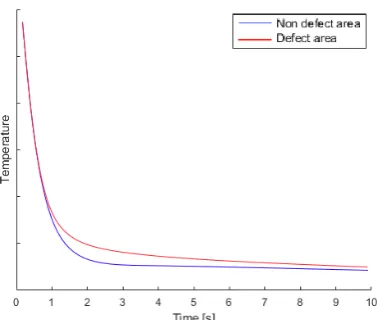
The analysis in the time domain relies on a short thermal excitation in the form of a pulsation from a high power flash lamp. The lamp deploys heat to the surface of the object for a duration of a few milliseconds. After the heating period the surface temperature is measured with an IR camera to obtain the temperature decay curve. The temperature decay of the front surface is caused by propa-gation of the thermal wave front, radiation at the surface and convection at the surface. Subsurface abnormalities influence the propagation of heat inside the material resulting in a different surface tem-perature above the abnormality with respect to non defect regions as can be seen in the typical surface temperature decay curve in Figure 2.5.

(29)

Since the detection of abnormalities is dependent on the thermal propagation in the material, deeper defects are observed later than shallow defects. The deeper defects have a reduced contrast due to the attenuation of the thermal wave in the depth direction and the lateral heat dissipation. The observation timet and the contrastc are be described by Equation 2.14 and 2.15 respectively [23].

t≈ d

2

α (2.14)

c≈ 1

d3 (2.15)

In these equations,dis the defect depth andαis the thermal diffusivity. Time domain analysis (Pulse Thermography) is very sensitive to variations of test conditions [2]. Uneven heating or reflection on the surface influences the surface temperature distribution and thus directly influence the results. This limits the applicability of the method to controllable environments in which even distribution of the heat source over the surface is possible.

2.3.2 Frequency domain analysis

The temperature of the surface is measured during the heating process using an IR camera. This time-domain data can be transferred to the frequency domain by using a lock-in amplifier or by using a Discrete Fourier transformation (DFT) from Equation 2.16 for each pixel separately [2][37][38].

Fn= N−1

X

k=0

T(k)e−2πikn/N = Ren+iImn (2.16)

After transferring the data to the frequency domain, the amplitude A and phase ϕcan be obtained for each pixelnusing Equation 2.17 and 2.18 respectively.

An=

q

Re2_n+ Im2_n (2.17)

ϕn = tan−1

_Im

n

Ren

(2.18)

[image:29.595.214.382.541.659.2]

By analysing the data for each pixel separately, amplitude and phase images are obtained as is schemat-ically shown in Figure 2.6. The amplitude image is sensitive to inhomogeneities of the test surface, the emissivity and the distribution of the applied heat [2]. In the phase image, each of these effects is eliminated by processing the data on pixel level [2]. This is very useful for practical applications of thermography in aerospace industry since the surfaces are curved and large, making uniform heating very hard to achieve.

Figure 2.6: Schematic representation of the image processing of frequency domain analysis [39].

(30)

Three different heat signals can be used for frequency domain analysis in thermography, the first is a pulse signal, the second is a periodical sine wave signal and the third is a linear chirp signal. Using a pulse signal in combination with frequency analysis is referred to as Pulsed Phase Thermography (PPT). Using a sine wave in combination with frequency domain analysis is called Lock-in Thermog-raphy (LT) and lastly the combination of a linear chirp signal with frequency domain analysis is called Frequency Modulated Thermal Wave Imaging (FMTWI). Each of the three methods is explained in more detail.

Pulsed Phase Thermography (PPT) uses a pulse signal (similar to PT) for the energy deposition on the test object surface. An ideal pulse of null duration has a frequency spectrum with uniform energy distribution over all frequencies. Real pulses have a finite duration and amplitude, the signal contains different energy at different frequencies. The energy distribution over frequencies is determined by the pulse duration, longer pulses concentrate energy in lower frequencies. The inspection of deeper regions requires lower frequencies as is clear from Equation 2.11, thus the pulse duration must be increased. This spreads the available energy over the frequencies resulting in lower energy at high frequencies and thus increased influence of noise at these frequencies [2]. The available energy is limited due to the short period of time heat is applied to the surface and the maximum power of the source. For accurate testing at different depths, multiple measurements with varying pulse lengths must be performed [2].

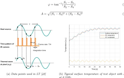
Lock in Thermography (LT) uses a sinusoidal power modulation of the heat source to deposit heat on the test object surface. The heat is applied using an optical source, in most cases one (or multiple) halogen lamp(s). In some cases a laser is used as a heating source. The temperature modulation results in a periodical transfer of heat to the surface. The heat propagates into the test object as a thermal wave. Since the signal is a sine-wave, the phaseϕand amplitudeAcan also be found by using the four-point algorithm using Equation 2.19 and 2.20 respectively. Using more four-points reduces the influence of the noise. In these equations, S1 toS4 are equidistant signal data points as shown in Figure 2.7a.

Practical heat sources are however unable to cool the object, resulting in an increasing global trend of the surface temperature. The sample is heated for several cycles until a near equilibrium DC temperature has been reached as can be seen in Figure 2.7b. A multiple (1-10) of cycles are measured after the DC temperature has reached an equilibrium to obtain accurate results using Equation 2.19 and 2.20. This results in a cycle time of several minutes for lower frequencies. An alternative method is de-trending the signal to obtain the AC component.

ϕ= tan−1(S1−S3 S2−S4

) (2.19)

A=p(S1−S3)2+ (S2−S4)2 (2.20)

[image:30.595.99.498.475.726.2]

(a)Data points used in LT [40] (b) Typical surface temperature of test object with LT at 0.25Hz

(31)

For the LT analysis, the energy is concentrated around the frequency of the excitation source whilst a pulse contains a broader frequency spectrum. This increases the contrast with respect to PPT where the limited energy is spread over a range of frequencies. For Carbon Fibre Reinforced Plastic (CFRP) materials, the excitation frequency is normally within the range from approximately 0.001 Hz - 5 Hz [41][42]. For high conductive materials like metals, higher frequencies are commonly used in the range up to 50 Hz [43].

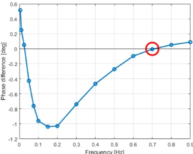
All defects have a blind frequency fb, which is a frequency at which the defect region has no phase

shift with respect to non defect regions and the defect can thus not be identified using the phase data. For frequencies above the blind frequency, the phase difference is small and approaches zero with increasing frequency. A plot of the phase shift for different excitation frequencies is shown in Figure 2.8, in this plot the blind frequency is highlighted with a red circle. Theoretically the blind frequency can be predicted when the material properties, defect depth and location are known [44][45]. Experiments by several authors suggests that the blind frequency correlates to 1.5 to larger than 2 times the penetration depth at that frequency [46][47][48]. This can be described by Equation 2.21.

d=Cµ=C

r_α

t

πfb

(2.21)

In this equationCis the material correction factor (1.5 to 2+),dis the defect depth,αtis the thermal

diffusivity and fb is the blind frequency. In practical NDT applications, the propertiesC and αt are

[image:31.595.200.393.375.529.2]

not exactly known. It is therefore necessary to always test on multiple frequencies resulting in long measurement times. This is one of the main limitations of LT and led to the application of a chirp signal.

Figure 2.8: Phase difference between defective and non-defective area as a function of the excitation frequency with highlighted blind frequencyfb (simulated for NTP-A2 panel defect T3,1).

Frequency Modulated Thermal Waves Imaging (FMTWI) uses a chirp signal with which the surface heating is done with a range of frequencies. This range of frequencies can be chosen based on the test subject and its properties. The signal is a low peak-power, long duration modulated wave signal. The linear chirp signal is described in time by Equation 2.22 and is shown in Figure 2.11a.

s(t) =Acos

2π

f1−f0

2T t+f0

t+φ

(2.22)

In Equation 2.22A is the amplitude of the signal, f0 is the start frequency, f1 is the end frequency,

T is the total signal time and φ is the initial phase. The advantage of using a linear chirp signal is that a range of frequencies is covered, the phase can thus be determined for multiple frequencies using the data from one measurement. This requires significantly less measurement time and only a single measurement to obtain the data in Figure 2.8 for a defect [49].

(32)

2.3.3 Pulse compression analysis

In the search for higher sensitivity and resolution, using pulse compression is proposed as processing method [50]. Pulse compression is a technique that is often used in radar systems since it is designed to enhance the detection sensitivity, resolution and reduce noise. The cross correlation g(τ) of the reference signals(t) and the perceived signal h(t) can be determined by Equation 2.23 or 2.24. The first is in the time domain while the latter is in the frequency domain.

g(τ) =

Z ∞

−∞

s(t)h(τ+t)dt (2.23)

g(τ)∝ F−1_[S(ω)_∗_H(ω)] _(2.24)

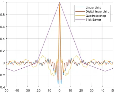
As an explanatory example, the Cross Correlation (CC) of a sine signal and a cosine signal is shown in Figure 2.9. With increasing time delayτ, the red cosine signal is shifted to the right resulting in different values for the correlation. The resulting correlation value is shown in Figure 2.9b. Since these signals are periodical in nature, the cross-correlation is also periodical. The period of the signals is set to 2 s, the time shift between the sine and cosine signal is thus 0.5 s. This results in a peak in the cross correlation at a delay time of 0.5 and 2.5 s. The length of the signals is limited, resulting in a value of zero if the time delayτ is larger than the duration of the reference signals(t). Non-periodical signals are more suitable for CC since these signals have one cross correlation peak instead of a periodical peak value as can be seen in Figure 2.10.

(a) Sine signal with a length of 6 s and a cosine signal with a length of 2 s.

[image:32.595.204.391.560.714.2]

(b) The Cross Correlation of the signals in Fig-ure 2.9a.

Figure 2.9: Graphical explanation of Cross Correlation (CC).

(33)

The time delay and value of the cross correlation main peak are the characteristics that can be deter-mined for each pixel resulting in a peak correlation image and a peak delay image respectively. The time delay of the main peak is determined using Equation 2.25.

τCCpeak =τ|{g(τ)=max(g(τ))} (2.25)

The CC peak value is dependent on the magnitude of both the perceived signalh(t) and the reference signal s(t). The amplitude of the reference signal can be set to one. However, the amplitude of the measured signal is directly dependent on the heat distribution on the surface. Uneven heating therefore greatly influences the CC peak value. In 2011, Tabatabaei et al. suggested the cross correlation phase as a method to normalize the CC peak value [51]. The cross correlation phase can be obtained by dividing the cross correlation of the signal and the reference by the cross correlation of the signal and the quadrature of the reference as is shown in Equation 2.26. The quadrature of the reference signal is determined by performing a Hilbert transform which is the term between square brackets in the denominator of Equation 2.26.

ϕCC =

F−1_(S(ω)_∗_H_(ω))

F−1_([₋_i_{sgn(ω)S(ω)]}_∗_H_(ω))

_τ₌₀

(2.26)

Both the time shift, the magnitude of the CC peak and the CC phase can be a measurement of the defect depth [50][51]. In recent years, several experiments have been conducted on CC as analysis method for thermography, all showing the improved Signal to Noise Ratio (SNR) in comparison with LT [52][53][54]. Applications have expanded to concrete inspection [55] and human breast cancer in-spection [56].

All non periodical signals are in theory suitable for pulse compression using CC. However there are several signals which result in a good Peak Sidelobe Level (PSL). The Peak Sidelobe Level (PSL) can be determined using Equation 2.27.

PSL = 20 log(Side lobe peak

Main lobe peak) dB (2.27)

Several signals have been applied in thermography:

Linear chirp signal (Figure 2.11a)

Digital chirp signal (Figure 2.11b)

Quadratic chirp signal (Figure 2.12a)

7-bit Barker signal (Figure 2.12b)

(34)

The result of the quadratic chirp and the 7-bit Barker code signals on the correlation function is shown in Figure 2.10. The reduced PSL in theory results in a higher SNR leading to a high contrast between defective and non-defective regions [59][61].

Many efforts have been put into the use of a Barker sequence codes in NDT over the past 10 years [20][52]. In 2018, Fei Wang et al. used a truncated-correlation of a pulsed chirp signal with a laser heat source for qualitative three-dimensional visualization of surface cracks by changing the reference signal delay time [62]. BCTWI has been applied to CFRP and GFRP materials, verifying the detectability of defects with this method and the superiority of the method in comparison with LT [20][52][53][63][64]. However no effort has been done to link the thermography results to defect characters and further research is required on this subject.

(a)Linear chirp signal (b)Digital chirp signal

Figure 2.11: Chirp signals (frequency from 0.5 Hz to 2.5 Hz in 10 sec).

(a)Quadratic up chirp signal (b)7 bit Barker signal

(35)

2.3.4 Comparison of the optical thermography methods

As discussed in the previous subsections, different methods are available for optical IR thermography. The methods differ in the heat source and the heat signal used for the heat deposition and the process-ing method for the measurement data. An overview of these differences has been provided in Table 2.1.

Due to the fundamental differences between the methods, the results obtained also differ. PT and PPT deposit heat on the object using a pulse signal. PT is sensitive to uneven heating and reflections of the surface making it unsuitable for large surface in-situ inspections. PPT is less sensitive to these factors since the phase is analysed for each pixel separately. PPT is however limited in the amount of heat that can be deposited on the surface due to the pulse length. Both PT and PPT require very high powered lamps in order to deposit enough heat on the surface in a few millisecond duration flash.

Frequency domain analysis with a sine wave or a chirp signal spreads the energy deposition over a longer time. The long duration low peak power heat deposition makes deeper defects detection pos-sible without overheating the object and with only a limited peak power required from the lamps. The pulse compression analysis also uses low peak power long duration signals, but these signals are processed using CC resulting in different thermography results. The pulse compression analysis results in a higher SNR than the frequency domain analysis.

(36)

(37)

Chapter 3:

Methodology

This chapter elaborates on the methodology used in this research in order to answer the research question. The research question (see section 1.4) is split in four sub questions. The sub questions are repeated here for the convenience of the reader:

What is the influence of the (partly unknown) composite material properties on the thermography results?

What is the influence of the different types of defects on the thermography results?

What is the influence of noise on the thermography results?

Which optical thermography method is the most conclusive in determining defect characters?

Thermography is a secondary method, meaning that the method does not directly measure defect properties but only the temperature of the top surface. From this temperature, different results are obtained depending on the thermography method. Therefore the results and characteristics of each method must be determined. From these results, relevant features need to be determined regarding the subsurface defect. Due to secondary nature of the thermography measurement, several factors influence the results. An overview of these factors and their parameters is shown in section 3.1. In this section, the method for determining the influence of each factors is discussed.

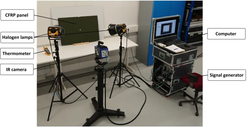
The samples available for this research are limited to a single CFRP material and teflon coated glass inserts as is discussed in section 3.2. The samples are not sufficient to answer the first and second research question. Numerical simulations are therefore used to vary the properties of influence to the thermography results. The experiments are used to validate the simulation model and determine the influence of noise on the thermography results. In section 3.2 details on the experimental set-up and the CFRP samples used in this research are provided.

Numerical simulations are used to vary properties, such as the thermal conductivity of the material, that are difficult to vary in real samples. Section 3.3 shows the details of the simulation model. The simulations are used to determine the sensitivity of the process to different properties and provide insight in how the techniques work under ideal circumstances without noise. The data obtained from both the simulations and the experiments require processing. The data processing method differs for the different thermography methods. The data processing in the frequency domain analysis and the pulse compression analysis are discussed in section 3.4.

To provide an answer to the last question, the steps above are executed for the frequency domain analysis and the pulse compression analysis and processed separately in chapter 5 and 6 respectively. Conclusions to each of the questions stated above are formulated in chapter 7.

3.1 Influencing factors and their parameters

(38)

Figure 3.1: Ishikawa diagram showing the influencing factors (in the boxes) and their parameters on thermography results. Green boxes indicate that the factors can be influenced by the set-up or the operator. Red boxes indicate that the factors can not be influenced.

It is clear that the thermography results are not only influenced by the properties of the defect. In order to characterize defects with the thermography results, either the value of the parameters or the sensitivity of the results to the parameters in Figure 3.1 needs to be known. Since often not all parameters are known, the sensitivity of the results to the parameters is determined using a One-Factor-at-A-Time (OFAT) analysis. This type of analysis determines the influence of several factors one at a time instead of testing the influence of multiple factors simultaneously. This provides a clear view of the influence of each parameter. However, the interaction between the influence of different factors is not included in an OFAT analysis. This is overcome by combining the influence of each of the parameters to obtain a set of parameters that result in the boundary values for the thermography results. The parameters will be elaborated here for each factor, starting with the factors in the green boxes from Figure 3.1 and ending with the factors in the red boxes.

Thermography method This research focusses on two signal processing methods as is discussed in subsection 2.3.4. The different data processing methods generate different results. Frequency domain analysis provides a phase and amplitude value for each pixel at different modulation frequencies. Pulse compression analysis results in a peak correlation value, peak delay time and cross correlation phase for each pixel. The characteristics of these signals are determined and the sensitivity of these characteristics to variations in all other parameters is obtained by varying the parameters one at a time. Since different signals can be used for both methods, the difference in heat signals is also a parameter that can influence the thermography results.

Lamps The halogen lamps can vary the process in several ways; the total power, the distance from the surface and the angle towards the surface. The result of varying these parameters is a different heat flux at the surface of the sample. As a 5 W heat flux does not result in a significant temperature increase while a 50 kW heat flux would result in overheating the component and damaging it, the total heat flux can influence the detectability of defects and the results. The amount of heat absorbed by the sample is measured and the sensitivity of the results to variations of this heat flux are determined by increasing and decreasing the lamp power in both experiments and numerical simulations.

Camera The camera used for the thermography measurements has an effect on the detectability of defects. The sample rate of the camera directly determines the amount of data obtained by the measurement. The processing of the data is limited to this discrete step size. The detection bandwidth and thermal and spatial resolution limit the detectability of defects. These limitations are taken into account in the comparison of the simulations and the experiments.

Characterisation of damage in composite materials using infrared thermography

Master of Science Thesis