warwick.ac.uk/lib-publications
Original citation:Iglesias, Marco, Lu, Yulong and Stuart, Andrew M.. (2016) A Bayesian level set method for geometric inverse problems. Interfaces and Free Boundaries, 18 (2). pp. 181-217.
Permanent WRAP URL:
http://wrap.warwick.ac.uk/86351
Copyright and reuse:
The Warwick Research Archive Portal (WRAP) makes this work by researchers of the University of Warwick available open access under the following conditions. Copyright © and all moral rights to the version of the paper presented here belong to the individual author(s) and/or other copyright owners. To the extent reasonable and practicable the material made available in WRAP has been checked for eligibility before being made available.
Copies of full items can be used for personal research or study, educational, or not-for-profit purposes without prior permission or charge. Provided that the authors, title and full
bibliographic details are credited, a hyperlink and/or URL is given for the original metadata page and the content is not changed in any way.
Publisher’s statement:
Originally published in Interfaces and Free Boundaries 2016 http://dx.doi.org/10.4171/IFB/362
A note on versions:
The version presented here may differ from the published version or, version of record, if you wish to cite this item you are advised to consult the publisher’s version. Please see the ‘permanent WRAP URL’ above for details on accessing the published version and note that access may require a subscription.
for Geometric Inverse Problems
Marco A. Iglesias
†, Yulong Lu
∗and Andrew M. Stuart
‡
†
School of Mathematical Sciences, University of Nottingham, Nottingham NG7 2RD, UK
∗
Mathematics Institute, University of Warwick, Coventry CV4 7AL, UK
‡
Mathematics Institute, University of Warwick, Coventry CV4 7AL, UK
∗
corresponding author. [email protected]
Abstract
We introduce a level set based approach to Bayesian geometric inverse problems. In these problems the interface between different domains is the key unknown, and is realized as the level set of a function. This function itself becomes the object of the inference. Whilst the level set methodology has been widely used for the solution of geometric inverse problems, the Bayesian formulation that we develop here contains two significant advances: firstly it leads to a well-posed inverse problem in which the posterior distribution is Lipschitz with respect to the observed data; and secondly it leads to computationally expedient algorithms in which the level set itself is updated implicitly via the MCMC methodology applied to the level set function – no explicit velocity field is required for the level set interface. Applications are numerous and include medical imaging, modelling of subsurface formations and the inverse source problem; our theory is illustrated with computational results involving the last two applications.
1
Introduction
Geometric inverse problems, in which the interfaces between different domains are the primary un-known quantities, are ubiquitous in applications including medical imaging problems such as EIT [9] and subsurface flow [5]; they also have an intrinsically interesting mathematical structure [30]. In many such applications the data is sparse, so that the problem is severely under-determined, and noisy. For both these reasons the Bayesian approach to the inverse problem is attractive as the proba-bilistic formulation allows for regularization of the under-determined, and often ill-posed, inversion via the introduction of priors, and simultaneously deals with the presence of noise in the observa-tions [32, 45]. The level set method has been a highly successful methodology for the solution of classical, non-statistical, inverse problems for interfaces since the seminal paper of Santosa [43]; see for example [15, 11,12, 47,33, 34,46, 13,18, 19,48, 28,3, 6] and for related Bayesian level set approaches see [49,36,37,40].
1
In this paper we marry the level set approach with the Bayesian approach to geometric inverse problems. This leads to two significant advances: firstly it leads to a well-posed inverse problem in which the posterior distribution is Lipschitz with respect to the observed data, in the Hellinger metric – there is no analogous well-posedness theory for classical level set inversion; and secondly it leads to computationally expedient algorithms in which the interfaces are updated implicitly via the Markov chain Monte Carlo (MCMC) methodology applied to the level set function – no ex-plicit velocity field is required for the level set interface. We highlight that the recent paper [48] demonstrates the potential for working with regularized data misfit minimization in terms of a level set function, but is non-Bayesian in its treatment of the problem, using instead simulated annealing within an optimization framework. On the other hand the paper [49] adopts a Bayesian approach and employs the level set method, but requires a velocity field for propagation of the interface and does not have the conceptual and implementational simplicity, as well as the underlying theoretical basis, of the method introduced here. The papers [36, 37, 40], whilst motivated by the Bayesian approach, use the ensemble Kalman filter and are therefore not strictly Bayesian – the method does not deliver a provably reliable approximation of the posterior distribution except for linear Gaussian inverse problems.
The key idea which underpins our work is this. Both the theory and computational practice of the level set method for geometric inverse problems is potentially hampered by the fact that the mapping from the space of the level set function to the physical parameter space is discontinuous. This discontinuity occurs when the level set function is flat at the critical levels, and in particular where the desired level set has non-zero Lebesgue measure. This is dealt with in various ad hoc
ways in the applied literature. The beauty of the Bayesian approach is that, with the right choice of prior in level set space, these discontinuities have probability zero. As a result a well-posedness theory (the posterior is Lipschitz in the data) follows automatically, and computational algorithms such as MCMC may be formulated in level set space. We thus have practical algorithms which are simultaneously founded on a sound theoretical bedrock.
2
Bayesian Level Set Inversion
2.1
The Inverse Problem
This paper is concerned with inverse problems of the following type: recover functionκ ∈ X :=
Lq(D;
R), D a bounded open set in R2, from a finite set of noisily observed linear functionals
{Oj}Jj=1ofp∈V, for some Banach spaceV, wherep=G(u)for nonlinear operatorG∈C(X, V).
Typically, for us,κwill represent input data for a partial differential equation (PDE),pthe solution of the PDE andGthe solution operator mapping the inputκto the solutionp. Collecting the linear functionals into a single operatorO :V →RJ and assuming additive noiseηwe obtain the inverse
problem of findingκfromywhere
y= (O ◦G)(κ) +η. (2.1)
This under-determined inverse problem is well-adapted to both the classical [20] and Bayesian [17] approaches to regularized inversion, becauseO ◦G∈C(X,RJ).
2.2
Level Set Parameterization
There are many inverse problems whereκis knowna priorito have the form
κ(x) =
n
X
i=1
κiIDi(x); (2.2)
here ID denotes the indicator function of subset B ⊂ R2, {Di}ni=1 are subsets of D such that
∪n
i=1Di = D and Di ∩ Dj = ∅, and the {κi}ni=1 are known positive constants.1 In this setting
theDi become the primary unknowns and the level set method is natural. Given integer n fix the
constantsci ∈Rfori= 0,· · · , nwith−∞=c0 < c1 <· · ·< cn=∞and consider a real-valued
continuouslevel set functionu:D→R. We can then define theDi by
Di ={x∈D|ci−1 ≤u(x)< ci}. (2.3)
It follows that Di ∩ Dj = ∅ for i, j ≥ 1, i 6= j. For later use define the i-th level set Di0 =
Di∩Di+1 ={x∈D|u(x) =ci}. LetU =C(D;R)and, given the positive constants{κi}ni=1, we
define the level set mapF :U →X by
(F u)(x)→κ(x) =
n
X
i=1
κiIDi(x). (2.4)
We may now defineG =O ◦G◦F :U →RJ and reformulate the inverse problem in terms of the
level set functionu: findufromywhere
y=G(u) +η. (2.5)
1Generalization to theκ
ibeing unknown constants, or unknown smooth functions on each domainDi, are possible
However, becauseF : U → X, and hence G : U → RJ, is discontinuous, the classical
regular-ization theory for this form of inverse problem is problematic. Whilst the current state of the art for Bayesian regularization assumes continuity ofGfor inverse problems of the form (2.5), we will demonstrate that the Bayesian setting can be generalized to level set inversion. This will be achieved by a careful understanding of the discontinuity set forF, and an understanding of probability mea-sures for which this set is a measure zero event.
2.3
Well-Posed Bayesian Inverse Problem
In the Bayesian approach to inverse problems, all quantities in (2.5) are treated as random variables. LetU denote a separable Banach space and define a complete2 probability space(U,Σ, µ0)for the
unknown u. (In our applications U will be the space C(D;R) but we state our main theorem in more generality). Assume that the noise η is a random draw from the centered Gaussian Q0 := N(0,Γ); we also assume that η and u are independent.3 We may now define the joint random variable(u, y) ∈U ×RJ. The Bayesian approach to the inverse problem (2.5) consists of seeking
the posterior probability distribution µy of the random variable u|y, u given y. This measure µy
describes our probabilistic knowledge about uon the basis of the measurements y given by (2.5) and the prior informationµ0onu.
We define theleast squares functionΦ :U ×RJ →
R+by
Φ(u;y) = 1
2|y− G(u)|
2
Γ (2.6)
with| · | := |Γ−12 · |.We now state a set of assumptions under which the posterior distribution is
well-defined via its density with respect to the prior distribution, and is Lipschitz in the Hellinger metric, with respect to datay.
Assumptions 2.1. The least squares functionΦ : U ×RJ →
Rand probability measureµ0 on the
measure space(U,Σ)satisfy the following properties:
1. for everyr >0there is aK =K(r)such that, for allu∈U and ally∈RJ with|y| Γ< r,
0≤Φ(u;y)≤K;
2. for any fixed y ∈ RJ, Φ(·;y) : U →
R, is continuous µ0-almost surely on the complete
probability space(U,Σ, µ0);
3. fory1, y2 ∈RJ withmax{|y1|Γ,|y2|Γ}< r, there exists aC=C(r)such that, for allu∈U,
|Φ(u;y1)−Φ(u;y2)| ≤C|y1−y2|Γ.
2Complete probability space is defined at the start of Appendix 2
3Allowing for non-Gaussianη is also possible, as is dependence betweenη andu; however we elect to keep the
The Hellinger distance betweenµandµ0is defined as
dHell(µ, µ0) =
1 2 Z U r dµ dν −
r dµ0
dν !2 dν 1 2
for any measureνwith respect to which µandµ0 are absolutely continuous; the Hellinger distance is, however, independent of which reference measureνis chosen. We have the following:
Theorem 2.2. Assume that the least squares functionΦ :U×RJ →
Rand the probability measure
µ0 on the measure space (U,Σ) satisfy Assumptions 2.1. Then µy µ0 with Radon-Nikodym
derivative
dµy dµ0
= 1
Z exp(−Φ(u;y)) (2.7)
whera, foryalmost surely,
Z :=
Z
U
exp(−Φ(u;y))µ0(du)>0.
Furthermoreµy is locally Lipschitz with respect to y, in the Hellinger distance: for ally, y0 with
max{|y|Γ,|y0|Γ}< r, there exists aC =C(r)>0such that
dHell(µy, µy
0
)≤C|y−y0|Γ.
This implies that, for allf ∈L2
µ0(U;S)for separable Banach spaceS,
kEµyf(u)−Eµy
0
f(u)kS ≤C|y−y0|.
Remarks 2.3. • The interpretation of this result is very natural, linking the Bayesian picture
with least squares minimisation: the posterior measure is large on sets where the least squares function is small, and vice-versa, all measured relative to the priorµ0.
• The key technical advance in this theorem over existing theories overviewed in [17] is that
Φ(·;y) is only continuous µ0−almost surely; existing theories typically use that Φ(·;y) is
continuous everywhere on U and that µ0(U) = 1; these existing theories cannot be used
in the level set inverse problem, because of discontinuities in the level set map. Once the technical Lemma6.1has been established, which usesµ0−almost sure continuity to establish
measurability, theproofof the theorem is a straightforward application of existing theory; we therefore defer it to Appendix 1.
• What needs to be done to apply this theorem in our level set context is to identify the sets of discontinuity for the mapG, and hence Φ(·;y), and then construct prior measures µ0 for
• Theconsequencesof this result are wide-ranging, and we name the two primary ones: firstly we may apply the mesh-independent MCMC methods overviewed in [16] to sample the poste-rior distribution efficiently; and secondly the well-posedness gives desirable robustness which may be used to estimate the effect of other perturbations, such as approximatingGby a nu-merical method, on the posterior distribution [17].
2.4
Discontinuity Sets of
F
We return to the specific setting of the level set inverse problem whereU =C(D;R). We first note that the level set mapF :U → L∞(D;R)is not continuous except at pointsu ∈U where no level crossings occur in an open neighbourhood. However as a mappingF :U → Lq(D;
R)forq < ∞
the situation is much better:
Proposition 2.4. For u ∈ C(D) and 1 ≤ q < ∞, the level set map F : C(D) → Lq(D) is
continuous atuif and only ifm(Di0) = 0for alli= 1,· · ·, n−1.
The proof is given in Appendix 1. For the inverse gravimetry problem considered in the next section the spaceXis naturallyL2(D;
R)and we will be able to directly use the preceding
proposi-tion to establish almost sure continuity ofF and henceG. For the groundwater flow inverse problem the spaceX is naturallyL∞(D;R)and we will not be able to use the proposition in this space to establish almost sure continuity ofF. However, we employ recent Lipschitz continuity results for GonLq(D;R),q <∞to establish the almost sure continuity ofG[8].
2.5
Prior Gaussian Measures
LetDdenote a bounded open subset ofR2. For our applications we will use the following two con-structions of Gaussian prior measuresµ0 which are GaussianN(0,Ci), i= 1,2on Hilbert function
spaceHi, i= 1,2.
• N(0,C1)on
H1 :={u:D→R|u∈L2(D;R)),
Z
D
u(x)dx= 0},
where
C1 =A−α and A :=−∆ (2.8)
with domain4
D(A) :={u:D→R|u∈H2(D;R),∇u·ν = 0on∂Dand Z
D
u(x)dx= 0}.
• N(0,C2)onH2 :=L2(D;R)withC2 :H2 → H2being the integral operator
C2φ(x) =
Z
D
c(x, y)φ(y)dy withc(x, y) = exp
−|x−y|
2
L2
(2.9)
In fact, in the inverse model arising from groundwater flow studied in [26,25], the Gaussian measure
N(0,C1)was taken as the prior measure for the logarithm of the permeability. On the other hand the
Gaussian measureN(0,C2)is widely used to model the earth’s subsurface [39] as draws from this
measure generate smooth random functions in which the parameterL sets the spatial correlation length. For both of these measures it is known that, under suitable conditions on the domain D, draws are almost surely inC(D;R); see [17], Theorems 2.16 and 2.18 for details.
Assume that α > 1 in (2.8), then the Gaussian random function with measure µ0 defined in
either case above has the property that, for U := C(D;R), µ0(U) = 1. Since U is a separable
Banach spaceµ0 can be redefined as a Gaussian measure onU. Furthermore it is possible to define
the appropriateσ-algebraΣin such a way that(U,Σ, µ0)is a complete probability space; for details
see Appendix 2. We have the following, which is a subset of what is proved in Proposition7.2.
Proposition 2.5. Consider a random functionudrawn from one of the Gaussian probability
mea-suresµ0onU given above. Thenm(Di0) = 0, µ0-almost surely, fori= 1,· · · , n.
This, combined with Proposition2.4, is the key to making a rigorous well-posed formulation of Bayesian level set inversion. Together the results show that priors may be constructed for which the problematic discontinuities in the level set map are probability zero events. In the next section we demonstrate how the theory may be applied, by consider two examples.
3
Examples
3.1
Test Model 1 (Inverse Potential Problem)
LetD⊂R2 be a bounded open set with Lipschitz boundary. Consider the PDE
∆p=κ inD, p= 0 on∂D. (3.1)
Ifκ∈X :=L2(D)it follows that there is a unique solutionp∈H1
0(D). Furthermore∆p∈L2(D),
so that the Neumann trace can be defined inV :=H−12(∂D)by the following Green’s formula:
D∂p ∂ν, ϕ
E
∂D =
Z
D
∆pϕdx+
Z
D
∇p∇ϕdx
for ϕ ∈ H1(D). Here ν is the unit outward normal vector on ∂D and h·,·i
∂D denotes the dual
pairing on the boundary. We can then define the bounded linear mapG:X →V byG(κ) = ∂ν∂p. Now assume that the source termκhas the form
for some D1 ⊆ D. The inverse potential problem is to reconstruct the supportD1 from
measure-ments of the Neumann data ofp on∂D. In the case where the Neumann data is measured every-where on the boundary∂D, and where the domainD1 is assumed to be star-shaped with respect to
its center of gravity, the inverse problem has a unique solution; see [30,31] for details of this theory and see [23, 13] for discussion of numerical methods for this inverse problem. We will study the underdetermined case where a finite set of bounded linear functionalsOj : V → Rare measured,
noisily, on∂D:
yj =Oj
∂p ∂ν
+ηj. (3.2)
Concatenating we havey= (O ◦G)(κ) +η.Representing the boundary ofD1as the zero level set
of functionu∈U :=C(D;R)we write the inverse problem in the form (2.5):
y= (O ◦G◦F)(u) +η. (3.3)
Since multiplicity and uncertainty of solutions are then natural, we will adopt a Bayesian approach. Notice that the level set map F : U → X is bounded: for all u ∈ U we have kF(u)kX ≤
Vol(D) := RDdx. SinceG : X → V andO : V → RJ are bounded linear maps it follows that G = O ◦ G◦F : U → RJ is bounded: we have constant C+ ∈
R+ such that, for allu ∈ U,
|G(u)| ≤C+.From this fact Assumptions2.1(i) and (iii) follow automatically. Since bothG:X →
V andO : V → RJ are bounded, and hence continuous, linear maps, the discontinuity set of G
is determined by the the discontinuity set ofF : U → X.By Proposition 2.4this is precisely the set of functions for which the measure of the level set{u(x) = 0}is zero. By Proposition2.5 this occurs with probability zero for both of the Gaussian priors specified there and hence Assumptions
2.1(ii) holds with these priors. Thus Theorem2.2applies and we have a well-posed Bayesian inverse problem for the level set function.
3.2
Test Model 2 (Discontinuity Detection in Groundwater Flow)
Consider the single-phase Darcy-flow model given by
− ∇ ·(κ∇p) =f inD, p= 0 on∂D. (3.4)
HereDis a bounded Lipschitz domain inR2,κthe real-valued isotropic permeability function and
p the fluid pressure. The right hand sidef accounts for the source of groundwater recharge. Let V = H01(D;R), X = L∞(D;R)andV∗ denote the dual space ofV. Iff ∈ V∗ andX+ := {κ ∈
X : essinfx∈Dκ(x) ≥ κmin > 0}thenG : X+ 7→V defined byG(κ) = pis Lipschitz continuous
and
kG(κ)kV =kpkV ≤ kfkV∗/κmin. (3.5)
characterize heterogeneous subsurface structure in a physically meaningful way. We thus have
κ(x) =
n
X
i=1
κiIDi(x)
where{Di}ni=1 are subsets ofDsuch that∪ni=1Di = DandDi∩Dj = ∅, and where the{κi}ni=1
are positive constants. We letκmin = miniκi.
Unique reconstruction of the permeability in some situations is possible if the pressurepis mea-sured everywhere [2, 41]. The inverse problem of interest to us is to locate the discontinuity set of the permeability from a finite set of measurements of the pressurep. Such problems have also been studied in the literature. For instance, the paper [46] considers the problem by using multiple level set methods in the framework of optimization; and in [27], the authors adopt a Bayesian approach to reconstruct the permeability function characterized by layered or channelized structures whose ge-ometry can be parameterized finite dimensionally. As we consider a finite set of noisy measurements of the pressurep, inV∗, and the problem is underdetermined and uncertain, the Bayesian approach is again natural. We make the significant extension of [27] to consider arbitrary interfaces, requiring infinite dimensional parameterization: we introduce a level set parameterization of the domainsDi,
as in (2.3) and (2.4).
LetO :V →RJ denote the collection ofJlinear functionals onV which are our measurements.
Because of the estimate (3.5) it is straightforward to see thatG =O ◦G◦F is bounded as a mapping fromU intoRJ and hence that Assumptions2.1(i) and (iii) hold; it remains to establish (ii). To that
end, from now on we need slightly higher regularity onf. In particular, we assume that, for some q > 2, f ∈ W−1(Lq(D)). Here the space W−1(Lq(D)) := (W01,q∗(D))∗ ⊂ V∗ for q∗ and q conjugate:1/q+ 1/q∗ = 1. It is shown in [8] that there exitsq0 >2such that the solution of (3.4)
satisfies
k∇pkLq(D)≤CkfkW−1(Lq(D))
for someC <∞ provided2 ≤ q < q0. We assume that such aq is chosen. It then follows thatG
is Lipschitz continuous fromLrtoV wherer := 2q/(q−2) ∈[2,∞). To be precise, letp
i be the
solution to the problem (3.4) withκi, i= 1,2. Then the following is proved in [8]: for anyq ≥2,
kp1−p2kV ≤
1
κmin
k∇p1kLq(D)kκ1−κ2kLr(D)
provided∇p1 ∈Lq(D).
Hence G : Lr(D) → V is Lipschitz under our assumption that f ∈ W−1(Lq(D)) for some
q ∈ (2,0). . By viewing F : U → Lr(D), it follows from Proposition (2.4) and Proposition
4
Numerical Experiments
Application of the theory developed in subsection 2.3 ensures that, for the choices of Gaussian priors discussed in subsection2.5, the posterior measure on the level set is well defined and thus suitable for numerical interrogation. In this section we display numerical experiments where we characterize the posterior measure by means of sampling with MCMC. In concrete we apply the preconditioned Crank-Nicolson (pCN) MCMC method explained in [16]. We start by defining this algorithm. Assume that we have a prior Gaussian measureN(0,C)on the level set functionuand a posterior measureµy given by (2.7). Define
a(u, v) = min{1,exp Φ(u)−Φ(v)}
and generate{u(k)}
k≥0as follows:
Algorithm 4.1(pCN-MCMC).
Setk = 0and picku(0) ∈X
1. Proposev(k) =p
(1−β2)u(k)+βξ(k), ξ(k) ∼ N(0,C).
2. Setu(k+1) =v(k) with probabilitya(u(k), v(k)), independently of(u(k), ξ(k)).
3. Setu(k+1) =u(k)otherwise.
4. k→k+ 1and return to (i).
Then the resulting Markov chain is reversible with respect to µy and, provided it is ergodic,
satisfies
1
K
K
X
k=0
ϕ u(k)
→Eµy
ϕ(u)
for a suitable class of test functions. Furthermore a central limit theorem determines the fluctuations around the limit, which are asymptotically of sizeK−12.
4.1
Aim of the experiments
source term of the PDE (3.1) given data/observations from the solution of this PDE. Similarly, given data/observations from the solution of the Darcy flow model (3.4), we wish to estimate the inter-face between geologic facies{Di}ni=1 corresponding to regions of different structural geology and
which leads to a discontinuous permeabilityκ(x) =Pn
i=1κiIDi(x)in the flow model (3.4). In both
test models, we introduce the level set function merely as an artifact to parameterize the unknown geometry (i.e. Di ={x∈D|ci−1 ≤u(x)< ci}), or equivalently, the resulting discontinuous field
κ(x). The Bayesian framework applied to this level/ set parameterization then provides us with a posterior measureµy on the level set functionu. The push-forward ofµy under the level set mapF
(2.4) results in a distribution on the discontinuous field of interestκ. This push-forward of the level set posteriorF∗µy :=µy◦F−1 comprises the statistical solution of the inverse problem which may,
in turn, be used for practical applications.
A secondary aim of the experiments is to explore the role of the choice of prior on the posterior. Because the prior is placed on the level set function, and not on the model paramerers of direct interest, this is a non-trivial question. To be concrete, the posterior depends on the Gaussian prior that we put on the level set. While the prior may incorporate our a priori knowledge concerning the regularity and the spatial correlation of the unknown geometry (or alternatively, the regions of discontinuities in the fields of interest) it is clear that such selection of the prior on the level set may have a strong effect on the resulting posteriorµy and the corresponding push-forwardF∗µy. One of
the key aspects of the subsequent numerical study is to understand the role of the selection of the prior on the level set functions in terms of the quality and efficiency of the solution to the Bayesian inverse problem as expressed via the push-forward of the posteriorF∗µy.
4.2
Implementational aspects
For the numerical examples of this section we consider synthetic experiments. The PDEs that define the forward models of subsection3(i.e. expressions (3.1) and (3.4)) are solved numerically, on the unit-square, with cell-centered finite differences [4]. In order to avoid inverse crimes [32], for the generation of synthetic data we use a much finer grid (size specified below) than the one of size
80×80used for the inversion via the MCMC method displayed in Algorithm4.1.
The Algorithm4.1 requires, in step (i), sampling of the prior. This is accomplished by param-eterizing the level set function in terms of the Karhunen-Loeve (KL) expansion associated to the prior covariance operatorC (See Appendix 2, equation (7.1)). Upon discretization, the number of eigenvectors ofC equals the dimensions of the discretized physical domain of the model problems (i.e.N = 6400in expression (7.2)). Once the eigendecomposition ofC has been conducted, then sampling from the prior can be done simply by sampling an i.i.d set of random variables{ξk}with
ξ1 ∼ N(0,1)and using it in (7.2). For the present experiments we consider all these KL modes
car-ried out on the full set of KL modes. This mechanism enables the MCMC method to quickly reach an “optimal” state where the samples of the level set function provides a fieldκ(x)that is close to the truth. However, once this optimal state has been reached, it is essential to conduct the sampling on the full spectrum of KL modes to ensure that the MCMC chain mixes properly. More precisely, if only the lowest modes are retained for the full chain, the MCMC may collapse into the optimal state but without mixing. Thus, while the lowest KL modes determine the main geometric structure of the underlying discontinuous field, the highest modes are essential for the proper mixing and thus the proper and efficient characterization of the posterior.
4.3
Inverse Potential Problem
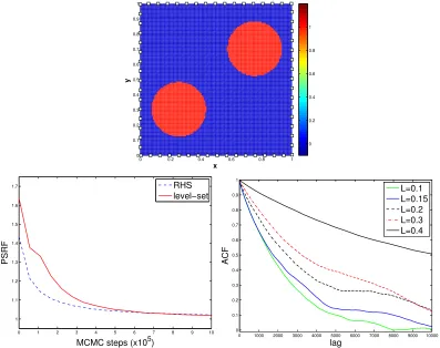
In this experiment we generate synthetic data by solving (3.1), on a fine grid of size 240×240
with the “true” indicator function κ† = ID†
1 displayed in Figure Figure 1 (top). The observation
operatorO = (O1, . . . ,O64)is defined in terms of 64 mollified Dirac deltas{Oj}64j=1 centered at
the measurement locations display as white squares along the boundary of the domain in Figure1
(top). Each coordinate of the data is computed by means of (3.3) withpfrom the solution of the PDE with the aforementioned true source term and by adding Gaussian noiseηj with standard deviation
of 10% of the size of the noise-free measurements (i.e. of Oj(∂p∂ν)). We reiterate that, in order to
avoid inverse crimes [32], we use a coarser grid of size80×80for the inversion via the MCMC method (Algorithm4.1). The parameterization ofD1 in terms of the level set function is given by
D1 ={x∈D|u(x)<0}(i.e. by simply choosingc0 =−∞andc1 = 0in (2.3)).
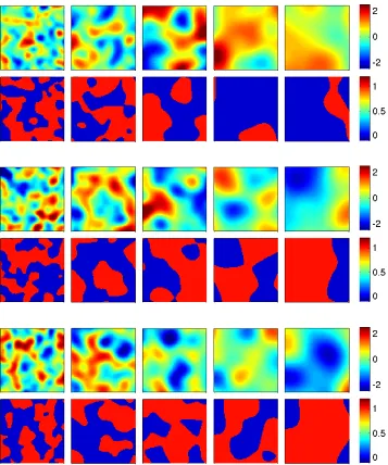
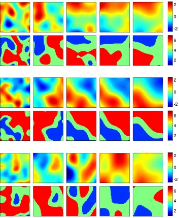
For this example we consider a prior covarianceCof the form presented in (2.9) for some choices ofLin the correlation function. We constructC directly from this correlation function and then we conduct the eigendecomposition needed for the KL expansion and thus for sampling the prior. In Figure2we display samples from the priorN(0,C)on the level set functionu(first, third and fifth rows) and the corresponding indicator functionκ = ID1 (second, fourth and sixth rows) for (from
left to right)L = 0.1,0.15,0.2,0.3,0.4. Different values of L in (2.9) clearly result in substantial differences in the spatial correlation of the zero level set associated to the samples of the level set function. The spatial correlation of the zero level set funtion, under the prior, has significant effect on
ID1 which we use as the right-hand side (RHS) in problem (3.1) and whose solution, via expression
(3.3), determines the likelihood (2.6). It then comes as no surprise that the posterior measure on the level set is also strong;y dependent on the choice of the prior via the parameterL. We explore this effect in the following paragraphs.
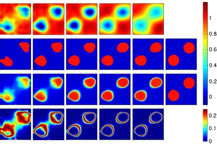
In Figure3 we present the numerical results from different MCMC chains computed with dif-ferent priors corresponding to the aforementioned choices of L. The MCMC mean of the level set function is displayed in the top row of Figure 3 for the choices (from left to right) L = 0.1,0.15,0.2,0.3,0.4. We reiterate that although the MCMC method provides the characterization of the posterior of the level set function, our primary aim is to identify the fieldκ(x) =ID1(x)that
A straightforward estimate of such field can be obtained by mapping, via the level set map (2.4), the posterior mean level set function denoted byuinto the corresponding fieldF(u(x)) = κ(x) =
ID1(x)whereD1 ={x∈D|u(x)<0}. We displayκ(x) =ID1(x)in the top-middle row of Figure 3along with the plot of the true fieldκ† =ID†
1 (right column) for comparison.
As mentioned earlier, we are additionally interested in the push-forward of the posterior measure of the level set function u under the level set map (i.e. (F∗µy)(du)). We characterize F∗µy by
mapping underF our MCMC samples from µy. In Figure3we present the mean (bottom-middle)
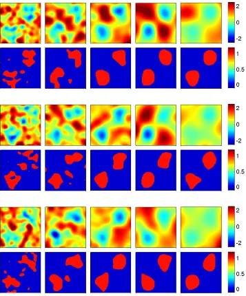
and the variance (bottom) of F∗µy. Figure 4 shows some posterior (MCMC) samples u of the level set function (first, third and fifth rows) and the corresponding level set mapF(u) = ID1 with
D1 ={x∈D|u(x)<0}associated to these posterior samples (second, fourth and sixth rows).
The push-forward of the posterior measure under the level set map (i.e. F∗µy) thus provides
a probabilistic description of the inverse problem of identifying the true κ† = ID†
1. We can see
from Figure3that, for some choices ofL, the mean ofF∗µy provides reasonable estimates of the
truth. However, the main advantage of the Bayesian approach proposed here is that a measure of the uncertainty of such estimate is also obtained from F∗µy. The variance (Figure 3 bottom), for
example, is a measure of the uncertainty in the location of the interface between the two regionsD andD\D1.
The results displayed in Figure3show the strong effect that the selection of the prior has on the posterior measureµy and the corresponding pushforward measureF∗µy. In particular, there seems
to be a critical valueL = 0.2above of which the corresponding posterior mean onF∗µy provides
a reasonable identification of the trueID†
1 with relatively small variance. This critical value seems
to be related to the size and the shape of the inclusions that determines the true regionD†1 (Figure
1(top)). It is intuitive that posterior samples that result from very small spatial correlation cannot easily characterize these inclusions accurately unless the data is overwhelmingly informative. The lack of a proper characterization of the geometry from priors associated with smallLis also reflected with larger variance around the interface. It is then clear that the capability of the proposed level set Bayesian framework to properly identify a shapeD1†(or alternatively its indicator functionID†
1)
depends on properly incorporating, via the prior measure, a priori information on the regularity and spatial correlation of the unknown geometry ofD1†.
method produces samples that are highly correlated and thus very long chains may be needed in order to produce a reasonable number of uncorrelated samples needed for statistical analysis. For this particular choice ofL= 0.3we have conducted 50 multiple MCMC chains of length106(after
burn-in period) initialized from random samples from the prior. In Figure1(bottom-left) we show the Potential Scale Reduction Factor (PSRF) [10] computed from MCMC samples of the level set function (red-solid line) and the corresponding samples underF (i.e. theID1’s) (blue-dotted line).
We observe that the PSRF goes below 1.1 after (often taken as an approximate indication of conver-gence [10]); thus the Gelman-Rubin diagnostic [10] based on the PSRF is passed for this selection ofL. The generation of multiple independent MCMC chains that are statistically consistent opens up the possibility of using high-performance computing to enhance our capabilities of properly ex-ploring the posterior. While we use a relatively small number of chains as a proof-of-concept, the MCMC chains are fully independent and so the computational cost of running multiple chains scales with the number of available processors.
The5×107 samples that we obtained from the50 MCMC chains are combined to provide a full characterization of the posteriorµy on the level set and the corresponding push-forwardF∗µy
(i.e. TheID1’s computed from D1 with posterior samplesu). We reemphasize that our aim is the
statistical identification ofI†D
1. Therefore, in order to obtain a quantity from the true ID†1 against
to which compare the computed push-forward of the level set posterior, we consider the Discrete Cosine Transform (DCT) of the true field ID. Other representations/expansions of the true field
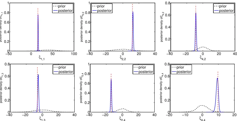
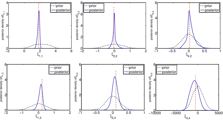
could be considered for the sake of assessing the uncertainty of our estimates with respect to the truth. In Figure 5 we show the prior and posterior densities of the first DCT coefficients of ID1
where D1 = {x ∈ D |u(x) < 0} with u from our MCMC samples (the vertical dotted line
corresponds to the DCT coefficient of the trueID†
1). We can observe how the push forward posterior
0 0.2 0.4 0.6 0.8 1 0 0.1 0.2 0.3 0.4 0.5 0.6 0.7 0.8 0.9 1 x y 0 0.2 0.4 0.6 0.8 1
0 1 2 3 4 5 6 7 8 9 10
1 1.1 1.2 1.3 1.4 1.5 1.6 1.7
MCMC steps (x105)
PSRF
RHS level−set
[image:16.612.97.494.229.543.2]0 1000 2000 3000 4000 5000 6000 7000 8000 9000 10000 0 0.1 0.2 0.3 0.4 0.5 0.6 0.7 0.8 0.9 1 lag ACF L=0.1 L=0.15 L=0.2 L=0.3 L=0.4
Figure 1: Inverse Potential. Top: True source termκ† = ID†
1 of eq. (3.1). Bottom-left: PSRF from
Figure 2: Inverse Potential. Samples from the prior on the level set functionu(first, third and fifth rows) for (from left to right) L = 0.1,0.15,0.2,0.3,0.4. Corresponding ID1 with D1 = {x ∈
Figure 3: Inverse Potential. MCMC results for (from left to right)L = 0.1,0.15,0.2,0.3,0.4in the eq. (2.9). Top: Posterior mean level set functionu(computed via MCMC). Top-middle: Plot ofID1 withD1 = {x ∈ D|u(x) < 0}(the truth ID†1 is presented in the right column). Bottom-middle:
Mean ofID1 where D1 ={x∈ D|u(x)< 0}andu’s are the posterior MCMC samples (the truth
is presented in the right column). Bottom: Variance ofID1 where D1 = {x ∈ D |u(x) < 0}and
−500 0 50 100 0.2 0.4 0.6 0.8 1 ξ 1,1
posterior density of
ξ1,1
prior posterior
−400 −20 0 20 40
0.2 0.4 0.6 0.8 1 ξ 2,2
posterior density of
ξ2,2
prior posterior
−400 −20 0 20 40
0.2 0.4 0.6 0.8 ξ 4,2
posterior density of
ξ4,2
prior posterior
−400 −20 0 20 40
0.2 0.4 0.6 0.8
ξ1,3
posterior density of
ξ1,3
prior posterior
−400 −20 0 20 40
0.2 0.4 0.6 0.8 1 ξ2,4
posterior density of
ξ2,4
prior posterior
−200 −10 0 10 20
0.2 0.4 0.6 0.8
ξ4,4
posterior density of
ξ4,4
[image:20.612.97.494.284.487.2]prior posterior
Figure 5: Inverse Potential. Densities of the prior and posterior of various DCT coefficients of the
ID1 where D1 ={x∈D|u(x)<0}obtained from MCMC samples on the level setuforL= 0.3
4.4
Structural Geology: Channel Model
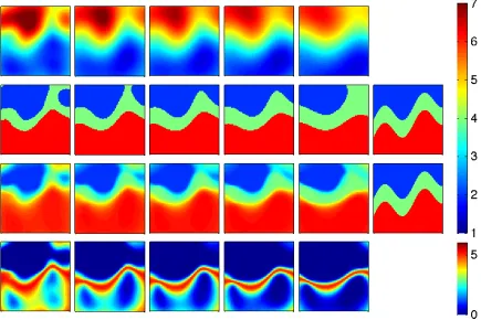
In this section we consider the inverse problem discussed in subsection3.2. We consider the Darcy model (3.4) but with a more realistic set of boundary conditions that consist of a mixed Neumman and Dirichlet conditions. For the concrete set of boundary conditions as well as the right-hand-side we use for the present example we refer the reader to [29, Section 4]. This flow model, initially used in the seminal paper of [14], has been used as a benchmark for inverse problems in [29, 22, 24]. While the mathematical analysis of subsection is3.2conducted on a model with Dirichlet boundary conditions, in order to streamline the presentation, the corresponding extension the case of mixed boundary conditions can be carried out with similar techniques.
We recall that the aim is to estimate the interface between regionsDiof different structural
geol-ogy which result in a discontinuous permeabilityκof the form (2.2). In order to generate synthetic data, we consider a trueκ†(x) = P3
i=1κiID†
i with prescribed (known) values ofκ1 = 7, κ2 = 50
andκ3 = 500. This permeability, whose plot is displayed in Figure6(top), is used in (3.4) to
gen-erate synthetic data collected from interior measurement locations (white squares in Figure6). The estimation ofκis conducted given observations of the solution of the Darcy model (3.4). To be con-crete, the observation operatorO = (O1, . . . ,O25)is defined in terms of 25 mollified Dirac deltas
{Oj}25j=1 centered at the aforementioned measurement locations and acting on the solutionpof the
Darcy flow model. For the generation of synthetic data we use a grid of160×160which, in order to avoid inverse crimes [32], is finer than the one used for the inversion (80×80). As before, ob-servations are corrupted with Gaussian noise proportional to the size of the noise-free obob-servations (Oj(p)in this case).
For the estimation of κ with the proposed Bayesian framework we assume that knowledge of three nested regions is available with the permeability values {κi}3i=1 that we use to define the
true κ†. Again, we are interested in the realistic case where the rock types of the formation are known from geologic data but the location of the interface between these rocks is uncertain. In other words, the unknowns are the geologic faciesDi that we parameterize in terms of a level set
function, i.e. Di = {x ∈ D |ci−1 ≤ u(x) < ci} with c0 = −∞, c1 = 0, c2 = 1, c3 = ∞.
Similar to the previous example, we use a prior of the form (2.9) for the level set function. In Figure
7 we display samples from the prior on the level set function (first, third and fifth rows) and the corresponding permeability mapping under the level set map (2.4)F(u)(x) = κ(x) = P3
i=1κiIDi
(second, fourth and sixth rows) for (from left to right)L = 0.2,0.3,0.35,0.4,0.5. As before, we note that the spatial correlation of the covariance function has a significant effect on the spatial correlation of the interface between the regions that define the interface between the geologic facies (alternatively, the discontinuities of κ). Longer values of L provide κ’s that seem more visually consistent with the truth. The results from Figure 8 show MCMC results from experiments with different priors corresponding to the aforementioned choices of L. The posterior mean level set functionuis displayed in the top row of Figure8. The corresponding mapping under the level set functionκ≡P3
Similar to our discussion of the preceding subsection, for the present example we are interested in the push-forward of the posteriorµy under the level set map F. More precisely,F∗µy provides
a probability description of the solution to the inverse problem of finding the permeability given observations from the Darcy flow model. In Figure8we present the mean (bottom-middle) and the variance (bottom) of F(µy) characterized by posterior samples on the level set function mapped
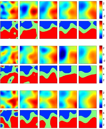
underF. In other words, these are the mean and variance from theκ’s obtained from the MCMC samples of the level / set function. As in the previous example, there is a critical value of L = 0.3 below of which the posterior estimates cannot accurately identify the main spatial features of κ†. Figure 9 shows posterior samples of the level set function (first, third and fifth rows) and the correspondingκ (second, fourth and sixth rows). The posterior samples, for values ofL above the critical valueL= 0.3, capture the main spatial features from the truth. There is, however, substantial uncertainty in the location of the interfaces. Our results offer evidence that this uncertainty can be properly captured with our level set Bayesian framework. Statistical measures of F∗µy (i.e.
the posterior permeability measure on κ) is essential in practice. The proper quantification of the uncertainty in the unknown geologic facies is vital for the proper assessment of the environmental impact in applications such as CO2 capture and storage, nuclear waste disposal and enhanced oil
recovery.
In Figure 6 (bottom-right) we show the ACF of the first KL mode of level set function from different MCMC chains corresponding to different priors defined by the choices ofLindicated pre-viously. In contrast to the previous example, here we cannot appreciate substantial differences in the efficiency of the chain with respect to the selected values ofL. However, we note that ACF exhibits a slow decay and thus long chains and/or multiple chains are need to properly explore the poste-rior. For the choice of L = 0.4 we consider50 multiple MCMC chains. Our MCMC chains pass the Gelman-Rubin test [10] as we can note from Figure 6(bottom-left) where we show the PSRF computed from MCMC samples of the level set functionu (red-solid line) and the corresponding mapping, under the level set map, into the permeabilitiesκ(blue-dotted line). As indicated earlier, we may potentially increase the number of multiple chains and thus the number of uncorrelated samples form the posterior.
Finally, in Figure10we show the prior and posterior densities of the first DCT coefficients on the κobtained from the MCMC samples of the level set function (the vertical dotted line corresponds to the DCT coefficient of the truthκ†). For some of these modes we clearly see that the posterior is concentrated around the truth. However, for the modeξ4,4 we note that the posterior is quite close
to the prior indicating that the data have not informed this mode in any significant way.
4.5
Structural Geology: Layer Model
0 1 2 3 4 5 6 0 1 2 3 4 5 6 x y 1 2 3 4 5 6 7
0 1 2 3 4 5 6 7 8 9 10
1 1.05 1.1 1.15 1.2
MCMC steps (x105)
PSRF
κ
level−set
[image:23.612.149.444.93.352.2]0 1000 2000 3000 4000 5000 6000 0 0.1 0.2 0.3 0.4 0.5 0.6 0.7 0.8 0.9 1 lag ACF L=0.2 L=0.3 L=0.35 L=0.4 L=0.5
Figure 6: Identification of structural geology (channel model). Top: Trueκin eq. (3.4). Bottom-left: PSRF from multiple chains withL= 0.4in (2.8). Bottom-right: ACF of first KL mode of the level set function from single-chain MCMC with different choices ofL.
data is conducted as described in the preceding subsection. For this example we consider the Gaus-sian prior on the level set defined by (2.8). Since for this case the operatorC is diagonalisable by cosine functions, we use the fast Fourier transform to sample from the corresponding Gaussian measureN(0,C)required by the pCN-MCMC algorithm.
The tunable parameterα in the covariance operator (2.8) determines the regularity of the cor-responding samples of the Gaussian prior (see for example [45]). Indeed, in Figure 12 we show samples from the prior on the level set function (first, third and fifth rows) and the correspondingκ (second, fourth and sixth rows) for (from left to right)α= 1.5,2.0,2.5,3.0,3.5. Indeed, changes in αhave a dramatic effect on the regularity of the interface between the different regions. We therefore expect strong effect on the resulting posterior on the level set and thus on the permeability.
In Figure13we display numerical results from MCMC chains with different priors correspond-ing to (from left to right)α= 1.5,2.0,2.5,3.0,3.5. In Figure13we present the MCMC mean of the level set function.The correspondingκ is shown in the top-middle of Figure13. In this figure we additionally display the mean (bottom-middle) and the variance (bottom) of theκ’s obtained from the MCMC samples of the level set function. Above a critical valueα= 2.5we obtain a reasonable identification of the layer permeability with a small uncertainty (quantified by the variance). Figure
−20 0 2 4 6 1 2 3 4 ξ1,1
posterior density of
ξ1,1
prior posterior
−20 −1 0 1 2
2 4 6 8
ξ2,2
posterior density of
ξ2,2
prior posterior
−10 −0.5 0 0.5 1
2 4 6
ξ4,2
posterior density of
ξ4,2
prior posterior
−20 −1 0 1 2
2 4 6
ξ1,3
posterior density of
ξ1,3
prior posterior
−10 −0.5 0 0.5 1
2 4 6
ξ2,4
posterior density of
ξ2,4
prior posterior
−100000 −5000 0 5000
2 4 6
ξ4,4
posterior density of
[image:27.612.103.488.100.308.2]ξ4,4 prior posterior
Figure 10: Identification of structural geology (channel model). Densities of the prior and posterior of some DCT coefficients of theκ’s obtained from MCMC samples on the level set for L = 0.4
(vertical dotted line indicates the truth).
Figure11(bottom-right) shows the ACF of the first KL mode of level set function from MCMC experiments with different priors withα’s as before. The efficiency of the MCMC chain does not seem to vary significantly for the values above the critical value ofα. However, as in the previous examples a slow decay in the ACF is obtained. An experiment using 50multiple MCMC chains initialized randomly from the prior reveals that the Gelman-Rubin diagnostic test [10] is passed for α = 2.5as we can observe from Figure11(bottom-left) where we the display PSRF from MCMC samples of the level set function (red-solid line) and the corresponding mapping into theκ (blue-dotted line). In Figure15we show the prior and posterior densities of the DCT coefficients on theκ obtained from the MCMC samples of the level set function (the vertical dotted line corresponds to the truth DCT coefficient). We see clearly that the DCT coefficients are substantially informed by the data although the spread around the truth confirms the variability in the location of the interface between the layers that we can ascertain from the posterior samples (see Figure14).
5
Conclusions
The primary contributions of this paper are:
• We have formulated geometric inverse problems within the Bayesian framework.
0 1 2 3 4 5 6 0 1 2 3 4 5 6 x y 1 2 3 4 5 6 7
0 1 2 3 4 5 6 7 8 9 10
1 1.1 1.2 1.3 1.4 1.5 1.6 1.7 1.8
MCMC steps (x105)
PSRF
κ
level−set
0 1000 2000 3000 4000 5000 6000 7000 8000 9000 10000
[image:28.612.147.441.95.351.2]0 0.1 0.2 0.3 0.4 0.5 0.6 0.7 0.8 0.9 1 lag ACF α=1.5 α=2.0 α=2.5 α=3.0 α=3.5
Figure 11: Identification of structural geology (layer model). Top: Trueκin eq. (3.4). Bottom-left: PSRF from multiple chains withα = 2.5in (2.9). Bottom-right: ACF of first KL mode of the level set function from single-chain single-chain MCMC with different choices ofα.
• The framework also leads to the use of state-of-the-art function-space MCMC methods for sampling of the posterior distribution on the level set function. An explicit motion law for the interfaces is not needed: the MCMC accept-reject mechanism implicitly moves them.
• We have studied two examples: inverse source reconstruction and an inverse conductivity problem. In both cases we have demonstrated that, with appropriate choice of priors, the abstract theory applies. We have also highlighted the behavior of the algorithms when applied to these problems.
1 2 3 4 0 0.2 0.4 0.6 0.8 1 ξ1,1
posterior density of
ξ1,1
prior posterior
−20 −1 0 1 2
2 4 6
ξ2,2
posterior density of
ξ2,2
prior posterior
−10 −0.5 0 0.5 1
2 4 6 8
ξ4,2
posterior density of
ξ4,2
prior posterior
−20 −1 0 1 2
2 4 6
ξ1,3
posterior density of
ξ1,3
prior posterior
−10 −0.5 0 0.5 1
0.2 0.4 0.6 0.8 1 ξ2,4
posterior density of
ξ2,4
prior posterior
−50000 0 5000
0.2 0.4 0.6 0.8 1 ξ4,4
posterior density of
ξ4,4
[image:32.612.100.490.100.307.2]prior posterior
Figure 15: Identification of structural geology (layer model). Densities of the prior and posterior of some DCT coefficients of theκ’s obtained from MCMC samples on the level set for L = 0.4
(vertical dotted line indicates the truth).
so in a way that avoids creating flat level set functions underlying the permeability. Indeed, we note that the posterior samples of the level set function inherit the same properties from the ones of the prior. Therefore, the probability of obtaining a level set function which takes any given value on a set of positive measure is zero under the posterior, as it is under the prior. This fact promotes very desirable, and automatic, algorithmic robustness.
Natural directions for future research include the following:
• The numerical results for the two examples that we consider demonstrate the sensitive de-pendence of the posterior distribution on the length-scale parameter of our Gaussian priors. It would be natural to study automatic selection techniques for this parameter, including hierar-chical Bayesian modelling.
• We have assumed that the values of κi on each unknown domain Di are both known and
constant. It would be interesting, and possible, to relax either or both of these assumptions, as was done in the finite geometric parameterizations considered in [27].
• The numerical results also indicate that initialization of the MCMC method for the level set function can have significant impact on the performance of the inversion technique; it would be interesting to study this issue more systematically.
is assumed for the regions{Di}ni=1 see Figure 16(a). However, we comment that there exist
objects with non-nested regions, such as the one depicted in Figure16(b), which can not be represented by a single level set function. . It would be of interest to extend this work to the consideration of vector-valued level set functions. In the case of binary obstacles, it is enough to represent the shape via a single level set function (cf. [43]). However, in the case ofn-ary obstacles or even more complex geometric objects, the representation is more complicated; see the review papers [18,19,46] for more details.
[image:33.612.155.439.229.381.2](a) Nested regions (b) Non-nested regions
Figure 16: Nested regions and non-nested regions
• The Bayesian framework could be potentially combined with other parameterizations of un-kwon geometries. For example, the pluri Gaussian approach has been used with EnKF in [35] to identify geologic facies.
AcknowledgmentsYL is is supported by EPSRC as part of the MASDOC DTC at the University of
Warwick with grant No. EP/HO23364/1. AMS is supported by the (UK) EPSRC Programme Grant EQUIP, and by the (US) Ofice of Naval Research.
References
[1] R. J. Adler and J. E. Taylor. Random Fields and Geometry, volume 115 of Springer Mono-graphs in Mathematics. Springer, 2007.
[2] G. Alessandrini. On the identification of the leading coefficient of an elliptic equation. Boll. Un. Mat. Ital. C (6), 4(1):87–111, 1985.
[4] T. Arbogast, M. F. Wheeler, and I. Yotov. Mixed finite elements for elliptic problems with tensor coefficients as cell-centered finite differences.SIAM J. Numer. Anal., 34:828–852, 1997.
[5] M. Armstrong, A. Galli, H. Beucher, G. Le Loc’h, D. Renard, B. Doligez, R. Eschard, and F. Geffroy. Plurigaussian Simulations in Geosciences. 2nd revised edition edition, 2011.
[6] A. Astrakova and D.S. Oliver. Conditioning truncated pluri-Gaussian models to facies obser-vations in ensemble-Kalman-based data assimilation. Mathematical Geosciences, page Pub-lished online April 2014, 2014.
[7] V. I. Bogachev. Gaussian Measures, volume 62 of Mathematical Surveys and Monographs. American Mathematical Society, 1998.
[8] A. Bonito, R. A. DeVore, and R. H. Nochetto. Adaptive finite element methods for elliptic problems with discontinuous coefficients. SIAM Journal on Numerical Analysis, 51(6):3106– 3134, 2013.
[9] L. Borcea. Electrical impedance tomography. Inverse Problems, 18(6):R99, 2002.
[10] S.P. Brooks and A. Gelman. General methods for monitoring convergence of iterative simula-tions. Journal of Computational and Graphical Statistics, 7:434–455, December 1998.
[11] M. Burger. A level set method for inverse problems. Inverse Problems, 17(5):1327, 2001.
[12] M. Burger. A framework for the construction of level set methods for shape optimization and reconstruction. Interfaces and Free Boundaries, 5:301–329, 2003.
[13] M. Burger and S. Osher. A survey on level set methods for inverse problems and optimal design. Europ. J. Appl. Math., 16:263–301, 2005.
[14] J. Carrera and S. P. Neuman. Estimation of aquifer parameters under transient and steady state conditions: 3. application to synthetic and field data. Water Resources Research, 22.
[15] E. T. Chung, T. F. Chan, and X. C. Tai. Electrical impedance tomography using level set representation and total variational regularization. J. Comp. Phys., 205:357–372, 2005.
[16] S. L. Cotter, G. O. Roberts, A. M. Stuart, and D. White. MCMC methods for functions: modifying old algorithms to make them faster. Statistical Science, 28(3):424–446, 2013.
[17] M. Dashti and A. M. Stuart. The Bayesian approach to inverse problems. In Handbook of Uncertainty Quantification, page arxiv.1302.6989. Springer, 2016.
[19] O. Dorn and D. Lesselier. Level set methods for inverse scattering–some recent developments.
Inverse Problems, 25(12):125001, 2009.
[20] H. W. Engl, M. Hanke, and A. Neubauer. Regularization of Inverse Problems, volume 375. Springer, 1996.
[21] L.C. Evansand and J. Spruck. Motion of level sets by mean curvature I.J. Diff. Geom, 33:635– 681, 1991.
[22] M. Hanke. A regularizing Levenberg-Marquardt scheme, with applications to inverse ground-water filtration problems. Inverse Problems, 13:79–95, 1997.
[23] F. Hettlich and W. Rundell. Iterative methods for the reconstruction of an inverse potential problem. Inverse Problems, 12(3):251, 1996.
[24] M. A. Iglesias and C. Dawson. An iterative representer-based scheme for data inversion in reservoir modeling. Inverse Problems, 25:035006, 2009.
[25] M. A. Iglesias, K. Law, and A. M. Stuart. Ensemble Kalman methods for inverse problems.
Inverse Problems, 29(4):045001, 2013.
[26] M. A. Iglesias, K. J. H. Law, and A. M. Stuart. Evaluation of Gaussian approximations for data assimilation in reservoir models. Computational Geosciences, 17:851–885, 2013.
[27] M. A. Iglesias, K. Lin, and A. M. Stuart. Well-posed Bayesian geometric inverse problems arising in subsurface flow. arXiv:1401.5571v2, 2014.
[28] M. A. Iglesias and D. McLaughlin. Level-set techniques for facies identification in reservoir modeling. Inverse Problems, 27(3):035008, 2011.
[29] M.A. Iglesias, K.J.H. Law, and A.M. Stuart. Ensemble Kalman methods for inverse problems.
Inverse Problems, 29(4):045001, 2013.
[30] V. Isakov. Inverse Source Problems, volume 34 of Mathematical Surveys and Monographs. American Mathematical Society, 1990.
[31] V. Isakov. Inverse Problems for Partial Differential Equations. Applied Mathematical Sci-ences. Springer, 2rd edition, 2006.
[32] J. P. Kaipio and E. Somersalo. Statistical and Computational Inverse Problems, volume 160. Springer, 2005.
[34] J. Lie, M. Lysaker, and X. C. Tai. A variant of the level set method and applications to image segmentation. Math. Comput., 75:1155–1174, 2006.
[35] Ning Liu and Dean S Oliver. Ensemble kalman filter for automatic history matching of geo-logic facies. Journal of Petroleum Science and Engineering, 47(3):147–161, 2005.
[36] R.J. Lorentzen, K.M. Flornes, and G. Nævdal. History matching channelized reservoirs using the ensemble Kalman filter.
[37] R.J. Lorentzen, G. Nævdal, and A. Shafieirad. Estimating facies fields by use of the ensemble kalman filter and distance functions–applied to shallow-marine environments.
[38] B. Merriman, R. Caflisch, and S. Osher. Level set methods, with an application to modeling the growth of thin films. In Free Boundary Value Problems, Theory and Applications, pages 51–70. CRC Press, 1998.
[39] S. D. Oliver, C. A. Reynolds, and N. Liu. Inverse Theory for Petroleum Reservoir Character-ization and History Matching. Cambridge University Press, 2008.
[40] Jing Ping and Dongxiao Zhang. History matching of channelized reservoirs with vector-based level-set parameterization.
[41] G. R. Richter. An inverse problem for the steady state diffusion equation. SIAM Journal on Applied Mathematics, 41(2):210–221, 1981.
[42] T. Ilmanen S. Angenent and D. L. Chopp. A computed example of nonuniqueness of mean curvature flow inR3. Communications in Partial Differential Equations, 20:1937–1958, 1995.
[43] F. Santosa. A level-set approach for inverse problems involving obstacles. ESAIM: Control, Optimisation and Calculus of Variations, 1:17–33, 1996.
[44] E. M. Stein and R. Shakarchi. Real Analysis : Measure Theory, Integration, and Hilbert Spaces. Princeton University Press, 2009.
[45] A. M. Stuart. Inverse problems: A Bayesian perspective.Acta Numerica, 19:451–559, 5 2010.
[46] X. C. Tai and T. F. Chan. A survey on multiple level set methods with applications for identify-ing piecewise constant functions. International Journal of Numerical Analysis and Modeling, 1:25–47, 2004.
[47] L. A. Vese and T. F. Chan. A multiphase level set framework for image segmentation using the mumford-shah model. Int. J. Comput. Vis., 50:271–293, 2002.
[49] J. Xie, Y. Efendiev, A. Datta-Gupta, et al. Uncertainty quantification in history matching of channelized reservoirs using markov chain level set approaches. InSPE Reservoir Simulation Symposium. Society of Petroleum Engineers, 2011.
6
Appendix 1
Proof of Theorem2.2. Notice that the random variabley|u is distributed according to the measure
Qu, which is the translate ofQ0byG(u), satisfyingQu Q0 with Radon-Nikodym derivative
dQu
dQ0(y)∝exp
−Φ(u;y);
where Φ : U × RJ →
R is the least squares function given in (2.6). Thus for the given data y,
Φ(u;y)is up to a constant, thenegative log likelihood. We denote byν0 the product measure
ν0(du, dy) = µ0(du)Q0(dy). (6.1)
Suppose that Φ(·,·) is ν0 measurable, then the random variable (u, y) ∈ U × Y is distributed
according toν(du, dy)with
dν dν0
(u, y)∝exp−Φ(u;y).
From Assumptions2.1(ii) and the continuity ofΦ(u;y)with respect toy, we know thatΦ(·;·) :
U ×Y → Ris continuous ν0−almost surely. Then it follows from Lemma6.1 below that Φ(·;·)
isν0-measurable. On the other hand, by Assumptions2.1(i), for|y|Γ ≤ r, we obtain the upper and
lower bound forZ,
0<exp(−K(r, κmin))≤Z =
Z
U
exp(−Φ(u;y))µ0(du)≤1
Thus the measure is normalizable and applying the Bayes’ Theorem 3.4 from [17] yields the exis-tence ofµy.
LetZ =Z(y)andZ0 =Z(y0)be the normalization constants forµy andµy0, i.e.
Z =
Z
U
exp(−Φ(u;y))µ0(du), Z0 =
Z
U
exp(−Φ(u;y0))µ0(du)
We have seen above that
1≥Z, Z0 ≥exp(−K(r, κmin))>0.
From Assumptions2.1(iii),
|Z−Z0| ≤
Z
|exp(−Φ(u;y))−exp(−Φ(u;y0))|µ0(du)≤
Z
|Φ(u;y)−Φ(u;y0)|µ0(du)≤C(r)|y−y0|Γ
Thus, by the definition of Hellinger distance, we have
2dHell(µy, µy
0
)2 =
Z
Z−1/2exp
−1
2Φ(u;y)
−(Z0)−1/2exp
−1
2Φ(u;y
0)
2
where
I1 =
2 Z Z exp −1
2Φ(u;y)
−exp
−1
2Φ(u;y
0
)
2
µ0(du)
I2 = 2|Z−1/2−(Z0)−1/2|2
Z
exp(−Φ(u;y0))µ0(du)
Applying (i) and (iii) in Assumptions2.1again yields
Z
2I1 ≤C(r)|y−y
0|2 Γ
and
I2 ≤C(r)|Z−1/2−(Z0)−1/2|2 ≤C(r)(Z−3∨(Z0)−3)|Z−Z0|2 ≤C(r)|y−y0|2Γ
Therefore the proof that the measure is Lipschitz is completed by combining the preceding esti-mates. The final statement follows as in [45], after noting that f ∈ L2µ0(U;S) implies that f ∈
L2
µy(U;S), sinceΦ(·;y)≥0.
Lemma 6.1. LetU be a separable Banach space and(U,Σ, µ)be a complete probability space with
σ-algebra Σ. If a functional F : U → R is continuousµ-almost surely, i.e.µ(M) = 1 whereM denotes the set of the continuity points ofF, thenF isΣ-measurable.
Proof. By the definition of measurability, it suffices to show that for anyc > 0
S :={u∈U | F(u)> c} ∈Σ.
One can writeSasS = (S∩M)∪(S\M). SinceF is continuousµ-almost surely,Mis measurable
andµ(M) = 1. It follows from the completeness of the measureµthatS \M is measurable and
µ(S\M) = 0. Now we claim thatS∩M is also measurable. DenoteBδ(u)⊂ U to be the ball of
radiusδ centered atu ∈U. For eachv ∈ S∩M, asF is continuous atv, there existsδv >0such
that ifv0 ∈Bδv(v), thenF(v 0)> c
. ThereforeS∩M can be written as
S∩M =M\ [
v∈S∩M
Bδv(v)
that is the intersection of the measurable setM with the open set S
v∈S∩M Bδv(v). So S ∩M is
measurable. Then it follows thatF isΣ-measurable.
Proof of Proposition2.4. “⇐=.” Let {uε} denote any approximating family of level set functions
with limituasε→0inC(D;R) :kuε−ukC(D)< ε→0. LetDi,ε, D0i,εbe the sets defined in (2.3)
associated with the approximating level set functionuεand defineκ=F(u)by (2.4) and, similarly,
κε:=F(uε). Letm(A)denote the Lebesgue measure of the setA.
Suppose thatm(D0
i) = 0, i= 1,· · · , n−1. Let{uε}be the above approximating functions. We
shall provekκε−κkLq(D) →0. In fact, we can write
κε(x)−κ(x) =Pni=1Pjn=1(κi−κj)IDi,ε∩Dj(x)
=Pn
By the definition ofuε, for anyx∈D
u(x)−ε < uε(x)< u(x) +ε (6.2)
Thus for|j −i| > 1 andεsufficiently small, Di,ε∩Dj = ∅. For the case that|i−j| = 1, from
(6.2), it is easy to verify that
Di,ε∩Di+1 ⊂Dei,ε := {x∈D|ci ≤u(x)< ci+ε} →D0i, i = 1,· · · , n−1 (6.3) Di,ε∩Di−1 ⊂Dbi−1,ε := {x∈D|ci−1−ε < u(x)< ci−1} →∅, i= 2,· · ·n (6.4)
asε→0. By this and the assumption thatm(D0
i) = 0, we have thatm(Di,ε∩Dj)→0ifi6=j.
Furthermore, the Lebesgue’s dominated convergence theorem yields
kκε−κkqLq(D)=
n
X
i,j=1,i6=j
Z
Di,ε∩Dj
|κi−κj|qdx→0
asε→0. Therefore,F is continuous atu.
“=⇒.” We prove this by contradiction. Suppose that there existsi∗ such thatm(D0
i∗) 6= 0. We
defineuε :=u−ε, then it is clear thatkuε−ukC(D) →0asε→0. By the same argument used in
proving the sufficiency,
kκε−κkqLq(D)=
n−1
X
i=1
Z
e
Di,ε∪Dbi,ε
|κi+1−κi|qdx→
n−1 X i=1 Z D0 i
|κi+1−κi|qdx >
Z
D0
i∗
|κi∗+1−κi∗|qdx >0
where we have usedm(D0
i∗) 6= 0in the last inequality. However, this contradicts with the
assump-tion thatF is continuous atu.
7
Appendix 2
Recall the Gaussian measureµ0 =N(0,C)on the function spaceHwhereC =Ci,H=Hi, i= 1,2
given in subsection2.5. These measures can be constructed as Gaussian random fields.
Let(Ω,F,P)be a complete probability space, i.e. if A ∈ F with P(A) = 0, thenP(B) = 0
for B ⊂ A. A random field on D is a measurable mapping u : D × Ω → R. Thus, for any x ∈ D,u(x;·)is a random variable inR; whilst for any ω ∈ Ω,u(·;ω) :D → Ris a vector field. Denote by(RN,B(
RN),P)the probability space of i.i.d standard Gaussian sequences equipped with
product σ-algebra and product measure. In this paper, we consider (Ω,F,P) as the completion of (RN,B(RN),P) in which case the σ-algebra F consists of all sets of the type A∪ B, where
A∈ B(RN)andB ⊂N ∈ B(
RN)withP(N) = 0. Letω ={ξk}∞k=1 ∈Ω =RNbe an i.i.d sequence
with ξ1 ∼ N(0,1), and consider the random function u ∈ H defined via the Karhunen-Lo´eve