Abstract— Face Biometrics is a science of automatically identifying individuals based on their unique facial features. The paper presents neural network classifier(Radial Basis Function Network) to detect frontal views of faces. The curvelet transform, Linear Discriminant Analysis(LDA) are used to extract features from facial images first, and Radial Basis Function Network(RBFN) is used to classify the facial images based on features. Radial Basis Function Network is used to reduce the number of misclassification caused by not-linearly separable classes. 200 images are taken from ORL database and was tested, where the parameters like recognition rate, acceptance ratio and execution time performance are calculated. Neural network based face recognition is robust and has better performance of recognition rate 98.6% and acceptance ratio 85 %.
Index Terms - Face recognition, Curvelet Transform, Linear Discriminant analysis , Radial Basis Function Network ,Recognition rate, Acceptance ratio, Execution time.
I. INTRODUCTION
Face recognition [1] has become one of the interesting and most challenging task in the pattern recognition field. The problem of face recognition is very challenging for the appearance caused by change in illumination, facial features, occlusions, etc. Face recognition is implemented into image organizing software,web applications,mobile devices and passports already contain face biometric data.The paper presents a RBF classifier and LDA based algorithm gives efficient and robust face recognition. In general, there are three important methods for face recognition [1] such as Holistic method, feature-based method and hybrid method. The holistic method is used in which the input is taken as the whole face region and based on LDA it simplifies a featureset into lower dimension while retaining the characteristics of featureset.
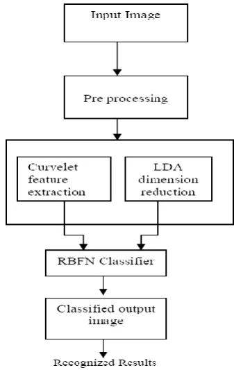
The technique is separated into three main steps namely; preprocessing, feature extraction, classification and recognition as shown in figure1.Different feature extraction methods of face recognition and RBF classifier are discussed.The paper is organized as follows:
Manuscript received July 06, 2011; revised August 12, 2011.
V. Radha is with the Department of Computer Science, Avinashilingam Institute for Home Science and Higher Education for Women University, Coimbatore, Tamilnadu, PIN 641043 India. (phone: +91422-2404983; e-mail:[email protected]).
N. Nallammal is the Research Scholar with the Department of Computer Science, Avinashilingam Institute for Home Science & Higher
Education for
WomenUniversity,Coimbatore-641043,Tamilnadu,India.(Mobile
:9698192480,e-mail::[email protected]).
Section 2 presence the overview of Pre-processing , Section 3 gives brief review of feature extraction using curvelets and LDA algorithm, Section 4 Presence Classification ,Section 5 Deals with Analysis based on result , Conclusion is discussed in Section 6
Fig 1 Block Diagram of Face Recognition System
II. OVERVIEWOFPRE-PROCESSINGTECHNIQUE Pre-processing is carried out for the following two purposes
(i) To reduce noise and possible convolute effects of interfering system‟
[image:1.595.328.497.279.546.2](ii) To transform the image into a different space where classification may prove easier by exploitation of certain features.
Fig 2 Pre-processing Block Diagram
Neural Network Based Face Recognition Using
RBFN Classifier
A. Histogram Equalization
Pre-processing Block Diagram shows (Figure 2.) the mean centering, raw images cropped, size reduced , histogram equalized and then adaptively mean centered and changes to vectors.
III. Brief Review of Feature Extraction Using Curvelets And LDA Algorithm
Feature extraction for face representation is one of the main issue of face recognition system. Among various solutions to the problem, the most successful seems to be those appearance-based approaches, which generally operate directly on images or appearances of face objects and process the image as two-dimensional patterns. Feature extraction means it represents the data in a lower dimensional space computed through a linear or non-linear transformation satisfying certain properties. Statistical techniques have been widely used for face recognition and facial analysis to extract the abstract features of the face patterns. Curvelets and LDA [8] are two main techniques used for data reduction and feature extraction in the appearance-based approaches.
Feature extraction is a key step prior to face recognition. Extraction of a representative feature set can greatly enhance the performance of any face recognition system. Direct use of pixel values as features is not possible due to huge dimensionality of the images. To reduce the dimensionality, LDA is employed to obtain a lower dimensional representation of the data in standard eigenface[7]. Nowadays, multiresolution analysis is often performed as a preprocessing step to dimensionality reduction.
A. Curvelet Based Feature Extraction
Curvelet transform used to extract features from facial images, and then uses RBFN to classify facial images based on features. curvelet transform has been developed especially to represent objects with ‘curve-punctuated
smoothness’ [9] i.e. objects which display smoothness except for discontinuity along a general curve; images with edges are good examples of this kind of objects. In a two dimensional image two adjacent regions can often have differing pixel values. Such a gray scale image will have a lot of “edges” i.e. discontinuity along a general curve and consequently curvelet transform will capture this edge information. To form an efficient feature set it is crucial to collect these interesting edge information which in turn increases the discriminatory power of a recognition system[9]. The face recognition system is divided into two stages: training stage and classification stage. In training stage, the images are decomposed into its approximate and detailed components using curvelet transform. These sub-images thus obtained are called curvefaces. These
curvefaces greatly reduces the dimensionality of the original image. Then LDA is applied on selected subbands, which further reduces the dimension of image data. Thereafter only the approximate components are selected to perform further
computations for maximum variance to represent an efficient feature set is produced. In classification stage, test images are subjected to the same operations and are transformed to the same LDA representational basis. Figure 3 shows the curvelet coefficients of a face from ORL dataset decomposed at scale = 2 and angle = 8.
Curvelet transform is multiscale and multidirectional. Curvelets exhibit highly anisotropic shape obeying parabolic-scaling relationship.Like wavelet and ridgelet transform, the second continuous curvelet transform is also fallen into the category of sparseness theory. It can be used to represent sparsely signal or function by applying the inner product of basis function and signal or function.
A polar „wedge‟ represented by shadow region of Figure. 3,it shows the division of wedges of the fourier frequency plane. The wedges are the result of partitioning the fourier plane in radial (concentric circles) and angular divisions. Concentric circles are responsible for decomposition of the image in multiple scales (used for bandpassing the image) and angular divisions corresponding to different angles or orientation. So, to address a particular wedge one needs to define the scale and angle first.
(1)Uniform rotation angle serial
Fig 3 Curvelet representation in the frequency domain
(1)
(2) Shift parameter
(2) The above concept, the curvelet can be defined as a function of x =(x1, x2) at scale 2-j, orientation θl, and position xk(j,l) by equation (3),
(3)
where Rθ =Rotation in radius
Then the continuous curvelet transform can be defined by equation (4)
Based on Plancherel Therory, the following formula can be deduced from the equation (5),
(5) Set the input f[t1,t2] (0≤t1, t2<n) in the spatial Cartesian, then the discrete form of above continuous curvelet transform can be expressed as the following equation (6)
(6) The discrete curvelet transform can be implemented by a „wrapping‟ algorithm. In this algorithm, four steps are carried out:
(1) Application of 2D fast fourier transform to the image. (2) Formation of a product of Uj for each scale and angle. (3) Wrapping of this product around the origin.
(4) Application of a 2D inverse fast Fourier transform, resulting in discrete curvelet coefficients.
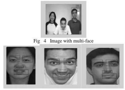
[image:3.595.65.269.339.485.2]Fig 4 Image with multi-face
Fig 5 Extracted facial features
B. Linear Discriminant Analysis
LDA is a common statistical technique to findout the patterns in high dimensional data [8].Feature extraction, also called dimensionality reduction is done by LDA for three main reasons they are
i) To reduce dimension of the data to more tractable limits
ii) To capture salient class-specific features of the data,
iii) To eliminate redundancy.
Once the face is normalized and feature extraction is performed as shown in figure 5 .The information provided is useful for distinguishing faces of different persons and stable with respect to the geometrical and photometrical variations.
LDA searches the directions for maximum discrimination of classes in addition to dimensionality reduction. To achieve this goal, within-class and between-class matrices are defined. A within-between-class [8] scatter matrix is the scatter of the samples around their respective class means mi
(7) where Σi denotes the covariance matrix of i-th class. The between-class scatter matrix is the scatter of class means mi around the mixture mean m is given by equation (8)
(8) Finally, the mixture scatter matrix is the covariance of all sample class assignments defined by equation (9)
(9) Different objective functions have been used as LDA criteria mainly based on a family of function of scatter matrices. For example, the maximization of the following objective functions have been proposed by equation (10)
(10) In LDA, the optimum linear transform is composed of p(≤ n) eigenvectors of Σ w-1 Σ b corresponding to its p largest eigenvalues. Alternatively, Σ w-1 Σ b can be used for LDA, simple analysis shows that both Σ w-1 Σ b and Σ w-1 Σ have the same eigenvector matrices. In general, Σb is not full rank and therefore not a covariance matrix, hence Σca used in place of Σb . The computation of the eigenvector matrix ΦLDAof Σw-1 Σ is equivalent to the solution of the generalized eigenvalue problem ΣΦLDA =Σw ΦLDA Λ where Λ is the generalized eigenvalue matrix. The assumption of positive definite matrix Σw , there exists a symmetric Σw
-1/2
such that the problem can be reduced to a symmetric eigenvalue problem denotes the equation(11)
(11) Outputs of dimension reduction part are 100×1 vectors which are used to construct within class scatter matrix and covariance matrix. The significant eigenvectors of Σ-1w Σ can be used for separability of classes in addition to dimension reduction. Using 100×1 vectors, Σ-1 w Σ computed and then eigenvectors related to the greater eigenvalues are selected. To consider 10 classes and 9 major eigenvectors associated with non-zero eigenvalues which have separability capability. It is clear that extracting all 9 LDA features increase the discriminatory power of the method. This produces 9×1 vectors which are used as input of RBFN, first covariance and within class scatter matrices are estimated and then significant eigenvector of
Σ-1
IV. CLASSIFIERDESIGN
Neural networks have been employed and compared to conventional classifiers for a number of classification problems. The results shows that the accuracy of the neural network approaches equivalent to, or slightly better than, other methods. It is due to the simplicity, generality and good learning ability of the neural networks[4]. RBFN have found to be very attractive for many engineering problem because: (1) they are universal approximators, (2) they have a very compact topology and (3) their learning speed is very fast because of their locally tuned neurons. Therefore the RBF neural networks serve as an excellent role for pattern applications carried out to make the learning process, this type of classification is faster than the other network models.
The RBF classifier is a hidden layer neural network with several forms of radial basis activation functions. The most common one is the Gaussian function defined by equation (12)
(12)
In a RBF network, a neuron of the hidden layer is activated whenever the input vector is close enough to its center vector mj. There are several techniques and heuristics
for optimizing the basis functions parameters and determining the number of hidden neurons needed to best classification[4]. This work implements the Gaussian Mixture Model algorithm to train the network. The basis functions are the components of a mixture density model. The number of hidden neurons are equal to the number of basis functions are treated as an input to the model and is typically much less than the total number of input data points {xi}. The second layer of the RBF network, which is the output layer, comprises one neuron to each individual. Their output are linear functions of the outputs of the neurons in the hidden layer and is equivalent to an OR operator. The final classification is given by the output neuron with the greatest output. With RBF networks, the regions of the input space associated to each individual can present an arbitrary form. Also, disjoint regions can be associated to the same individual to render, for example, very different angles of vision or different facial expressions.
A. RBF Network Structure
RBFN contains one input layer and one output layer with a single hidden layer as shown in figure 6. The radial basis functions are used within the hidden layer. The training is done by adjusting the center parameters in the radial basis functions that will be used to calculate the connection strengths between the hidden layer and output layer[4]
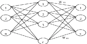
[image:4.595.71.246.683.773.2]Input Layer RBF Units Output Layer Fig 6 RBF neural network structure
An RBF neural network structure is similar to a traditional three-layer feed forward neural network. The construction of the RBF neural network involves three different layers with feed forward architecture. The input layer of this network is a set of n units, which accept the elements of an n -dimensional input feature vector. The input units are fully connected to the hidden layer with r hidden units. Connections between the input and hidden layers have unit weights and, as a result, do not have to be trained. The goal of the hidden layer is to cluster the data and reduce its dimensionality. In this structure hidden layer is named RBF units. The RBF units are also fully connected to the output layer. The output layer supplies the response of neural network to the activation pattern applied to the input layer. The transformation from the input space to the RBF-unit space is nonlinear, whereas the transformation from the RBF unit space to the output space is linear[6].
The RBF neural network is a class of neural networks, where the activation function of the hidden units is determined by the distance between the input vector and a prototype vector. The activation function of the RBF units is expressed as equation (13)
(13) Where x is an n-dimensional input feature vector, ci is an n
-dimensional vector called the center of the RBF unit , σi is
the width of RBF unit and r is the number of the RBF units. Typically the activation function of the RBF units is chosen as a Gaussian function with mean vector ci and variance
vector Ri (x) shows as equation (14)
(14)
σi2 - Represents the diagonal entries of covariance matrix of Gaussian function.
The output units are linear and therefore the response of the J th output unit for input x is given as equation (15)
(15)
where W2 (i, j) Connection weight of the i-th RBF unit to the
j-th output node ,b( j) is the bias of the jth output. The bias is omitted in this network in order to reduce network complexity shows equation (16).
RBF neural network classifier can be viewed as a function mapping interplant that tries to construct hyper surfaces, one for each class, by taking a linear combination of the RBF units. These hyper surfaces can be viewed as discriminant functions, where the surface has a high value for the class it represents and a low value for all others. An unknown input feature vector is classified as belonging to class associated with the hyper surface with the largest output at that point. In this case the RBF units‟ serve as components in a finite expansion of the desired hyper surface where the component coefficients (the weights) have to be trained for designing a classifier based on RBF neural network and set the number of input nodes in the input layer of neural network equal to the number of feature vector elements. The number of nodes in the output layer is set to the number of image classes.
V. ANALYSIS OF THE RESULT
[image:5.595.325.528.48.184.2]In this paper features are extracted first and dimension reduction is carried out from facial images .RBFN is used to classify the facial images . Table 1 shows that out of 200 images have been used most of them recognized by RBFN and the best average recognition rate is 98.6% .The performance of recognition rate is better than the other techniques.
Fig 7 No.of.Images Vs Acceptance Ratio
Table 1
Fig 8 No.of.Images Vs Execution time(Seconds)
[image:5.595.323.527.298.422.2]Table1 shows the acceptance ratio of LDA is 83.5% compared with curvelets acceptance ratio is high that is 84.9%.The proposed method acceptance ratio is 87.1% represents the figure 7 it is better than other methods.From figure 8 the number of images are increased to LDA based curvelet with RBFN takes 67 seconds for execution .
Fig 9 No.of.Images Vs Recognition rate
[image:5.595.351.505.536.628.2]The recognition rate of LDA is 92% compared with curvelets is high recognition rate that is 95% represented by Table1.The proposed method recognition rate is 98.6% it shows the figure 9 it is better than other methods.
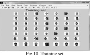
Fig 10 Training set
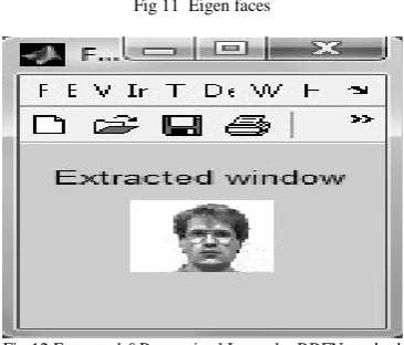
In ORL database 200 images are used as some Training set shown in figure 10 most of them recognized and the result of feature extraction displays the figure 12 .
[image:5.595.49.300.563.705.2] [image:5.595.343.511.688.788.2]Fig 11 Eigen faces
Fig 12 Extracted &Recognized Image by RBFN method
[image:6.595.59.280.280.355.2]The comparison of acceptance ratio , execution time and recognition rates are represented through figure 7,figure8 and figure 9 of graphical method.
Table 2 Comparison of Recognition Rate
Methods Recognition Rate(%)
LDA+Curvelets 98
LDA +Curvelets with RBFN
98.6
The proposed method is compared to LDA+curvelet the recognition rate is increased and it shows to be better than the curvelet+LDA method[10].
Fig 13 Recognition rate
VI . CONCLUSIONS
Face recognition has received substantial attention from researches in biometrics, pattern recognition field and computer vision communities. In this paper, Face recognition using Eigen faces has been shown to be accurate and fast. When RBFN technique is combined with curvelet and LDA, the non linear face images can be recognized easily. Hence it is concluded that this method produces the better recognition rate of 98.6% ,acceptance ratio of 85 % and execution time is only a few seconds. Face recognition can be applied in Security measure at Air ports, Passport verification, Criminal‟s list verification, Visa processing , Verification of Electoral identification and Card Security measure at ATMs.
REFERENCES
[1]. K.Rama Linga Reddy , G.R Babu , Lal Kishore, Larun Agarwal, and M.Maanasa, “ Face Recognition Based on Multi Scale Low
Resolution Feature Extraction and Single Neural Network “
IJCSNS International Journal of Computer Science and Network Security, VOL.8 No.6, June 2008 279.
[2]. S. Lawrence, C. L. Giles, A. C. Tsoi, and A. D. Back, “Face
recognition A convolutional neural-network approach,” IEEE Trans. On Neural Networks, Vol. 8, No. 1 (1997) 98-112.
[3]. Raul Queiroz Feitosa1,Carlos Eduardo Thomaz, Álvaro Veiga, “Comparing the Performance of the Discriminant Analysis and RBF Neural Network for Face Recognition ISAS‟99 – International Conference on Information Systems Analysis and synthesis, Orlando, EUA, agosto de 1999.
[4]. Anupam Tarsauliya, Shoureya Kant, Saurabh Tripathi, RituTiwariand Anupam Shukla , “ Fusion Of Facial Parts And Lip For Recognition Using Modular Neural Network” IJCSI International Journal of Computer Science Issues, Vol. 8, Issue 1, January 2011 ISSN (Online): 1694-0814 www.IJCSI.org 210.
[5] . W. Zhao, R. Chellappa, A, Krishnaswamy, “Discriminant analysis of principal component for face recognition”, .IEEE Trans. Pattern Anal.Machine Intel., Vol 8, 1997.
[6]..Antu Annam Thomas and M. Wilscy “Face recognition using Simplified fuzzy Artmap”Signal & Image Processing : An International Journal(SIPIJ) Vol.1, No.2, December 2010.
[7]. Tolba, El-Baz, El-Harby, “ Face Recognition- A Literature Review”, International Journal of Signal Processing, Vol.2, No.2, 2005, pp.88-103.
[8].Ramesha K1, K B Raja2, Venugopal K “Feature extraction based face recognition, gender And age classification “ International Journal on Computer Science and Engineering,Vol. 02, No.01S, 2010, 14-23.
[9]. Shreeja R “ Facial Feature Extraction Using Statistical Quantities of curve coefficients” International Journal of Engineering Science and TechnologyVol. 2(10), 2010, 5929-5937.
[image:6.595.57.274.395.533.2]