Approximation Behavior of Van der Pol Equation: Large and Small Nonlinearity Parameter

Approximation Behavior of Van der Pol Equation:

Large and Small Nonlinearity Parameter

Behrooz Azarkhalili* , Peyman Moghadas** , Mohammad Rasouli***

Abstract-The labels mathematician, engineer, and physicist have all been used in reference to Balthazar van der Pol.

The van der Pol oscillator, which we study in this paper, is a model developed by him to describe the behavior of nonlinear vacuum tube circuits in the relatively early days of the development of electronics technology.

Our study in this paper will be based entirely on numerical solutions. The rigorous foundations for the analysis (e.g., the proof that the equation has a limit cycle solution which is a global attractor) date back to the work of Lienard in 1928, with later more general analysis by Levinson and others.

Index terms-Van der Pol Equation, Lienard Theorem, Limit Cycle, Two-Timing, Regular Perturbation

I. INTRODUCTION

In the early day of nonlinear dynamic, say from about 1920 to 1950, there was a great deal of research on nonlinear oscillation. The work was initially motivated by the development of radio and vacuum tube technology, and later it took on a mathematical life model of its own. It was found that many oscillating circuit could be modeled by second-order differential equation of the form

      x f x x g x 0     1

Now known as lienard’s equation. It can also be interpreted mechanically as the equation of motion for a unit mass subject to a nonlinear damping force “ - f x x ” and nonlinear restoring force “ -g(x) ”.

In fact lienard equation is equivalent to the system

          _{y g x}x y _{f x y} (2)

The following theorem states that the system has a unique, stable limit cycle under appropriate hypothesis on

f(x) and g(x). (Detail of proof in Jordan and Smith (1978), Grimshaw (1990) and Perko (1991))

*Mathematics Department, Sharif University of Technology, Azadi Ave, Tehran, Iran

**Aerospace Engineering Department, Sharif University of Technology, Azadi Ave, Tehran, Iran

A. Lienard’s Theorem

Suppose that f(x) and g(x) satisfy the following conditions:

1. f(x) and g(x) are continuously differentiable for all x; 2. g(x) is an odd function (or g(-x) = -g(x));

3. g x 0 for 0;

4. f(x) is an even function (or f(-x) = f(x));

5. The odd function F x f u du has exactly one positive zero at x=a, is negative for 0 , is positive and non-decreasing for x and

lim _→∞F x ∞

Then the system (2) has a unique, stable limit cycle surrounding the origin in the phase plane.

B. van der Pol Equation; Fundamental Property In this section we continue the study of the Lienard equation in the special case where f x μ x 1 . This is the van der Pol equation.

Since the van der pol equation which is described by

x μ x 1 x x 0 has f(x) = μ x 1 and g(x) = x so condition 1-4 of lienard’s theorem are clearly satisfied. To check condition (5), notice that

F x μ 1

3x x

Hence condition (5) is satisfied for a = √3, thus van der pol equation has a unique, stable limit cycle. *In fact there is strong theorem about van der Pol equation according dynamical systems theory as follow.

Theorem. There is one nontrivial periodic solution of the

van der Pol equation and every other solution (except the equilibrium point at the origin) tends to this periodic solution. “The system oscillates.”

II. NONLINEARITY TERMS(1) A. Van der pol Equation; Large Nonlinearity Term Consider Van der pol equation

x μ x 1 x x 0 (3)

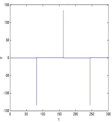
Figure 1. Van der Pol equation, µ=100, extremely slow buildup followed by a sudden discharge

Figure 2. Van der Pol equation, µ=100, extremely slow buildup followed by a sudden discharge

Now consider a typical trajectory in the (x, y) phase plane. The nullclines are the key to understanding the motion. We claim that all trajectories behave like that shown in Figure 3; starting from any point except the origin, the trajectory zaps horizontally onto cubic nullcline y = F(x). Then it crawls down the null cline until it comes to the knee (point B in figure 3), after which it zaps over to other branch of the cubic at C. This is followed by another crawl along the cubic until the trajectory reaches the next jumping-off point at D, and the motion continues periodically after that.

Figure 3. Van der Pol equation, µ=100, typical trajectory in the (x, y) phase plane

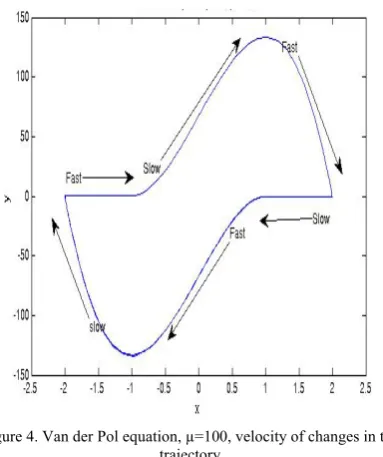
If we go back and look at the Figure 3. again, we will see that the motion is consistent with these ideas. Here is a more detailed description.

We start approximately at x = 2 and y = 0. The system is heavily damped, and there is a kind of creeping motion in which the damping force is balanced by the spring force, very much like a screen door closer. When x becomes less than 1, the damping changes to amplification. The system is rapidly accelerated and passes rapidly through the region from x = 1 to x = -1. When the system reaches the region to the left of x = -1, it is heavily damped, but it now has a lot of inertia. It is rapidly decelerated, and xis approximately -2 when the velocity falls to zero. Then the system creeps back toward x = 0, with damping and spring force in balance. When it reaches x = -1, the amplication begins again and the system is rapidly accelerated from x = -1 to x = 1. At x = 1, the system becomes heavily damped again, but inertia carries it out to about x = 2, where the velocity falls to zero, and the creeping motion begins again.

Figure 4. Van der Pol equation, µ=100, velocity of changes in the trajectory

B. Approximation of Shape and Period of van der Pol Equation; Large Nonlinearity Term

To motivate the new variable, notice that so if we let

w x μF x (4)

Then van der Pol equation implies that

w x μ x 1 x x

Now define new variable y

μ, then (1) and (2) become

x w μF x y

μ x

(5)

Now we want to estimate the period of the limit cycle for the van der pol equation for ≫ 1. The period time T is essentially the time required to travel along thetwo slow branches, since the time spent in the jumps has approximately O( is neglible for large .

By the symmetry, the time spent on each branch is the same. Hence T 2 . To derive an expression for dt, we have on the slow branches, y  F x x x and thus

x 1

But since _μ , finally we have

μ (6)

on a slow branch. So we have T  2 μ dx (7)

*Now we must compute x and x to evaluation of T. for it we note points x and x are maximum and minimum in the figure, so it must be critical points, so must be either vanished or non-exist, but

) 

μ ) (8)

According (8) we must either x= 0 or  ) is non-exist. (Although case of ) = 0 is occurred according Figure 5,

Note that Figure 5 shows only acceptable point is

x 2   x 1    x 2   x 1

Figure 5. x-t diagram and availability of ) Now we can compute T.

T  2 μ dx 2μ x ln  x μ 3 2 ln 2 (9)

Which is O(μ as expected.

The formula (9) can be refined. in fact we show that

T μ 3 2 ln 2 2αμ ⋯ (10)

*Where α 2.308 is the minus of smallest root of Airy function (or Ai (-α) =0 where Ai is Airy function). This correction term comes from an estimate of the time required to turn the jumps and the crawls.

III. NONLINEARITY TERMS(2) A. van der Pol Equation; Small nonlinearity Term Consider the equation of the form

x ϵh x, x x 0 (11)

Where 0 ϵ≪ 1 and h x, x is an arbitrary smooth function. Such equations represent small perturbation of the linear oscillator x x 0 and are therefore called weakly nonlinear oscillator. Two important examples are van der pol equation

x ϵ x 1 x x 0 (12) And Duffing equation

x ϵx x 0 (13)

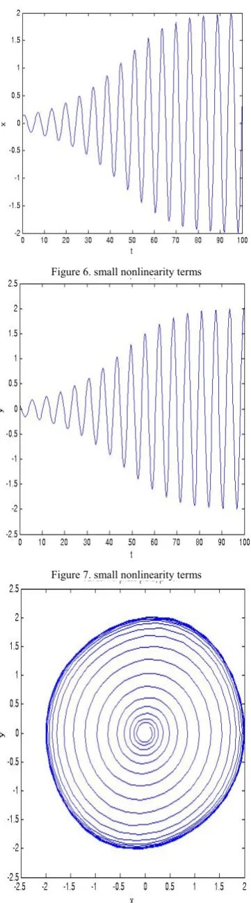
Figure 6. small nonlinearity terms

Figure 7. small nonlinearity terms

Figure 8. small nonlinearity term in x-y diagram

B. Approximation of Shape and Period of van der Pol Equation; Small Nonlinearity Term

*in this section we introduce two methods for approximation of behavior of van der pol equation, then discus on efficiency of each one when time become large and be extended to infinity. In first method we use of regular perturbation and then we use of Two-Timing method for our approach.

B.1 Regular Perturbation Theory and its Failure

As a first approach we seek solution (3) in the form of a power series in ϵ. Thus if x(t, ϵ is a solution, we expand it as

x(t, ϵ = ∑∞ ϵx t (14)

where the unknown function x t are to be determined from the governing equation and the initial conditions. The hope is that all the important information is captured by the first term _ideally, the first two_ and the higher- order terms represent only tiny corrections. This technique works well on certain of problems but it turns in to *trouble here where we handle van der pol equation. To expose the source of difficulties we start with a simple problem that can be solved exactly. Consider the weakly damped linear oscillator.

x 2ϵx x 0 (15)

With initial conditions x(0) = 0, x(0) = 1 *We can easily derived the solution of (15)

x(t, ϵ) = 1 ϵ e ϵ sin( 1 ϵ t) (16)

now we solve the same problem using perturbation theory. Substitution of (14) into (15) yields

x ϵx ⋯ + 2ϵ x ϵx ⋯ + x ϵx ⋯ = 0 (17)

*After ignoring of detail, the solution is (we’re ignoring O(ϵ and higher equations)

x t sin  t

x t t sin  t (18)

Thus

x(t) = sin(t) - ϵt sin(t) + O(ϵ ) (19)

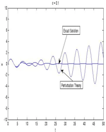
Although two formulas are agree in the following sense: if (16) is expanded as power series in ϵ, the first two terms are given by (19), in fact (19) is the beginning of a convergent series expansion for the true solution, there are two major problems:

Figure 9. the difference between exact solution and perturbation theory B.2 Two-Timing

The elementary note exists about weakly nonlinear oscillation: There are going to be (at least) two time scale in weakly nonlinear solution. We’ve already met this phenomenon in Figure 8, where the amplitude of spiral grew very slowly compared to the cycle time. An analytical Method called Two-Timing builds in fact of two time scales from the start, and produce better approximation than regular perturbation theory. In fact, more than two times can be used, but we’ll stick to the simplest case. To the apply Two_Timing to (1), let τ t

denote the fast order O(1) time and let T ϵt denote the slow time. We’ll treat these two times as if they were independent variables. in particular , function of the slow time T will be regarded as constant on the fast time scale τ .

Now we can turn to mechanics of method. we expand the solution of (1) as a series

x t,ϵ x τ, T ϵx τ, T O ϵ (20)

The time derivates in (1) are transformed using the chain rule:

x   _{τ   τ τ} ϵ    (21)

A subscript notation for differential is more compact, thus we write (20) as

x ∂τx ϵ∂ x (22)

After substituting (20) into (22) and collecting powers of ϵ, we find

x ∂τx ϵ ∂τx ∂ x O ϵ (23) Similarly,

x ∂_ττx ϵ ∂_ττx 2 ∂_τ x O ϵ (24)

To demonstrate the power of this method, first apply it to

Collecting powers of ϵ yields a pair of differential equations:

O 1 : ∂_ττx x 0 (26)

ϵ : ∂_ττx 2 ∂_τ x 2 ∂_τx x 0 (27)

As same as regular perturbation theory, we can solve (26) and (27) and we get

x τ, T e τsin  τ (28) Hence

x= e τsin τ O ϵ (29)

is the approximate solution predicted by Two-Timing . Figure 10. compares the Two-Timing solution (29) to the exact solution (7) for ϵ 0.1 . The two curves are almost indistinguishable ,even though ϵ is not terribly small. This is a characteristic feature of the method- it often works better than it has any right to.

If we want to go further with this problem, we could either solve for x and higher order corrections, or introduce a super-flow time ϵ t to investigate the long term phase shift caused by the O ϵ error in frequency.

Figure 10. the difference of exact and two timing method

The equation is x ϵ x 1 x x 0 . Using (23) and (24) and collecting powers of ϵ, we find the following equations:

O 1 : ∂ττx x 0 (30)

ϵ : ∂_ττx x 2 ∂_τ x x 1 ∂_τx (31) The O 1 equation is a simple harmonic oscillator. Its general solution can be written as

x r T cos  τ φ T (32)

Where r T and φ T are the slowly-varying amplitude and phase of x .

To find equation governing r T and φ T , we insert (32) into (31). this yield

φ . Some terms of this form already appear explicitly in (33). But-and there is also important point- there is a resonant term jurking in sin τ φ cos τ φ ,because of the trigonometric identity

sin τ φ cos τ φ sin τ φ sin  3 τ φ (34)

after substituting (34) into (33), we get

∂_ττx x 2r′ r r sin τ φ

2 φ′ _{cos τ φ r sin  3 τ φ (35)}

To avoid secular term, we require

2r′ r r 0 (36)

2 φ′ _{0 (37)}

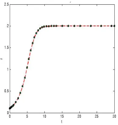
First consider (36). It may be rewritten as a vector field

r′ r 4r (38)

On the half line r 0. Since r∗ _{0 is unstable fixed}

point and r∗ _{0 is stable fixed point, lim}

→∞r T 2.

Figure 11.radius of limit cycle

Secondly (37) implies φ′ _{0 so φ T φ for some} constant φ . so lim _→∞x τ, T 2cos τ φ ) and therefore

lim_→∞x t 2 cos t φ   O ϵ (39)

Thus x t approaches a stable limit cycle of r 2 O ϵ .

To find the frequency (and therefore period) implied by (39), let θ t φ T denote the argument of the cosine. Then the angular frequency ω is given by

ω θ 1 φ 1 ϵφ′ _{1 (40)}

through first order in ϵ. Hence ω 1 O ϵ ; if we want an explicit formula for this O ϵ correction time, we’d need to introduce a super flow time ϵ t .

IV. CONCLUSION

*In this paper we study van der Pol equation which is an important nonlinear ODE. Then we study behavior of it for very large and very small nonlinearity parameter in this equation and approximate some property of it such as period and frequency and radius of limit cycle. In addition, we can improve these approximations by using of more terms in regular perturbation methods or using of super flow time in Two-Timing method to achieve better approximation.

REFRENCES

[1] L. Perko, Differential Equations and Dynamical Systems, 2nd ed., Springer, New York, 1996.

[2] J. Guckenheimer and P. Holmes, Nonlinear Oscillations, Dynamical Systems, and Bifurcations of Vector Fields, Springer, New York, 1983.

[3] A. Gray, M. Mezzino, and M. A. Pinsky, Introduction to Ordinary Differential Equations with Mathematica.

[4] J. Palis and W. de Melo, Geometric Theory of Dynamical Systems, Springer, New York, 1982.

[5] F. Verhulst, Nonlinear Differential Equations and Dynamical Systems, Springer, Berlin, 1990.