Robust methods of analysing repeated measurements data
in a longitudinal setting.
SHANBHAG, Sharayu.
Available from Sheffield Hallam University Research Archive (SHURA) at:
http://shura.shu.ac.uk/20352/
This document is the author deposited version. You are advised to consult the
publisher's version if you wish to cite from it.
Published version
SHANBHAG, Sharayu. (1999). Robust methods of analysing repeated
measurements data in a longitudinal setting. Masters, Sheffield Hallam University
(United Kingdom)..
Copyright and re-use policy
Fines are charged at 50p per hour
~ 7 APR 2003 4 ' . lb
-
8 m
2004
% p n
1 U t-t« 2GQ5
f'S
1 1 MAY 2006
Cp ,,
ProQuest Number: 10700998
All rights reserved
INFORMATION TO ALL USERS
The quality of this reproduction is dependent upon the quality of the copy submitted.
In the unlikely event that the author did not send a com plete manuscript and there are missing pages, these will be noted. Also, if material had to be removed,
a note will indicate the deletion.
uest
ProQuest 10700998
Published by ProQuest LLC(2017). Copyright of the Dissertation is held by the Author.
All rights reserved.
This work is protected against unauthorized copying under Title 17, United States C ode Microform Edition © ProQuest LLC.
ProQuest LLC.
789 East Eisenhower Parkway P.O. Box 1346
ROBUST METHODS OF ANALYSING
REPEATED MEASUREMENTS DATA IN A
LONGITUDINAL SETTING
ROBUST METHODS OF ANALYSING REPEATED
MEASUREMENTS DATA IN A LONGITUDINAL SETTING
Sharayu Shanbhag
A thesis submitted in partial fulfilment of the requirements of
Sheffield Hallam University
for the degree of Master of Philosophy
TABLE OF CONTENTS
Abstract
.. 1
Pase
Introduction
... 2-6
Chapter 1:
Repeated Measures Data Structures and
Collection
... 7-18
1.0
Introduction
... 7
1.1
Repeated Measures Data Structures
... 8-9
1.2
Problems with Data Structures
... 9-12
1.3
Obtaining Repeated Measures Data
... 12-18
1.4
Aims of Any Repeated Measures Data
Collection and Analysis
... 18
1.5
Overview
... 18
Chapter 2:
Data Analysis and Assumptions
... 19-44
2.0
Introduction
... 19
2.1
Assumptions about the Distribution of the Data
... 20-27
2.2
Methods of Analysis
... 28-32
2.3
Testing
... 32-35
2.4
Modelling
... 35-39
2.5
Discussion
... 39-42
2.6
SAS Procedures Used
... 43
2.7
Overview
... 44
Chapter 3:
The Observed Data and Basic Summary
Measures
... 45-54
3.0
Introduction
... 45
3.1
Observed Data Structures
... 45-49
3.2
Classification of Vital Signs Data
... 49-51
3.3
Univariate Summary Measures
... 52-53
3.4
Overview
... 54
Chapter 4:
Exploratory Data Analysis
... 55-82
4.0
Introduction
... 55
4.1
Profile Plots of the Continuous Data Over Time
... 55-59
4.2
Missing Data Records Over Time
... 60-61
4.3
Distribution of the Continuous Data Over Time
... 62-70
4.4
Plots of Summary Statistics by Treatment Over
Time
... 71-76
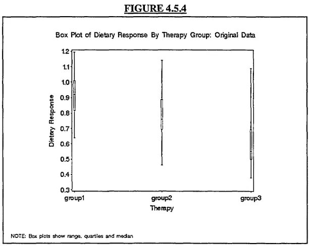
4.5
Distribution of Continuous Overall Data Per
Group
... 77-79
4.6
Categorical Approach: Frequency of
Abnormally High Results at Each Time
... 79-80
TABLE OF CONTENTS (CONTINUED)
Page
Chapter 5:
Univariate Summary Measures Analysis
•••83-111
5.0
Introduction
...83
5.1
Continuous Data Analysis: Response Features
84-100
Analysis
5.2
Categorical Data Analysis
...101-110
5.3
Overview
...111
Chapter 6:
Data Reduction
•••112-140
6.0
Introduction
112-113
6.1
Multivariate Normality
...113
6.2
Reducing the Data Sets
...113-114
6.3
Structures of Reduced Multivariate Data
...114-116
6.4
Univariate Methods for Comparison of
116-117
Reduced Data With Original Data
6.5
Univariate Analysis for Each Reduced Data
117-132
Point
6.6
Univariate Summary Measures for Reduced
133-139
Data
6.7
Overview
...140
Chapter 7:
Multivariate Testing
•••141-147
7.0
Introduction
141
7.1
Methods
142
7.2
Results
143-147
7.3
Overview
...147
Chapter 8:
Parametric and Non-Parametric Modelling
• ••148-170
8.0
Introduction
148
8.1
Categorical Data Analysis
...149-154
8.2
Continuous Data Analysis
...155-168
8.3
Overview
...169-170
Chapter 9:
Overview
171-173
9.1
Discussion and Conclusions
171-172
9.2
Further Work
...173
References
174-177
Appendices
1-105
A
Tables
1-67
ACKNOWLEDGEMENTS
I would like to extend my thanks to my supervisors Prof. Kanji and Dr. Fosam for
their advice and suggestions during the preparation of this thesis. I would also like
to thank my previous company SANOFI Inc. and Dr Roy Saunders for providing me
with the analysis data sets and the computing resources to conduct this study.
Finally I would like to thank both my parents and husband for their help and
DECLARATION
I declare that the following dissertation embodies the results of my special study,
that the dissertation is my own composition, and that it has nor previously been
ABSTRACT
Two longitudinal data sets were individually analysed within this thesis. Data set A was a vital signs data set and data set B was a data set of dietary response. Initially, an exploratory data analysis approach was used to analyse the data at each univariate time point. Missing data were observed and an approach was suggested of estimating some of these missing records. It was found that this missing data only affected multivariate test results when the proportion of individuals with missing records was large. While using the conventional methods of analysis of the data set as a whole, some authors suggest using restrictive covariance structures corresponding to the data, following the assumption of normality. An issue that can cause problems with matrix calculations for any multivariate method and therefore invalidates the multivariate procedures is if the number of repeated measures is greater than the number of individual profiles per group. In this situation there is the problem in assuming a normal distribution for the data, which is a major assumption for any multivariate analysis, when this assumption does not really hold. The main aim of our research was to devise methods of analysing the whole data set when the data is of the form mentioned above and when the assumption of normality fails. Various data reduction approaches were suggested for analysing the data in a multivariate manner for this situation. The following three approaches were suggested to reduce the number of repeated measurements: (a) multivariate summary measures, (b) principal components and (c) averaging the data over groups of time points.
Both the principal components and summary measures approaches do not retain the time element and so firm conclusions can not be made. Our main contribution, within this thesis, is to illustrate that there are ways of reducing the data by still retaining the element of time in some manner. This is by using the method of averaging the data over groups of time points. The suggested procedures, of averaging data over segments of time, allows the use of the usual multivariate tests and modelling procedures without having to meet the assumption of normality or having any constraints on the covariance structure. This reduction method leads to more robust tests. Most analysis of variance tests become reduced to Chi- squared tests following this type of data reduction approach.
INTRODUCTION
So far in the literature to date there have been a vast number of methods and applications used in the
analysis of repeated measures data. The topic of ‘Repeated Measures Data Analysis’ is an expanding
field and one in which there is a range of both new and old literature. There is also a wide variety of
varying opinion on the way that repeated measures data should be analysed. Hence, it is not possible to
compile a summary based on just methods used in literature so far. Instead, our research looks into
some of the most common methods of analysis of repeated measures data (particularly for longitudinal
research) which have been suggested until now. We look into some of the available literature in the areas
of ‘repeated measures’ and ‘profile data’ analysis with particular attention focussed on the sorts of data
obtained from ‘longitudinal trials’. In our research we will be looking at biomedical data. However,
repeated measures data can also arise in a wide variety of other contexts. Other research areas include
agricultural, psychological, economic and social research.
Chapter 1 describes clearly what repeated measures are, shows the general structure of a longitudinal
data set and suggests ways of obtaining such data. Both an ideal situation and a messy situation are
described in order to give an idea of the shortcomings of such data. Specifically mentioned are the
problems of missing data, unscheduled visits, non-balanced data, early dropouts and unequal spacing
between visits. Ideas are suggested on how to control some of these problems but it must be noted that
some of these suggestions are not always practical. Details are given on study design used to obtain
repeated measure data. Through our research we have discovered that there are three general methods of
collecting any type of data. These are through setting up a designed experiment, conducting a survey or
with an observational study [40]. All three methods mentioned are very different in their approaches.
However, the information being gathered using any of these methods would be similar whichever is
used. The choice of using a particular method is up to the individual carrying out the study or the
investigator. Factors, which may affect the choice of designs, would be things such as cost, efficiency,
convenience and availability. It is believed that repeated measures data are usually obtained via some
type of designed or planned experiment. There are four study designs that specifically lead to the
measurement of repeated measures datal36]. These are split plot designs, crossover studies, source of
variability studies and longitudinal studies. A study using any combination of these four designs would
Chapter 2 reviews some common methods used to analyse repeated measures or particularly longitudinal
data. Distributional assumptions are also described in this chapter.
Chapter 3 describes the two longitudinal data sets A and B. Data set A was a ‘large’ longitudinal
unbalanced data set which had three variables (Heart Rate, Systolic Blood Pressure and Diastolic Blood
Pressure) that were measured for 86 patients who were from 2 centres and were each randomly allocated
to one of four treatment groups (1 to 4). The three vital signs were each measured at multiple time
points (at baseline and then over 24 hours at hourly intervals) per individual using an ambulatory
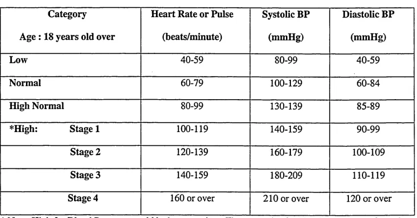
measurement device. Normal ranges for vital signs and other categories were obtained from National
Blood Pressure Education Program, JNCV Report and also from private communication with an M.D
[69]. These categories were used to further classify data set A to obtain a categorical data structure. Data
set B was a ‘small’ longitudinal balanced data set measured for 24 individuals that were randomly
allocated to one of three diet groups (1 to 3). The readings were taken at baseline and also at 9 other on
therapy time points. This data set had no categorical information available. These two data sets A and B
were each analysed in an appropriate manner.
In the past, it has been recommended to use individual univariate tests at each time point to avoid the
difficulties associated with multivariate analysis methods due to the fact that they can at times become
quite tedious or complicated. Nowadays, with computers and computer packages such as SAS and S-
Plus etc., the issue of problems with computation of multivariate methods is not of so much of a problem
as it was in the past. In the existing literature many authors I19,30] disregard these univariate methods
over time, claiming that they are not worth while. This is mainly because of dependence between
successive measurements and difficulty in interpreting the various individual test results. Only the
univariate approach of ‘Response Features Analysis’ is a method that is still considered to be worthwhile
by various authors 119,20,43J. It was therefore decided to use only this univariate approach to summarise
the data over time.
Initially an exploratory data analysis was conducted on the data and these findings are displayed in
chapter 4. There was the problem of missing data that was encountered during data analysis. Thirteen of
the 86 records from data set A and 4 of the 24 records from data set B had at least one missing ‘on
treatment’ record. Section 4.2 briefly introduces the reader to the area of missing data, suggests some
commonly used methods and describes an ad-hoc missing data generation process that was devised, to
obtain a data set that contained 84 records of complete ‘on treatment’ information with 2 patients still
having missing baseline information. It was felt that data generation was reasonable for data set A since
it was very large and the time points were close together and there were many time points for each
patient. It was believed that losing 2 patients worth of data out of 86 records at the start of the study
would not affect the results that drastically for any univariate or multivariate time dependent methods
applied to this particular data set. When analysing the smaller data set B, only 4 of 24 individuals had at
least one missing record. Following the data generation method, there were 22 individuals remaining
with a full set of records but the data set would now become unbalanced. Since the data set was smaller
than data set A and the time points were further apart, we were uncertain of whether the data generation
method would be appropriate for data set B.
In order to get a feel for what was going on with the data and how the data generation method would
affect any results, both the old data sets (with missing records) and the new data sets (with generated
observations) were looked at carefully and the results compared. For this reason, even though not first
planned, separate univariate tests were conducted on the individual time points, using both the original
(with missing records) and the complete (generated) data sets, as a means of comparing methods only.
This approach was also applied to the summary measures from the original and the complete data sets
and these results were also compared. These methods were conducted on both data sets A and B. There
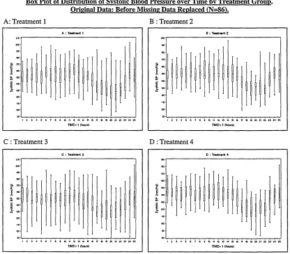
were no vast differences between the results before and after data replacement. Due to the similarity of
figures produced before and after data replacement, only those using the data set with missing records
are displayed, to show the behaviour of the data across or over time.
In analysing both data sets A and B, it was decided to analyse the data using multivariate testing and
mixed modelling techniques, since this is one of the most efficient methods of dealing with repeated
measures data. Of the various SAS procedures of conducting multivariate-modelling techniques, there
are two commonly used procedures in dealing with modelling continuous data. These are Proc GLM
and the more recent method of Proc MIXED. Details on these and other SAS procedures used in the
analysis of the data for this thesis are described in section 2.6.
After gaining a general feel for the topic, it was found that when most multivariate repeated measures
data analysis are conducted, various assumptions (including normality, equal correlation between groups
and equality of variance) need to be made about the distribution of the data for the tests to be valid.
multivariate analysis of variance, there are still occasions that problems can occur with multivariate
analysis of variance (MANOVA). A specific case is when there are more repeated measurements than
the number of individuals within a groupl27,35] and hence normality of the data may not be a reasonable
assumption. This happens to be the case for both data sets A and B.
The main purpose of our research is to see what happens if the usual assumptions of normality is not
met. Some methods from the literature, that are used to analyse this form of data, when these general
assumptions are not valid, are looked at and finally some alternative ideas are suggested to those used in
practice. A suggestion to overcome this problem as mentioned in the literature, was ‘Response Features
Analysis’ or the ‘Summary Measures’ (S.M.) approachl24,431. The approach was for one single summary
measure to represent the whole profile for an individual. This summary measure would then be analysed
using some univariate testing method such as the parametric analysis of variance (ANOVA) or non-
parametric Kruskal-Wallis test (for comparing more than two treatments). Chapter 5 describes the
results obtained from analysing the data using this S.M. approach. The disadvantage is that multivariate
methodology gets lost in using this procedure.
The approach of dealing with multivariate data with the problem of having more measurements than
individual profiles has not been greatly focused on in the literature. For this thesis, it is suggested that
the best method of dealing with the data, so a robust multivariate analyses could still be conducted, was
a segmentation of the data with data reduction of some kind. Chapter 6 gives details on suggested
approaches for data reduction in order for a valid multivariate approach to be applied. Three methods of
data reduction were looked into. One of the methods was an extension of the S.M approach using a set of
6 summary measures (mean, median, min, max, ql and q3) together to describe each individual profile.
These data were then analysed in a multivariate rather than univariate fashion. The second approach,
was an extension of the idea mentioned by Jones and RiceI33] who used P.C.A to reduce the number of
individual profiles. The approach used in this thesis reduced the number of time points instead of the
number of individual profiles. The final approach, which was suggested for the purpose of this thesis,
was to use the mean of every two (for data set A only) or three (for both data sets A and B) observations
instead of each time. This method yields a data set that still preserves a time element whereas the other
two methods do not maintain this factor. Multivariate tests were conducted to see whether the three
approaches give similar results or whether one approach is better than another. All multivariate test
obtained whichever method was applied and whether missing data would be an issue for multivariate
testing. The multivariate method of Mahalanobis distances was used to test for treatment differences for
all the above mentioned data sets. The results from each of the multivariate tests were then compared
and these are shown in chapter 7. Multivariate testing was affected by missing data since records were
not retained during analysis.
All multivariate mixed modelling procedures were conducted on both the original data before imputing
missing records and also on the reduced data obtained from the complete data set (after data generation)
to maintain consistency with the multivariate tests that were previously conducted. It was, however, not
necessary to work with a complete data set since Proc MIXED is not affected by missing data. The
procedure was applied to only the reduced data, using the reducing procedure of averaging over
segments of time, since this was the only reduction approach that retained the element of time as with
the original data. This allowed a comparison of results before and after data reduction. Chapter 8 shows
the findings of the mixed modelling approach. Each of the variables after being reduced by averaging in
groups of three measurements (or two measurements if possible) were modelled using a mixed
modelling approach after adjusting for baseline reading and time. Individuals were modelled as random
effects in the models. No conclusions could be drawn about any other reduction methods since time was
lost in the calculations.
From conclusions described in chapter 9, it was found that the data before and after imputing missing
information gave similar findings. The best data reduction approach appeared to be the summary
measures (SM) approach for testing the data and also the grouped mean (method 1) for modelling the
data. Details of further work are also discussed in this chapter.
In conducting the initial exploratory analysis, there were some problems and issues that were
encountered. Some of the main issues that led to problems during the analysis of this data set were
missing observations and imbalance between treatment groups. Missing data was not an issue when it
came to analysing data in a univariate manner. The problem occurred while conducting any multivariate
methods (P.C.A. and Mahalanobis Distance) on the data set with missing information, especially if there
were many individuals with missing data. One of the most up to date approaches of modelling such data
CHAPTER 1: Repeated Measures Data Structures and Collection
1.0 Introduction
The subject of ‘Repeated Measures Data Design and Analysis’ is a very broad research area. Wishart
(1938)1621 and Greenhouse and Geisser (1959)[27j conducted some of the earliest research in this field. It
is only in the recent years (since 1980) that the area has become very popular and the field is still
growing to this date. Among the various books published in the area, Crowder and Hand [14,30], Diggle,
Liang and Zeger[18] and Vonesh and Chinchilli[61] are among the most popular and up-to-date ones. All
of these books were published in the late 1980’s to mid 1990’s. These books and references therein will
give the reader a broader insight into the topic of research and may enlighten as to the variety of both the
old and new literature available and the various works that have been conducted in this field. There have
been a variety of works published in the area of ‘Repeated Measures Data’. There is still, however, a
large potential for other research ideas in the spectrum of research readily available.
Repeated measures data can arise through various experimental designs including spilt-plots, cross-over
trials and parallel groups design experiments but to name a few [36]. For the purpose of this thesis, only
repeated measures data from a longitudinal setting will be focused on. The terms ‘Longitudinal Data’ or
‘Repeated Measures Data’ will be used interchangeably to refer to the data used during analysis.
The present chapter introduces the reader to repeated measures data structures and collection. The
structure of specifically a longitudinal data set in both an ideal and a messy situation are described in
section 1.1. Some of the shortcomings of repeated measures data, as described in section 1.2, include
the problems of missing data, unscheduled visits, non-balanced data, early dropouts and unequal spacing
between visits. Another issue, which is to be the main area of focus for this thesis, is when the repeated
measures are large compared to the number of individuals on whom they are measured[27,35]. Ideas are
suggested on how to control some of these problems but it must be noted that some of these suggestions
may not sometimes be applicable. Section 1.3 gives details and examples of study designs used to
obtain repeated measure data. Section 1.4 explains the main reasons for collecting this type of data and
mentions some questions that may be asked during the data analysis stage. An overview of this chapter
1.1 Repeated Measures Data Structures
This chapter is intended to give the reader an introduction to repeated measures data structures.
Below is a description of what repeated measures data actually are and how these types of data are
obtained. Repeated measures data are multiple recordings of an observational unit or the same dependent
variable, (e.g. blood pressure, heart rates or some other measurement), which are taken for each of a
number of individual experimental or primary sampling units (e.g. patients, subjects or some other
individuals). The experimental units are randomly selected to represent various strata or are randomly
assigned to levels of a grouping factor (e.g. therapy, treatment or some other group). In other words, an
individual can either be allocated to one of several groups or can fall into one of a number of naturally
occurring groups. The responses that are being measured under the various conditions are the
observational units and these can be taken (or measured) at various points in space or time. In our
research, we will be looking at biomedical data. However, repeated measures data can also arise in a
wide variety of other contexts or research areas such as agricultural, psychological, economic and social
research.
Initially an important thing to remember is that ‘Repeated Measures’ are the type of data, not the design
of experiment, which is a mistake that is often made. The terminology that is often used to explain the
set of multivariate repeated measures data for an individual unit is an individuals profile. This can be
seen more clearly in the diagram below which shows data collected in a longitudinal manner in an ideal
situation.
Example 1: An Ideal Situation:
Re p e a t e d Re a d in g s o ft h e Sa m e Re s p o n s e Va r ia b l e
Group 1
Unit 1 X X X X X X X X X X
Unit 2 X X X X X X X X X X
Group 2
Unit 3 X X X X X X X X X X
Unit 4 X X X X X X X X X X
i
1---1---1--- 1---r ---1---1---j---1
tl h t3 U ts t$ t7 tg t9 tjo
Times of Readings (Days)
each of these individuals at the same time points (k=l to 10). The ten time points are equally spaced
apart. There are no missine data in this example and the data are balanced between groups. Hence this
is repeated measures data from a ‘balanced complete longitudinal’ design. The general notation for any
individual observation using the information from above would be Yjjk. So, for example, the individual
observation unit 3 at time 3 from group 2 would be shown by Y213.
Note: As can be seen in the example above, in an ideal world it would be preferable for each sampling
unit to have measurements at the same times and also for there to be equal spacing between each pair of
response measurements or readings. Another thing that is preferable is the complete collection of data.
However it is not always possible in most real situations for us to meet all the criteria mentioned above
while collecting data and there usually tends to be a shortcoming in at least one of the conditions
mentioned above. The diagram below shows some of these shortcomings in a clearer fashion for
longitudinal data collected in a messy situation.
Example 2: A Messy Situation
Group 1
Unit 1 X X X X X X X X X X
Unit 2 X X X X X X X X X
Group 2
Unit 3 X X X X X X X
Unit 4 X X X X X X X X X X
Unit 5 X X X X X X X
1
ti
1
h
1
t3
1
u
1
t5
1
u ■1 1
h t8 1
t9
1
tic
Times of Readings (Days)
1.2 Problems With Data Structures
Data structure problems can lead to problems during analysis. Some of these problems are mentioned
below and are illustrated in Example 2 above:
a) Unequally spaced time points between measurements.
In the situation above, the design is such that the data measurement is not at equally spaced time points,
The main reason for this could be due to the fact that measurements can only be taken at certain times
because of external or environmental factors. An example would be if it were known, before the study
began, that there were specific times that the outcomes of interest would occur and these would be the
also occur in a designed experiment with equally spaced time points when there are unscheduled visits.
The main difference is that for the designed experiment the additional set of information could always be
dropped for analysis purposes. However, if the study was set up to measure data at unscheduled visits
this could not be done. It must be noted, however, that it is not always practical to set up an
experimental design with equal spaced time points, especially if the variable being measured is only
available at certain times. In this case, an appropriate method of analysing the data would be using a
time series approach.
b) Unscheduled visits.
There is one extra reading for unit 4 that is measured at an unscheduled visit between t5 and t$. This
would mainly be due to the availability of the sampling unit. For example, a patient knows that he or
she can not make their next appointment and therefore turns up early to tell the doctor of the situation.
The doctor still takes measurements in the hope that the data can be used. Even though it is not
planned, it is sometimes believed that partial data is better than no data at all. If the study were a
designed experiment with equal spacing between measurements, there would be justification in
removing any additional data especially when they were unscheduled measurements. For a design that
has unequal spacing between measurements the process of removing additional data would not be
justifiable. This data should then be analysed as a data series again using time series techniques.
c) Incomplete / Missing data at scheduled visits.
Sampling units 2, 3 and 4 all have missing readings that were supposed to be measured at scheduled
visits. The main reasons for this could be that the equipment being used to measure the data fails or that
the sampling unit might not be able to make the scheduled appointment. Both a designed experiment or
a study that is not designed could yield missing data and it is believed that this is something that can not
readily be controlled whatever the design is. Having one missing record for a patient would force the
whole observation to be dropped when most multivariate methods are applied to the data. This means
that a lot of useful data is wasted. The solution in this case is to generate these missing data in some
way, if possible.
d) Unbalanced data between groups.
It can be seen that group 2 has one more patient than group 1. This is an issue that causes problems in
some analyses. The main way that this problem can be solved is by conducting a designed experiment.
there are times that patients drop out of a study directly after randomisation and hence there are different
numbers of observations in each treatment group. It is believed that a designed experiment may have
greater control over this issue than any other type of study. Depending on the size of the study and the
numbers of patients within different groups, it is suggested that the data set could be made to balance by
randomly dropping the extra data. Note that, this suggestion is only deemed to be appropriate if the data
set is large enough as the loss of a small number of observations is not expected to affect the results
greatly. For example, if there were either 21 or 22 individuals in each of 4 treatment groups and if the
data set was forcibly balanced, for both treatment groups and centre, then one would end up with 20
individuals in each treatment group.
e) Early Termination
As for unit 5, a patient can drop out of the study before the scheduled time of completion. This means
that the sampling unit does not have a full set of records. This is an issue that can not be controlled
based on the design of the study. These observations would generally be dropped from any usual
multivariate analysis on the data.
Another problem, which is to be a part of the main focus for this research, is as follows:
f) Number of Individuals are less than the Number of R.M.
When the number of repeated measures is greater than the number of individuals then there are problems
in calculating the sums of squares (SS) and degrees of freedom (df) while conducting multivariate
ANOVA [27]. When p is large compared to the number of residual df, a singular variance-covariance
matrix is estimated and this in turn means that the MANOVA test statistic can not be defined [35J.
A practical argument for explicit modelling of the covariance structure, as was stated by Diggle, Liang
and Zeger[18] concerns the number (p) of repeated measurements per experimental unit. It was observed
that when p is large, the objection to estimating p (p+l)/2 parameters in the covariance structure gains
force since this expression is of the order of p2. In extreme cases, p can also exceed the available
replications.
A different problem also arises if the number of individuals is not considerably greater than the number
of repeated measures. In this case, in most situations, the assumption of normality or having tests as in
the case of normal distributions would not be reasonably valid. Hence a suggestion would be to reduce
the number of repeated measurements in some intuitive manner in order to have the validity of the model
reasonable question may be: ‘Would all of the many repeated measures be of relevance or could a fewer
number of measurements give the same results as all observations?’
1.3 Obtaining Repeated Measures Data
1.3.1: Data Collection
Generally, most data sets are obtained by one of the following three methodsl40]. All three types of data
collection mentioned are very different but they all use very similar statistical notation in that they all
have ‘factor’, ‘level’ and ‘effect’:
A) Designed Experiments
As the name suggests, a designed experiment is planned or designed before the study takes place.
Example:
Experimental units (patients) are randomly assigned to one of four groups (drugs 1-4). After the experimental units are assigned to their groups, responses (heart rates) are measured.
For this designed experiment, therapy would be a ‘factor’, and each drug would be a ‘level’ within the
factor. Each level would have an ‘effect’ on heart rate. So applying any one of the drugs has an effect on
the heart rate of the patient.
B) Sample Surveys
A survey design is a plan that is used to collect data on the sampling units but treatments are not applied
to these units. The sampling units are usually people and they already have certain pre-existing
attributes e.g. age or qualifications. The data to be measured could be a variable such as salary and this
can be determined for each individual sampling unit.
Example:
A survey could be taken on a set of individuals to see how individual salaries behave based on qualifications.
For this survey, qualifications would be the ‘factor’, and each ‘level’ (A, B) of the factor would have an
‘effect’ on salary. Note, a particular qualification would not cause the level of the salary but people with
C) Observational Studies
The sampling units here already exist before data is collected and they are not from a planned study.
Example:
Patients visiting a doctor’s office at the time of visit have their weights measured and they are categorised into groups based on this information. The blood is then tested for levels of cholesterol.
For this observational study, weight would be the ‘factor’ and each weight measurement would be a
‘level’ of the factor. Differences in the cholesterol level between the diagnostic groups would be
‘effects’ of the factor levels.
1.3.1.1 Choice of Data Collection Method: In General.
A question now is ‘which type of design should be used in general?’ It is usual for the experimenter to
go with the most convenient method of data collection based on certain external factors that can not be
controlled. The person conducting the study should decide based on the following factors before they
begin data collection:
1. The aim of the project.
A survey could be looking into specifically a small population, such as of an ethnic origin, since it is
of interest. This, in turn, could lead to a smaller sample size than one would actually prefer and so
could lead to problems with data analysis. If the study is observational in nature, then the
investigator has no choice than to go with what is available. A designed experiment is usually the
best way of controlling the data obtained.
2. The cost of the project.
If fewer financial resources are available than are required, this could again influence the amount of
data collected. A designed experiment is often more expensive to run than an observational study or
a survey.
The points mentioned here may be obvious but can often get overlooked. The aim would be to set up a
design, which captures exactly what the experimenter wants, before starting to collect the data. If the
data can be obtained through a designed experiment, then this is recommended since it is believed that
1.3.1.2 Choice of Data Collection Method: For Repeated Measures Data.
Specifically with regards to longitudinal data, two important issues that lead to problems with data
analysis are of missing data and early termination. Neither problem can be controlled by study design.
Conducting a designed experiment or survey can usually control the problems of unequal spacing
between time points and unscheduled visits. This is not true when the variable being measured is
restricted to certain times of measurement, as in an observational study or a study of convenience, where
there would be no solution to this problem. Unbalanced data can be controlled if a balanced study
design is conducted with no dropouts.
Hence, it is suggested that the best way of obtaining repeated measures data, that in the end will be
easier to analyse, is to obtain the data using a designed experiment or survey. A number of factors need
to be taken into account when collecting data such as the aim, cost and efficiency. A designed
experiment or survey does not control factors such as malfunction of a machine used to measure the
variable of interest, early termination from the study or other environmental factors. It should be noted
that once it is decided to obtain the repeated measurements for a particular variable then the data design
usually ends up falling into the category of a ‘designed experiment’. This is the case whichever initial
method was used to classify the observational units into experimental groups. There is usually some sort
of planning in the process of collecting repeated measures data. It should be noted that the data sets that
are to be used for this thesis are from designed experiments.
There are various standard designs for experiments that fall into the category of a “designed experiment”
and a detailed explanation of these can be found in various texts. Due to time constraints, further details
of designed experiments will not be given in this thesis. The reader can refer to any books with
‘Experimental Designs’ or ‘Designed Experiments’ in the title and any references therein [12,44,641.
Further details are given below on the designs used to obtain repeated measures data in particular.
1.3.2: Designs Used to Obtain Repeated Measures Data
Many different designs can be used to obtain repeated measures data. Experimentation and collection of
repeated measures data are very important since the collection of such data particularly allow
comparisons of treatment effects over time. There are a wide variety of study designs that can lead to
the collection of repeated measures information. Of these, the four most important study designs are
longitudinal, source of variability, crossover, and split-plot studies. A combination of any two or more
individual unit is observed under two or more conditions. Koch 1361 gives a good overview together with
references for all four designs with some examples of each and also some statistical methods and
applications particularly in reference to split-plot designs. The advantages and disadvantages of each
design and similarities and differences between them are also mentioned.
We will begin by giving a brief example of each of the four designs with a brief overview of similarities
between the design structures and any important points of discussion. The main body of the report will,
however, focus on repeated measures from a longitudinal study, and the analysis of such data.
A) Split-Plot Experiments:
Example:
Sixty-four laboratory rats are randomly divided into four groups o f 16. Each group of 16 is assigned to a block of 4 cages (with 4 rats in each cage). Four dietary calcium sources are randomly assigned to the four cages within each block. Four rats are assigned to each cage. Four implants (A, B, C ,D) are randomly assigned. [Littell [701].
Split-plot designs have differences compared with other designs in that they have more than just one
stage of randomisation. Subjects are initially randomly assigned to treatment groups or selected from
strata. Conditions are then randomly allocated within these groups or strata.
Treatment groups can be based on a single factor or on a cross-classification of two or more factors.
They can be assigned to whole plots based on a completely randomised, a randomised complete blocks
or a type of incomplete blocks design. Conditions can similarly be assigned to split-plots.
These designs are commonly used in agricultural experimentation, where the subjects are whole plots or
fields within which split-plots are the observational units.
B) Cross-Over (or Change-Over) Designs:
Example:
Each subject is randomly assigned to either sequence AB or sequence BA. Responses to each successive treatment are measured for an allocated period. The conditions are the time periods and treatment and also the proceeding treatment.
The subjects within a crossover design are randomly assigned to treatment groups or are selected from
strata. They are randomly assigned with alternate treatment sequences. One could seek here estimation
For a cross over study, the previous treatment can influence the response on a particular treatment and so
a carry over or residual effect may occur. If it is known that the extent of carry over is more than
negligible then some sort of adjustment is needed. It has been suggested that sequences should be
devised to allow estimation of location, treatment and carry-over effects. This at times can be hard to
implement. An alternative design where each subject gets only one treatment eliminates this problem.
C) Source of Variability Studies
These studies identify the amount of variability between responses attributed to each component of the
sampling process or measurement process.
Example:
The assessment of variability associated with clusters of households and interviewers. This is to be done in a survey of socio-economic variables. A random sample o f288 clusters of 8 households is randomly divided into 3 sets (A, B and C) of 96 clusters. 24 interviewers are randomly assigned to each set of clusters. Each assignment in the protocol is made at random. In set A each interviewer is assigned 4 clusters and obtains responses from all 8 households within each cluster. Within group B, each of 12 pairs of 2 interviewers is assigned to 8 clusters. Each pair of interviewers is then assigned 4 households from each cluster. For group C, 6 blocks of 4 interviewers are formed. Each block is assigned 16 clusters. Each interviewer within the group of 4 is then assigned 2 households from each of the 16 clusters [361.
Studies of source of variability can deal with fixed and random components of measurements. Their
structure varies and can be anything from very straightforward to very complex.
D) Longitudinal Studies:
For longitudinal studies, the observational units for subjects are associated, rather than assigned
randomly, with the conditions. The association is usually through space or time. Longitudinal study
designs are specifically parallel groups of subjects, which can be either randomly assigned to treatments
or randomly selected from strata or both.
Example:
A much-cited example in the literature is of the experiment on the control of intestinal parasites in cattle. Cattle ingest roundworm larvae during the grazing season (from spring to
faeces of infected cattle. Once an animal is infected it is deprived of nutrients and its immunity to other diseases is lowered. This then can greatly affect the cattle’s growth. In order to monitor the effect of a treatment on the disease, the observations need to be measured through out the grazing season. In an experiment to compare two methods A and B for controlling the disease, 60 animals were randomly assigned to two treatment groups each of size 30. The animals were put out to pasture at the beginning of the grazing season and the members of each group received one of the two treatments. The weight of each animal was recorded 11 times to the nearest kg. The first 10 observations were made at biweekly intervals and the last measurement was made at a weekly interval. [Kenward{35]].
The cattle are the subjects and the successive time intervals are the observational conditions. The
experimental unit being measured is weight. Many designs can be classed as being longitudinal in
nature and, as already mentioned above, this thesis focuses mainly on this type of design.
1.3.2.1 Discussion of Designs Used to Obtain Repeated Measurements
For longitudinal, split-plot and crossover designs, the subjects are randomly assigned to or are selected
from strata. Both longitudinal and crossover trials have similar concepts since individual subject
responses are measured at many points. Split-plot studies are slightly different since the researcher has a
control over the variability of influencing factors between conditions by controlling the whole plot units.
Designs can be conducted to control carry-over effects, but designing a study can be complicated and
expensive. Since both split-plot and crossover designs have conditions assigned to periods, they both
have similar pros and cons.
Advantages here are:
1) Designs require fewer subjects so costs can be reduced. They are also simple to conduct.
2) Comparisons between within subject treatment conditions and interaction effects can be accurately
estimated.
Disadvantages are:
1) If carry over effect is not accounted for the results can be biased.
2) Greater cost or effort is required for the administration of split plots experiments to ensure each
condition only affects the split-plot to which it was assigned.
An important part in the analysis of longitudinal studies concerns the amount of data being gathered (e.g.
effort of gathering more information also increases if not collected and processed automatically. The
selected design usually leads to the required information based on resources. Take caution, however,
that obtaining too many time points of data can later lead to problems at the time of data analysisl27,35].
1.4 Aims of Any Repeated Measures Data Collection and Analysis
The general aim of collecting any repeated measures data is to get an idea of how each variable being
measured is behaving ‘as a whole’ over space (or time). The method of conducting repeated measures
analysis varies among researchers and it is generally proposed that this could be done in either a
univariate or multivariate fashion depending on the assumptions being made just prior to the time of
analysis. Generally, during any analysis there are always some initial questions that need to be asked
regarding the data set being looked into. Examples of some relevant questions would be:
1. Do some patients have specifically more abnormal readings than others?
2. Are there any differences between the distributions of treatment groups over time? If so, when
do these differences occur?
3. Are there any vast changes from baseline (pre-treatment records)?
The purpose of the analysis would be to answer the most appropriate questions asked in the most
feasible manner.
1.5 Overview
Repeated measures data are the type of data not the design of study. Various study designs can be used
to obtain repeated measures data including longitudinal, crossover and split-plot experiments1361.
Longitudinal data analysis is only a small sub-section of the larger general topic of repeated measures
data analysis. However, for the purpose of this thesis, any further mention of repeated measures data
analysis will be in reference to longitudinal data sets only.
The next chapter will focus on some of the statistical methods that are commonly used to analyse
longitudinal data sets. In the past, computer packages were unavailable to analyse large longitudinal data
sets and hence simpler methods were selected to analyse such data. Nowadays, with the advance of
computers and the availability of statistical software such as SAS, computational analysis is not quite so
difficult and so more complicated mixed modelling methods are used. Some of the old and new
approaches of analysis are touched upon if considered appropriate, even though they are not used to
analyse the observed data sets for this thesis. Some general requirements/assumptions for analysis
CHAPTER 2: Data Analysis and Assumptions
2.0 Introduction
The aim of the present chapter is to give some background into some of the analysis methods that are
commonly used to analyse a set of continuous multivariate observations in time or a longitudinal data
set. We will review as much of the available literature as possible and summarise this information in an
appropriate manner.
Categorical data methods for repeated measures data is a topic in its own right and there are various
publications in this area. This is not of concern for the primary analysis, hence, we will not be going
into the details of any of the categorical data approaches. We will only touch on some categorical data
methods if considered appropriate. See Stokes et a l1571 for a list of references related to categorical data
analysis methods only.
If a longitudinal data set is created via multiple measurements of a particular variable in time, the data
set could have a layout containing:
(1) A baseline measurement (pre-study) of the variable and various measurements thereafter.
(2) All observations could occur on-study.
(3) Other variables (covariates) could also be measured and there could be either varying as within-unit
factors or between-unit factors.
(4) There could be either one study group or many study groups being tested.
The concept, which will be used here in considering a longitudinal design study, is that each individual
is assigned to only one study group. There are various methods of analysing such data. The data can
initially be analysed in a univariate format by testing the behaviour at each time point individually or in
a multivariate format by testing the behaviour at all time points together. The initial thing is to decide
the purpose of the analysis:
(1) To test for general group differences.
(2) To test for profile differences.
(3) To model the data using either a linear/non-linear approach.
The aim of the analysis of our data would be to look for study group differences based on external
2.1 Assumptions about the Distribution of the Data.
2.1.1: General Assumptions
All statistical methods of analysis have some underlying theory regarding the F distribution. Some
underlying assumptions need to be met in order for the F distribution and, hence, the F-test to be valid.
The most important of these are the assumptions of:
a) Normality.
b) Homogeneity (or equality of variance between groups).
c) Mutual independence or more generally equal correlation’s between groups.
Note that in practice it is not always possible for all three of these conditions to be met precisely. Even
when these conditions, or when assumptions of asymptotic tests relative to these models, are met
approximately, one could still draw reasonable conclusions via F-tests. Parametric approaches require
an assumption of the underlying distribution of the data such as normality. Estimation and testing are
based on the assumptions that are made about the distribution of the data. Non-parametric methods do
not make such distributional assumptions about the data. The main advantages of non-parametric
methods are that inferences tend to be general and the methods can be used when the distribution is
unknown or the parametric assumptions are invalid. The main disadvantages on the other hand, are that
the approaches are less powerful than parametric ones when the assumptions are not met. However,
most of the time, the loss in power is not large enough to make much of a difference. The most
powerful non-parametric approach is the Manzel-Haenzel approach, which can generally be used in
place of most other non-parametric methods[58].
2.1.2: Normality
The most stringent condition that is required for any parametric approaches is that of normality.
If it is known that the data are not normal in nature (if the data is skewed), then a log or some other
transform of the data is usually recommended before carrying out any further parametric analyses[7,8l
Paik[47] suggested using a parametric variance estimation approach for non-normal repeated measures
data. Univariate normality is easy to test for using Proc Univariate in SAS with the NORMAL option.
Here, the following hypothesis is usually tested:
Ho: The data is normal.
Multivariate normality is not as straightforward to test for. Usual methods to test for multivariate
assumptions about the distribution of the data based on the distribution of the residuals. Some
researchers assume multivariate normality without testing and specify conditions for the variance-
covariance matrix. If after transformations, normality is still not achieved, then one could explore the
possibility of using a non-parametric approach to analyse the data. In the case where j (the number of
individuals) is much larger than p (the number of repeated measures) then the approach of assuming
asymptotic normality can be taken, as the asymptotic tests in that case behave essentially as in the case
of normal populations. Initially we will provide an example of a bivariate non-normal distribution with
normal marginals and zero correlation. This is done using a general construction.
Initially, we consider two independent random variables X and Y having the probability density
functions f (x), x e (-00,00) and g (y), y 6 (-00,00) respectively. Here the marginal densities are assumed to
satisfy the following condition:
f(x),g(y) >'&a > 0, where a is a positive constant and x and y are points in the interval (a,b). [1]
Due to there being independence, the bivariate joint density of X,Y is the product of the marginals.
Hence, it is given by f(x)g(y), x 8 (-00,00) , y 8 (-00,00).
A second situation is to consider two uncorrelated dependent random variables X* and Y* with a
bivariate joint density function h(x,y) defined clearly below:
FIGURE A: Constructing Uncorrelated Dependent RV’s With Marginals as Required
(3b-a)/2
b 2b-a
(a+b)/2
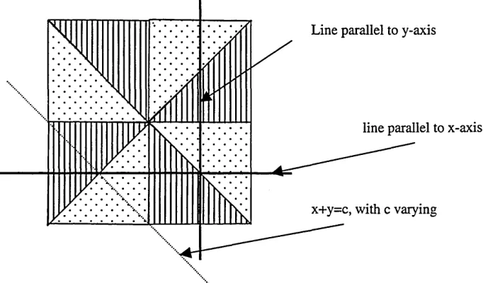
FIGURE B:
Line parallel to y-axis
line parallel to x-axis
x+y=c, with c varying
Figure B above, shows the construction described in Figure A after adding three lines.
We define here:
f (x)g(y) + a if (x, y) is the area shown by dots h(x, y) = - f (x)g(y) - a if (x, y) is the area shown by lines
f (x)g(y) if (x, y) is elsewhere.
It can be seen from the symmetry in the picture in Figure B above, that the deviations ( a ) from the
density values f(x)g(y) corresponding to (X,Y) on the lines shown cancel out. Hence, the marginal
densities of X*,Y* and X*+Y* are the same as those of X, Y and X +Y respectively.
If the bivariate vector (X*,Y*) is taken to be a random vector with density h(x,y)
and the bivariate vector (X,Y) is taken to be a random vector with density f(x)g(y)
as described above, then it follows from all the information above that:
a) X* is distributed as X,
b) Y* is distributed as Y
c) X*+Y* is distributed as X+Y.
Since X*, Y* and X*+Y* have the same distribution as X, Y and X+Y respectively, the corresponding
moments are also the same. We will now consider only the second moments.
If X and Y have the distribution such that E(X2) < °° and E(Y2) < ®°, then
E((X* + Y*))2 = E(X*2)+2E(X*Y*)+E(Y*2) [2a]
E((X+Y)2) = E(X2) + 2E(XY) + E(Y2) [2b]
and E(X*r) = E(Xr), [3a]
From [2a], [2b], [3a] and [3b], it follows that
E(XY) = E(X*Y*)
Since
cov(X,Y) = E(XY) - E(X)E(Y)
= E(X*Y*) - E(X*) E(Y*) = cov(X*,Y*) [4]
and X and Y are independent implying Cov(X,Y)=0, the covariance between X* and Y* equals zero and
X* and Y* are therefore uncorrelated. ,
However, from the construction, it follows that the joint density of X* and Y* does not correspond to
that of independent R.V.’s , implying that they are dependent R.V’s. This is because the marginal
densities of X* and Y* are f(x) and g(y) respectively and there are some areas in Figure A where h(x,y)
* f(x)g(y).
By taking f(x) and g(y) to be normal, we can produce a bivariate distribution for which the random
variables are uncorrelated but dependent. This also implies that even though the marginals here are
normal, the bivariate distribution is not normal. For bivariate normal, uncorrelatedness implies
independence. Since we have in our case R.V is that are uncorrelated but dependent, it follows that their
joint distribution is not bivariate normal.
If we take (Xi,...Xp) with (X!,X2) distributed as (X*,Y*) and (X2,...XP) as normal and independent of
(Xi,X2), then we have a p-dimensional non normal random vector with normal marginals having zero
correlations.
If we are not looking for the new random variables that are not uncorrelated, we get a slightly simpler
construction of a bivariate distribution that is not normal, but has normal marginals; for an alternative
construction of this, see below:
Consider the situation of independent random variables X and Y having probability density functions:
f(x), x 8 (-00,00) and g(y), y 8 (-00,00) respectively.
Here the marginal densities are assumed to satisfy the conditions as before in [1].
Next consider two dependent random variables X* and Y* with the bivariate joint density function
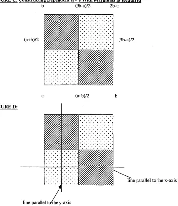
FIGURE C; Constructing Dependent RV’s With Marginals as Required
b (3b-a)/2 2b-a
(a+b)/2 (3b-a)/2
(a+b)/2 b
FIGURED:
line parallel tc/the y-axis
line parallel to the x-axis
Define now h(x,y) such that:
f (x)g(y) + a if (x, y) is in the area shown by dots h(x, y) = • f (x)g(y) - a if (x, y) is in the area shown by lines
f(x)g(y) elsewhere.
We can now see that the marginal distributions of X* and Y* have densities f(x) and g(y) respectively.
If we take f(x) and g(y) to be normal, then it follows that h is the density of a bivariate non-normal
distribution with normal marginals. Also, now (X!,X2,...X P) can be taken as a vector as defined before,
but, with (X*,Y*) as in the present construction. Incidentally, the vector obtained from the previous
construction has Xj’s to be uncorrelated and marginally normal, and in the present construction we have
Xi’s to be just normal.
Note: following the insertion of the lines in Figure D the deviations from the densities relative to X and
Y cancel out as was shown in the previous example.
0973
From the above construction, it is clear that even when we get the respective samples at the various time
points to be from a normal distribution, it does not follow collectively that the normal distribution
assumption usually taken for “Repeated Measures Data Analysis” is met. A way of testing for
multivariate normality would be the recommendation of some approximate techniques.
There is a characterisation of the multivariate normal distribution that a vector (Xi,...Xp) is multivariate
normal if and only if every linear combination of X^.-.Xp are univariate normal [See Theorem 2.6.2 in
Anderson (1958)l3aI]. Since any multivariate normal distribution is determined by the corresponding
moments (i.e. by E(X!k l Xp kp) with k l kp as non negative integers) it is possible to have a
slightly improved version of the result just stated. The improved version is that a vector (Xi,...Xp) is
multivariate normal if and only if m f1Xi+ + m^Xp is univariate normal for each positive integer
m,, i=l,2....P.
This is so especially because the moments are determined by E{exp(Zmi’Xj)}.
Following this, one could suggest an appropriate technique to test normality as follows:
Choose a sufficiently large number N and test univariate normality of m ^ X ^ m^Xp for integers
m j,.. ..mp =1,2, N. If we have positive conclusions for most of the linear combinations, then it is
reasonable to expect (X!,...XP) to be approximately normal.
To test for multivariate normality, one could also devise alternative techniques.
If X i,.. .,Xn is a reasonably large sample from a population, then, provided n > 3 and E|Xr| < °o, we have
that E (XXj/n|(X ! -XXj/n))=constant. [5]
If and only if X /s are normal [see Kagan, Linnik and Rao1341 for the result by Ramachandran and Rao].
The result is also valid in the case when Xr's are vectors, and hence one could use this property to test
for MVN. The test could be devised as follows:
Divide the sample on the p-component vector into smaller samples of equal sizes. Denote XX/n and
Xi - SX /n corresponding to these smaller samples (of sizes > 3) by Uh and U2i respectively. Hence, the
MV normality of Xi, ...X n can be seen to be equivalent to:
E(Ui j|U2i)=constant.
Thus, the problem reduces to that of testing a linear regression. To solve the problem, one could take the
Incidentally, to go from the Ramchandran and Rao (R-R) characterization of the normal distribution in
the univariate case to that for the M.V. case, we can use the characterization given in Theorem 2.6.2 of
AndersonI3a] concerning M.V. normality referred to earlier.
Test in this case only the equations that the conditional expectations of the linear combinations of the
components of Uu with coefficients mf1, given linear combinations of the components of U2i with
coefficients nf1 (where m; and nj are positive integers).
An adhoc approach for analysing the Repeated Measures data is to assume that different units are
independent and that within each treatment group have an identical distribution. With appropriate
changes to the data sets, one could apply the asymptotic theory relative to parametric tests such as
Hotelling’s T2, Mahalanobis D2 or likelihood ratio tests to test hypothesis relative to mean vectors or
appropriate non-parametric tests for the hypothesies that various treatment groups have the same
distribution. The tests applied are obviously more robust, when n is large.
Suppose the sample sizes nj and n2 are large and the Hotelling T2 is given by:
T2 = _2!£2_(xffl -x<2>)'S-'(x® -x<2>)
i>! + n 2
(with obvious notational alterations) as mentioned on page 109 in AndersonI3a]. Then even when the
two populations are not normal, under the hypothesis that the mean vectors of the two populations are
equal, we have the distribution of T2 to be approximately the same as that of Y' I Y where Y ~ N (0,
2 ). Here the Central Limit Theorem (CL) is being assumed together with the assumption of the
populations having the same covariance matrix.
This follows because asymptotically, S = 2, and under H0,
JH
52-(xW _*»))
n i + n 2
is distributed as Y, where Y is as defined here.
From a well known result on quadratic forms it follows that the distribution of Y' 2 Y is %2 with p df.
(Theorem 3.3.3 on p54 of AndersonI3a]). Thus even when the two populations are not assumed to be
normal, the null distribution of T2 becomes a approximately %p2. Incidentally, Hotelling’s T2 is a
constant multiple of Mahalanobi’s D2, which is given by:
For a normal model under H0,
ni + n2 - p - l ^
p(n1+ n 2- 2 )
T ~ F(p,n, + n2 - p - 1 ) .
Indeed in view of the C.L Theorem, it follows that the tests used are asymptotically the same as those
relative to the normal distributions as long as p (the number of components of the vector) is small
compared to ni and n2. or more generally ni + n2. (Note that T2, that is a constant multiple of D2, has its
asymptotic null distributions to be xp2). This remark also applies to the likelihood ratio test or non-
parametric tests for testing that the mean vector relative to the treatment groups are the same as long as p
and the number of groups is not large compared to sample sizes for the groups involved.
In particular, in the case of the vector of 6 components of summary statistics, we can reasonably assume
p (i.e. 6) is small compared to the nj,n2=24 and use T2 or D2 as an approximate test statistic, giving
approximately a Chi-squared test.
Incidentally, if the whole vector is normal, then the components of the vector are normal, though the
converse of this result as shown by our constructions is not valid.
In our analysis, if we find that the normality assumption is not met at some time points then it follows
that the multivariate normality assumption for the data may not be reasonable. One could then look for
ways to make asymptotic (more robust) tests applicable to our data.
The idea is then to reduce the number of repeated measures to a much smaller number so as to satisfy the
condition that the number of individuals is considerably larger than the number of repeated measures,
making asymptotic tests applicable. Under this situation there is no loss of generality in assuming that
2.2 Methods of Analysis
2.2.1: Plotting the Data.
An initial approach in conducting any type of analysis is to carry out some kind of exploratory data
analysis (E.D.A.). We can begin by graphically displaying the data at each time point as follows:
1. Individual profile plots can be displayed together on one plot.
This type of plot can often become very clustered especially if there are too many individuals in the
study. The following two graphs eliminate this issue.
2. Box plots show distribution of the data at each time point.
3. The group means at each time point with standard errors can be displayed together on one plot.
4. The summary statistics such as mean, median, minimum and maximum at each time point can also
be displayed over time.
All plots above display the individual repeated measurements of data separately.
Data can also be summarised for all time points together by following the approach of the ‘Response
Features Analysis’ mentioned in 2.2.2. Here each individual will have a set of single variables that each
represents all the data as a whole (e.g. mean, median, minimum etc.). This information can then be
summarised grap