Joint WGCM/WGSIP Workshop on Decadal Predictability, La Jolla, CA, USA, 4 6 October 2000

(1)

WORLD CLIMATE RESEARCH PROGRAMME

JSC/CLIVAR Workshop on Decadal Predictability

Scripps Institution of Oceanography

La Jolla, CA, USA

October 4-6, 2000

March 2001

WCRP Informal Report No 1/2001

ICPO No. 39

INTERNATIONAL

INTERGOVERNMENTAL

WORLD

COUNCIL FOR

OCEANOGRAPHIC

METEOROLOGICAL

(2)

CLIVAR is a component of the World Climate Research Programme (WCRP), which was

es-tablished by WMO and ICSU, and is carried out in association with IOC and SCOR. The

scien-tific planning and development of CLIVAR is under the guidance of the JSC Scienscien-tific Steering

Group for CLIVAR assisted by the CLIVAR International Project Office. The Joint Scientific

Committee (JSC) is the main body of WMO-ICSU-IOC formulating overall WCRP scientific

concepts.

Bibliographic Citation

(3)

TABLE OF CONTENTS

Executive Summary

5

Appendix 1: List of Participants

7

(4)

(5)

Workshop on Decadal Climate Predictability

Executive Summary

Scripps Institution of Oceanography, La Jolla, CA, USA, 4-6 October 2000

George Boer

Canadian Centre f. Climate Modelling & Analysis, University of Victoria Victoria, Canada

[email protected]

Mojib Latif, Max-Planck-Institute for Meteorology, Hamburg, Germany

Roger Newson, Joint Planning Staff for WCRP, WMO, Geneva, Switzerland

The joint WGCM/WGSIP Workshop on Decadal Climate Predictability took place at the Scripps Institution of Oceanography, La Jolla, CA, USA, from 4-6 October 2000. There were over 30 participants from 18 different scientific institutions, groups and organizations. The ob-jective of the workshop was to form an overall sense of the "state of the art" in decadal predictability. Since this area of study is in its infancy, the intent was a true "workshop" which would explore observed and simulated decadal variability, decadal predictability, and such practical attempts to produce decadal forecasts as were available. The Workshop was organ-ized into a series of presentations in these broad areas followed, on the final morning, by three break-out working groups. The groups summarised the status of observations and observed variability, simulations and simulated variability, and prediction/predictability and made rec-ommendations and suggestions.

Most presentations on observations and simulations focused on interdecadal variability in the Pacific and North Atlantic. Several talks highlighted the multi-decadal variability in the Atlan-tic Ocean. This type of variability has typical time scales of 60-80 years, and it can be described from direct temperature observations and from indirect data for the last millennium. The mul-ti-decadal variability involves an interhemispheric dipole in the Atlantic sea surface temperature, and there is some evidence that it may be predictable several years in advance, based on a perfect-model predictability study made with a coupled ocean-atmosphere general circulation model. Other regions of relatively high "potential" decadal predictability, identified in the control runs of 11 coupled models in the CMIP1 database, are the North Pacific, the trop-ical Pacific and the Southern Ocean. Decadal predictability of surface temperature over land appears to be very modest in these results.

In sum, the workshop considered long time-scale phenomena in the coupled system and the evidence for decadal predictability. There was some indication of predictability, mainly at higher latitudes and associated with long timescales in the ocean, obtained from prognostic perfect model and diagnostic potential predictability studies. The utility and practical achieve-ment of decadal forecasts, nevertheless remains an open question which requires directed attention and active research.

Observations and simulations of decadal variability

(6)

The understanding of the North Pacific Oscillation (or Interdecadal Pacific Oscillation), is also comparatively rudimentary, although there has recently been progress in modelling decadal changes in the North Pacific. In the tropical Pacific, coupling to mid-latitudes does not appear to explain much of the variance (temperature/salinity anomalies may be the key, but these anomalies are small). The role of the Southern Hemisphere oceans, if any, is unknown. Decadal variability could also not be clearly separated from global warming which might itself be re-sponsible for some decadal variability. How global warming might interact with "natural" decadal variability is not yet clear.

As a basis for further progress, much longer time series of data and model runs were seen as essential (i.e. from reanalyses, paleoclimatic data, and extended coupled model integrations). The requirement was also expressed for a multi-decadal ocean and/or coupled ocean/atmos-phere reanalysis for hypothesis testing, for initialising simulations and decadal forecasts.

Predictability and prediction

Some predictability at decadal timescales of the ocean circulation at higher latitudes (particu-larly the thermohaline circulation) was inferred from potential predictability studies and perfect model experiments. Associated variations over land might be predictable also, but only explain a small fraction of the total variance. In the tropical Pacific, some weak evidence of dec-adal predictability was noted. The question of how decdec-adal and interannual variability interact is unanswered. There are large areas where there is yet no firm understanding, namely those concerning the tropical Atlantic dipole, the Interdecadal Pacific Oscillation, and the North At-lantic and the predictability of the North AtAt-lantic Oscillation.

There was some consensus that the thermohaline circulation may be predictable at decadal time scales provided that initial oceanic conditions could be satisfactorily specified. However, the impact of the North Atlantic Oscillation on the export of freshwater from the Arctic re-mained to be clarified. Improved simulations of overflows and deep (ocean) convection which affect temperature/salinity locally were also needed. The interaction between ENSO variabil-ity on decadal timescales and the thermohaline circulation was not well understood. A pioneering attempt at practical decadal forecasting (by the Hadley Centre) is underway but has achieved only modest results to date.

Future directions

It was considered that a vital step in making progress from the current rather elementary po-sition was work on understanding the mechanisms that might underlie predictability (including the study of particular modes). The understanding of the dynamics involved in these mechanisms is limited. Time-scale interactions (e.g. the Interdecadal Pacific Oscillation with ENSO) also needs study.

(7)

Appendix 1: List of participants

Mathew Barlow

IRI International Research Institute

Lamont-Doherty Geological Observatory of Columbia University Route 9W

Palisades, NY 10964 U. S. A.

email: [email protected]

George J. Boer

Canadian Centre for Climate Modelling and Analysis Atmospheric Environment Service

University of Victoria P.O. Box 1700

Victoria, B.C. V8W 2Y2 Canada

Li Chongyin

LASG, Institute of Atmospheric Physics Chinese Academy of Sciences

P.O.Box 2718 Beijing 10080 China

Kim Cobb

University of California

Scripps Institution of Oceanography 9500 Gilman Drive

La Jolla, CA 92093-0236 U.S.A.

Arnaud Czaja

Massachusetts Institute of Technology

Department of Earth, Atmospheric, and Planetary Sciences 77 Massachusetts Avenue

Cambridge, MA 02139-4307 U.S.A.

Gidon Eshel

University of Chicago

Dept. of Geophysical Sciences Ellis Avenue

Chicago, IL 60637 U. S. A.

(8)

Chris Folland

Meteorological Office, Hadley Centre for Climate Prediction and Research London Road

Bracknell, Berkshire RG12 2SY U.K.

Stephen Griffies Princeton University

Geophysical Fluid Laboratory Route 1, Forrestal Campus Princeton, New Jersey 08542 U.S.A.

Mojib Latif

Max-Planck-Institut für Meteorologie Bundesstraße 55

20146 Hamburg Germany

Carine Laurent

Laboratoire de Météorologie Dynamique du CNRS UPMC, Tour 25-15, 5e etage, Boite 99

4, place Jussieu

F-75252 Paris, Cedex 05 France

Peter Lemke Universität Kiel

Institut für Meereskunde Düsternbrooker Weg 20 24105 Kiel

Germany

Michael E. Mann University of Virginia

Department of Environmental Sciences Clark Hall

Charlottesville, VA 22903 U.S.A.

Bryant J. McAvaney

Bureau of Meteorology Research Centre G.P.O. Box 1289 K

Melbourne, Victoria 3001 Australia

(9)

Gerald A. Meehl

National Center for Atmospheric Research Climate&Global Change Division

P.O. Box 3000

Boulder, CO. 80307-3000 U.S.A.

Vikram M. Mehta

NASA/NASA-Univ. of Maryland Joint Center for Earth System Science Department of Meteorology

College Park, Maryland 20742 U.S.A.

Arthur J. Miller

University of California, San Diego Scripps Institution of Oceanography 9500 Gilman Drive

La Jolla, CA 92093-0224 U.S.A.

Roger Newson

World Meteorological Organization WCRP

C.P. 2300

CH-1211 Geneva 2 Switzerland

David Pierce

Scripps Institution of Oceanography University of California, San Diego 0224 9500 Gilman Dr.

La Jolla, CA 92093-0224 U. S. A.

Scott B. Power

Bureau of Meteorology Research Centre G.P.O. Box 1289 K

Melbourne, Victoria 3001 Australia

Mark J. Rodwell

Hadley Center for Climate Prediction and Research Meteorological Office

London Road

Bracknell, Berkshire, RG12 2SY U.K.

(10)

R.A. Schiffer

NASA Headquarters, Code Y 300 E Street, SW

Washington, DC 20456 U.S.A.

Niklas Schneider

Scripps Institution of Oceanography University of California, San Diego 0224 9500 Gilman Dr.

La Jolla, CA 92093-0224 U. S. A.

email: [email protected] oder [email protected]

Neville Smith

Bureau of Meteorology Research Centre P.O. Box 1289 K

Melbourne, Vic. 3001 Australia

email: [email protected] oder

Ronald J. Stouffer Princeton University

Geophysical Fluid Laboratory/NOAA Room 232

P.O. Box 308

Princeton, N.J. 08542 U.S.A.

Geoffrey K. Vallis Princeton University AOS/GFDL

Princeton, NJ 08544 USA

Masahiro Watanabe University of Tokyo

Center for Climate System Research (CCSR) 4-6-1 Komaba, Meguro-ku

Tokyo, 153-8904 Japan

Tamaki Yasuda

The Meteorological Research Institute Climate Research Department

1-1, Nagamine, Tsukuba Ibaraki 305-0052

Japan

(11)

Appendix 2: Extended Abstracts

Characteristic Spatial and Temporal Structures of Pacific Sea

Surface Temperature

Mathew Barlow

IRI at LDEO, Columbia University, Palisades, NY, USA [email protected]

1. Spatial patterns

The Pacific appears to have characteristic spatial patterns that occasionally show a strong in-fluence in sea surface temperature (SST) anomalies for several years at a time. A well known example is the spatial pattern associated with the climate „transition“ of 1976/77 (Fig. 1a), fre-quently identified as a realization of the „Pacific Decadal Oscillation“ (PDO). The period from 1962 to 1966 (a time of severe drought in the northeastern U.S.) was also characterized by a sta-ble pattern, but local to the North Pacific (Fig. 1b). Low frequency variability of the cold tongue region, with some similarity to the El Niño- Southern Oscillation (ENSO), has also been noted (Fig. 1c). In addition to the eastern equatorial centre of ENSO, two additional areas appear to be centres of action (noted by asterisks in the panels of Fig. 1): the central North Pacific and the subtropical eastern Pacific. An examination of the standard deviation of monthly SSTs (Fig. 1d) shows that these two regions are local maxima of variance (and of SST gradient, not shown). Rotated principal component analysis (RPCA) of monthly SSTs yields the basin-wide "PDO" pattern as the second mode (Fig. 1e), behind ENSO, and the North Pacific pattern as the third mode (Fig. 1f). Aside from some high frequency noise, the RPCA time series are virtually iden-tical to the raw time series at the respective centres of action. The regressions to these unprocessed time series are shown in Figs. 1g and 1h.

In summary, the two patterns appear to be robust and of consequence, as they 1. occasionally dominate the SST anomalies for multi-year periods, 2. are the 2nd and 3rd leading modes of RPC analysis, 3. may be regressed directly from the raw data, and 4. are physically related to the climatological distribution of variance.

2. Contribution to patterns from different frequencies

Although the multi-year averages demonstrate a strong low frequency component to these modes, the details of spatial pattern and time evolution have varied considerably between studies. Here, the RPCA time series are used to analyse the time evolution; using the raw time series from the respective centres of action yields nearly identical results. The global relation-ship for the PDO-type pattern (RPC 2) is shown in Fig. 2a, with the contributions from 2mo-1yr periodicities shown in Fig. 2b, from 8-12yr in Fig. 2c, and 15-25yr in Fig. 2d. The same fre-quency breakdown is shown for the North Pacific pattern (RPC 3) in Figs. 2e-h.

For both modes, the high (sub-annual) and low (decadal) frequency parts of the pattern look quite similar in the North Pacific, while differing greatly throughout the rest of the domain.

3. Power spectrum of the PDO

(12)

4. Time evolution of 15-25yr band

(13)

(14)

[image:14.595.76.508.55.740.2]

FIGURE 3: POWER SPECTRUM OF PDO

FIGURE 4: TIME EVOLUTION AT ~22YR

a)

_{PDO (RPC 2) WAVELET SPECTRUM}

b)

_{PDO (125W,20N)}

a) 15-25yr PDO (solid and NP (dashed), 1900-1991

c)

b) Ω Cycle of 15-25 yr PDO NP Evolution (1945-1993 data)

2mo 4mo 8mo 1.3yr 2.6yr

5.3yr

10.6yr 21.3yr

~6 8mo

~11yr

~22yr

2mo 4mo 8mo 1.3yr 2.6yr

5.3yr

10.6yr 21.3yr

~6 8mo

~11yr

~22yr

95%, AR1

[image:14.595.79.490.98.448.2]

(15)

Diagnostic and prognostic decadal predictability

George J. Boer

Canadian Centre f. Climate Modelling & Analysis, University of Victoria Victoria, Canada

[email protected]

Introduction

Predictability is an attribute of a physical system which indicates the rate at which two initially close states separate with time. This rate limits attainable forecast skill in the presence of error. The prognostic “perfect model” approach estimates the decadal predictability of the climate system by calculating the rate of separation of a set of coupled model simulations. The diag-nostic “potential predictability” approach is rather different. The control simulations of coupled models are analyzed for evidence that the long times-cale variability they exhibit rep-resents a “signal” which is assumed to be predictable given enough information.

Perfect model predictability

The “perfect model” calculation is based on three independent simulations with the CCCma coupled GCM (Flato et al., 2000, Boer et al., 2000a, b, c). The simulations are initialized with the same three-dimensional oceanic state but with independent 1 January atmospheric states. The analysis is confined to surface air temperature (SAT) as the primary climatological variable. The “rate of separation” of solutions is obtained from the average squared difference

between all pairs (i, j) of simulations. The scaled quantity ,

where σ2 is the variance obtained from the control run, gives a suitable measure of the “pre-dictability” p. For presentation purposes, the cumulative scaled predictability

is used to average over the forecast range. The top panel of the accompanying Figure displays the geographical distribution of cumulative predictability for annual mean SAT at year 10. Val-ues for which > 0.4 are shaded. There is an indication of predictability for the southern ocean and, to a somewhat lesser extent, the northern oceans. Patchy values are seen also for the trop-ical Atlantic and Pacific.

Potential predictability

Potential predictability is a measure of the variability of the system which attempts to quantify the fraction of long timescale variability that may be distinguished from the natural variability noise. This “signal”, if it exists and is of appreciable magnitude, is deemed to arise from phys-ical processes operating in the system which are, at lease potentially, predictable. The statistical approach generally follows Rowell (1998), and Rowell and Zwiers (1999) and as-sumes SAT variation is of the form T_αβ = µ+ s_α+ε_αβ with µ the climate mean, s_α the slow timescale “signal” component of the variability, and ε_αβ the remaining unpredictable climate noise. The ratio ρ = σ2/(σs2+σe2) gives the fraction of the total variance associated with the

“po-tentially predictable” component. The value is tested against the null hypothesis that ρ = σ_s2=0.

d2( )τ = (y_i( )τ –y_j( ) )τ 2

f( )τ = (d2⁄(2σ2))= (1–p( )τ )

p˜ 1–˜f 1 ---_τ1 f( )τ' dτ' 0

τ

∫

⋅

 

 

 

–

= =

p

(16)

The result is shown in the bottom panel of the Figure. The result does not depend on a single model or simulation but is an ensemble estimate of the potential predictability of the coupled system based on the control simulations of eleven models participating in the Coupled Model Intercomparison Project (CMIP is described briefly in Meehl et al., 1997). The high latitude oceans are the dominant regions exhibiting potential predictability although there is some in-dication also in the tropical Pacific.

Discussion

The decadal predictability of the coupled atmosphere/ocean/ice system is examined using both prognostic “perfect model” and diagnostic “potential predictability” approaches. Both approaches give some evidence of long timescale predictability at high latitudes over oceans and, to a lesser degree, in the tropical Atlantic and Pacific. Decadal predictability over land and sea-ice is generally low. Both predictability approaches have their weak-nesses; the potential predictability approach does not directly denote actual predictability and the prefect model approach may suffer from model imperfections and the smallness of the ensemble of simula-tions. The results direct attention to the high latitude oceans as the apparent seat of the dominant mechanisms determining decadal predictability.

(17)

References

Boer, G.J., G. Flato, M.C. Reader, and D. Ramsden, 2000a: A transient climate change simulation with greenhouse gas and aerosol forcing: experimental design and comparison with the instrumental record for the 20th century. Climate Dynamics, 16, 405-425.

Boer, G.J., G. Flato, and D. Ramsden, 2000b: A transient climate change simulation with greenhouse gas and aerosol forcing: projected climate for the 21th century. Climate Dynamics, 16, 427-450.

Boer, G.J., 2000c: A study of atmosphere-ocean predictability on long timescales. Climate Dynamics, 16, 469-477.

Flato, G.M., G.J. Boer, W. Lee, N. McFarlane, D. Ramsden, and A.Weaver, 2000: The CCCma global coupled model and its climate. Climate Dynamics, 16, 451-467.

Meehl, G.A., G.J. Boer, C. Covey, M. Latif, and R.J. Stouffer, 1997: Intercomparison makes for a better climate model. EOS, 78, 445-451.

Rowell, D., 1998: Assessing potential seasonal predictability with an ensemble of multidecadal GCM simulations. J. Climate, 11, 109-120.

Rowell, D., and F. Zwiers, 1999: The global distribution of sources of atmospheric decadal variability and mechanisms over the tropical Pacific and southern North America. Climate Dynamics, 15, 751-772.

10 25 50 75

(18)

Atmospheric Circulation Anomalies and Inter-decadal Climate

Variation in China

Li Chongyin and Mu Mingquan

LASG, Institute of Atmospheric Physics, CAS, Beijing, China [email protected]

1. Inter-decadal Climate Variation in China

The climate jump in the 1960’s has been indicated in some studies and it was only one climate jump event represented completely by observational data until now (Yamamoti, 1986; Yan, et al., 1990; Wang, 1990). In fact, the climate jump in the 1960’s showed clearly the feature of in-terdecadal variation of the climate. For this climate jump, many elements, such as precipitation, temperature and surface pressure, all had obvious signal. The sudden variations were all in the period from 1962 to 1967, and a precedent large-scale jump signal occurred at 500 mb height over the mid-latitude Atlantic region in the late of the 1950’s (Yan, 1992). In or-der to unor-derstand the climate jump in 1960’s, two examples in China can be shown as follows: one is shown by using temporal variation of the summer (June-August) precipitation anomaly (%) in Huabei region. It is very clear that there were mainly positive precipitation anomalies before 1964 but mainly negative precipitation anomalies from and after 1964. An obvious cli-mate jump occurred in 1964 in Huabei region. The averaged summer precipitation changed suddenly from the stage more than normal to the stage less than normal. The second is shown in temporal variation of the surface air temperature anomaly in winter (December-February) in Sichuan province. We can find that the winter temperature in Sichuan was changed into the cold period since 1962 because there were mainly negative temperature anomalies after 1962. Even though positive anomalies during the shorter time were in existence, it still means an ob-vious climate jump occurred in Sichuan in 1962, and the averaged surface air temperature in winter changed suddenly from warm stage to cold stage. The variation feature of winter tem-perature in Sichuan is similar with that given in the reference by Wang. Obviously, based on above-mentioned analyses and previous research results, it is very evident that a climate jump occurred in the 1960’s and the inter-decadal climate variation in China was demarcated in the 1960’s.

2. Anomalous Patterns Corresponding to Atmospheric Circulation NAO and NPO

(19)

3. Numerical Simulations with GCM

In this section, the simulated climate characteristics in the eastern China will be discussed, in-cluding air temperature and precipitation. Meanwhile, their similarity and difference to the observation will be analysed further. The interdecadal oscillations, including 10~20 and more than 30 years, are striking in the temporal variation of the seasonal mean air temperature de-parture in the eastern China (20o~40oN, 110o~120oE) and the time period cross-section of its wavelet coefficient. There is well positive correlation of the air temperature anomaly in the eastern China with East Asian trough variation. Strong East Asian trough (negative height de-parture) is corresponding to the low air temperature in the eastern China (negative air temperature), vice versa, the weak trough is accompanied by the high temperature in the east-ern China. The two variables’ association on the inter-decadal time scale is analogous to that on the weather time scale. So, their physical processes are consistent and apparent. In order to be more clearly reflected the characteristics of the climate inter-decadal variation, the variables will be done with the low pass filter so that the variation below the inter-annual time scale (on-ly containing above 7 years oscillation) is ironed out. The features of the inter-decadal variations are considerably apparent not only in the anomaly of East Asian trough and air tem-perature in the eastern China but also in that of the precipitation in North China. It is specially noticed that the climate abrupt change in the 1960s has been found in the past investigations (Yan et al., 1990; Li and Li, 1999). It further exhibits that this abrupt also exists in the simulated results. At the same time, the abrupt change of air temperature is parallel to the variation of the geopotential height at 500 hPa. All of these are consistent with the observation very well (Wang et al., 1998). Above all, the AGCM can well simulate not only the interdecadal variation of climate and atmospheric circulation but also their associated component, the climate abrupt change during the 1960s.

4. Conclusions

The main purpose of the paper is to analyse the inter-decadal change features of the atmos-phere general circulation. Although observational data is not enough but the analyses can clearly show that there is the evident inter-decadal variation exists in the evolution of the gen-eral circulation, mainly including the 10-20 and more than 30 years quasi-periodical variations. It shows clearly not only in the main atmospheric oscillations, but also in some important weather and climate systems. The intensity changes of Western Pacific subtropical high, East Asian and North American trough are in phase or out-of-phase some time as to the 10-20 years quasi-periodical. To the more than 30 years quasi-periodical, they show mainly in phase, and West Pacific subtropical high change goes ahead of 5-7 years.Parallel to the inter-decadal var-iation of atmospheric circulation, climate anomalies in the eastern China, including the abrupt change during the 1960s, are quite well grasped by the simulation of the AGCM too. The nu-merical experiment with GCM is also a useful approach and technique to investigate the inter-decadal variation of atmospheric circulation and global climate.

References

Chongyin, L., and L. Guilong, 1999: Variation of the NAO and NPO associated with climate jump in the 1960s. Chinese Sci. Bull., 44 , 1983-1987.

Shaowu, W., 1990: The variation tendency of temperature in China and the globe during the last one hundred years (in Chinese). Meteorology, 16, 11-15.

Shaowu, W., et al., 1998: Construction of the near 100 years air temperature in China. Quart. J. Appl. Meteor., 9, 392-401.

(20)

Zhongwei, Y., 1992: A primary analysis of the process of the 1960s northern hemispheric summer climatic jump. Chinese J. Atmos. Sci.,16, 111-119.

Yan, Z., J. Ji, and D. Ye, 1990: Northern hemispheric summer climatic jump in the 1960’s, I: Precipitation and temperature. Science in China (B), No.1, 97-103.

Labrador sea convection and the path of the North Atlantic

current in a coupled model

Claire Cooper and Chris Gordon

Hadley Centre, Met. Office, Bracknell, UK [email protected]

Introduction

This paper investigates the existence and causal mechanisms of decadal SST anomalies in the NAC region as simulated in the latest Hadley Centre coupled climate model (HadCM3, Gor-don et al., 2000). It is the detailed modelling and understanding of these mechanisms which may, in the future, enable some degree of predictability of natural climate variability. Dickson et al. (1996) have shown that co-ordinated changes, forced by the North Atlantic Oscillation (NAO), have been occurring in the region over the last fifty years. Sutton and Allen (1997) an-alysed observed wintertime North Atlantic SSTs and calculated lagged correlations over the entire basin with a source region in the vicinity of Cape Hatteras. These indicated that anom-alies originating near Florida in the subtropics appear to propagate along the path of the NAC, taking approximately nine years to cross the basin. This is much slower than the advective speed of the NAC.

Model simulation compared to observations

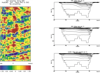
The control integration of HadCM3 has completed over 1000 years and figure 1 shows the NAOI (Hurrell, 1995) from the coupled model for the first 1000 years of the simulation. Choos-ing a period of the control in which NAO variability is similar to that in the ocean observed record we have made a comparison with LSW production. As in the observations the NAOI and LSW production indicators show a clear anti-correlation relationship during this period. Therefore in the model, as in the observations, there is a positive correlation between the NAO and Labrador Sea convection. As shown in figure 2, the model also simulates propagating SST anomalies similar to those found in the observational data by Sutton and Allen.

Labrador Sea Convection Experiments

(21)

[image:21.595.171.423.86.286.2]

Figure 1. NAO index for the first 1000 years of the HadCM3 control experiment, calculated using normalised wintertime (DJF) sea level pressure differences between Lisbon (Portugal) and Stykkisholmur (Iceland), defined and smoothed as Hurrell (1995). Heavy line is the smoothed index.

Figure 2 (left). Model wintertime (DJF) sea surface temperature (oC) anomalies along the mean path of the

model North Atlantic current. ‘X’ marks the region in which the sub-polar and sub-tropical gyres meet (off Newfoundland). No smoothing has been applied.

Figure 3 (right). Potential density (σ₀) cross-section at 50oN. Wintertime mean, year 10 (a) CONV, (b)

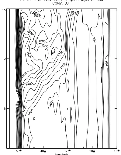
[image:21.595.109.499.357.641.2]

(22)

[image:22.595.81.518.294.564.2]

Figure 3 shows annual mean potential density (σ₀) at year 10 on a cross section at 50oN from the North American coast to the European continent. The increased volume of density class 27.9 to 28.0 in CONV is striking, as is the steepening of the frontal structure at 30oW. There is little change to the structure across the basin in INHIB. This implies that forcing convection has led to a more voluminous water mass (LSW, density 27.9 to 28.0) relative to both the control and the case with inhibited convection. The frontal structure observed at 30oW is associated with the NAC, the steepening of the front being linked with an intensification of the northward component of the current in this location. The development of the 27.9-28.0 water begins on the western side of the basin as a thickening of the layer. The evolution of this feature can be seen in figure 4 a distance-time section of the thickness of the 27.9-28.0 isopycnal layer across 50oN. A thikkening of this layer first appears on the western extreme of the section after ap-proximately four years. This thickening continues and moves eastward until reaching 30oW after a further four years. SST changes at 50oN behave in a similar way to changes in LSW thickness and these changes in SST also propagate eastwards at this latitude. After approxi-mately 3-4 years of convective forcing a large SST anomaly appears to the south of Newfoundland which then propagates north eastwards along the NAC (not shown).

Figure 4 (left): (a) Thickness of isopycnal layer (27.9<σ₀<28.0) at 50oN from CONV. Wintertime means

(DJF).

Figure 5 (right): Cyclic forcing experiment, detrended and filtered (retaining 7-20 years) wintertime SST

anomalies (oC) along the mean path of the modelled North Atlantic Current (taken from HadCM3 control).

X’ marks the region in which the sub-polar and sub-tropical gyres meet (off Newfoundland).

[image:22.595.80.279.301.555.2]

(23)

the first half of thecycle followed by convection enhancing conditions for the later part of the cycle. The experiment was run for 42 years allowing the completion of three cycles. To extract the decadal signal the data have been filtered, removing signals of less than 7 years and greater than 20 years. Figure 5 shows the filtered SST anomalies from this cyclic forcing simulation along the mean pathway of the control NAC. A pulsating 14-year SST anomaly signal is very evident at the point where the NAC turns north. The anomaly then propagates to the east with decreasing amplitude. This experiment gives a clear illustration of how decadal variations of deep convection in the Labrador Sea can lead to corresponding SST variations propagating along the path of the NAC.

References

Curry, R., M.S. McCartney and T.M. Joyce, 1998: Oceanic transport of subpolar climate signals to mid depth subtropical waters. Nature, 391, 575-577.

Dickson, R.R., J.R.N. Lazier, J. Meincke, P. Rhines and J. Swift, 1996: Long-term co-ordinated changes in the convective activity of the North Atlantic. Prog. Oceanogr., 38, 241-295. Gordon, C., C. Cooper, C.A. Senior, H.T. Banks, J.M. Gregory, T.C. Johns, J.F.B. Mitchell and

R.A. Wood, 2000: The simulation of SST, sea ice extents and ocean heat transports in a

version of the Hadley Centre coupled model without flux adjustments. Climate

Dynamics, 16, 147-168.

Hurrell, J.W., 1995: Decadal trends in the North Atlantic Oscillation: Regional temperatures and precipitation. Science, 269, 676-679.

(24)

Observations of Atmosphere - Ocean coupling

in the North Atlantic

Arnaud Czaja and John Marshall

Department of Earth, Atmospheric, and Planetary Sciences, Massachussets Institute of Technology, Cambridge, MA, USA [email protected]

1. Introduction

Deser and Blackmon (1993), on the basis of an Empirical Orthogonal Function (EOF) analysis of surface climate variable in winter (1900-89), have isolated a large - scale SST pattern whose power spectrum shows a broad band peak near the decadal period. The SST pattern shows op-posite sign SST anomaly, roughly north and south of the mean position of the separated Gulf Stream, and also extends to the eastern subtropics, such as to form a tripolar SST pattern. The associated surface atmospheric circulation is reminiscent of the North Atlantic Oscillation (hereafter the NAO), and similarly exhibits enhanced power at the decadal period. Although Deser and Blackmon (1993) have suggested that the decadal timescale may be due to changes in the thermohaline oceanic circulation, there is not yet a consensus on the mechanisms gov-erning the low frequency evolution of the SST ’tripole’. Grötzner et al. (1998) have argued that it may reflect an interaction between the NAO and the wind driven ocean circulation, as they found such interactions in a long integration of a coupled Atmosphere - Ocean model. The lack of long observational records of subsurface oceanic data is clearly a limiting factor to evaluate the role of the ocean circulation in the decadal variability seen at the surface. Also, lots of stud-ies lack a theoretical framework to use as a guide in the analysis of the available observations. The interpretation of the results is even made more difficult by the use of complex and elabo-rate statistical techniques (EOFs, Principal Oscillation Patterns, multivariate frequency domain methods, etc ...).

Here, to explore evidence and possible mechanisms of atmosphere-ocean coupling, we intro-duce and study a simple SST index ∆Τ from a long observational record (1856 - 1998); it measures the strength of the dipole of SST that straddles the Gulf Stream and was chosen be-cause (i) it is a measure of low level baroclinicity to which cyclogenesis at the beginning of the Atlantic storm-track may be sensitive (ii) it may be sensitive to anomalies in ocean heat trans-port associated with both wind driven gyres and thermohaline circulation. Pronounced decadal signals in ∆T are found which covary with the strength of sea level pressure (hereafter SLP) anomalies over the Greenland - Iceland Low and subtropical High regions. Using the sim-ple cousim-pled model developed in Marshall et al. (2001), we interpret features of the power spectrum of observed SST and SLP as the signature of coupled interactions between the atmos-pheric circulation and an anomalous wind driven ocean gyre.

2. A cross Gulf Stream SST index

(25)

tripole has been generated (Fig. 1, bottom middle panel), the tripole reappears 6 yrs later, but with opposite sign (Fig. 1, bottom right panel).

Figure 1: (Upper panel): timeseries of the

SST index ∆T = T_N -T_S. (bottom panel).

Composite maps for SST (in K). The black lines indicate the 95% confidence level for the SST composite maps. See text for details.

Based on a similar composite analysis with the long observational record of SLP by Kaplan etal.(1999), we found that the atmospheric conditions

associ-ated simultaneously with ∆T are

reminiscent of the NAO (not shown), although slightly shifted southwest-ward. They show opposite sign anomalies over the Greenland - Ice-land Low (hereafter GIL) and subtropical High (hereafter STH) re-gions, such that in yrs when SST are warmer north than south of the Gulf stream (∆T > 0), the surface atmospheric circulation is weakened. We argue in the following that the sign reversal exhibited by the SST tripole after 6 yrs is driven by the delayed adjustment of the wind driven ocean circulation to the NAO surface wind forcing. As shown below, advection can success-fully explain the change of sign of SST anomalies near the separated Gulf stream. It is suggested that the sign reversal of subtropical SST is driven locally by turbulent surface heat flux, reflecting the NAO response to changes in ∆T.

3. A model for the decadal evolution of ∆T

[image:25.595.77.329.102.321.2]

Using the NCEP - NCAR reanalysis, we have computed the equilibrium response of the ocean circulation to the weakening / strengthening of the surface winds associated with ∆T anoma-lies, according to linear at bottom Sverdrup dynamics (Fig. 2). The geostrophic streamfunction consists, following yrs where the winds blow stronger over the ocean (i.e., yrs when ∆T < 0), in an anticyclonic circulation connecting the two boxes used to define ∆T. Following Marshall et al. (2001), we speculate that the path of the separated Gulf stream is anomalously poleward when the gyre circulates anticyclonically, so that the northern box is anomalously warmed and the southern box anomalously cooled. Thus, the wind driven circulation acts to change the sign of an initial ∆T anomaly. Scaling arguments for the relative magnitude of local surface heat flux (latent+sensible) and advective heat flux due to the anomalous gyre suggest that the two are of same order (10 Wm-2) on decadal time scales (not shown).

Figure 2: Anomalous geostrophic transport (contoured every Sv) inferred from linear Sverdrup dynamics. The climatological mean position of the zero wind stress curl line, which separates the subpolar and subtropical gyres, is indicated by the thick black line. The two boxes used to

define ∆T are also indicated.

1850 1870 1890 1910 1930 1950 1970 1990

2 1.5 1 0.5 0 0.5 1 1.5 2

TN TS (Feb March Apr)

TIME ( yr )

TN

TS ( K )

HIGH LOW

80oW 60oW 40oW 20oW 0o

0 20 40 60

3 YR LATER

0 20 40 60

6 YR LATER

0 20 40 60

1 0.8 0.6 0.4 0.2 0 0.2 0.4 0.6 0.8 1

SST anomaly (K)

90o

W

72o_W

54o_W

36oW

18oW

(26)

The previous advective mechanism can be easily be added to the canonical model for SST anomalies (Frankignoul and Hasselmann, 1977), in the form of an oceanic heat flux Qo

d∆T /dt = a∆P - λ∆Τ + Qo

where ∆P = GIL - STH denotes the dipolar SLP anomaly associated with ∆T (i.e., the NAO sig-nature in SLP), generating surface turbulent heat exchange with the ocean, as measured by the scaling factor a, and where λ is a damping timescale for ∆T resulting from local air sea interac-tions (about a yr). We consider the following model for Q_o

expressing that, after a delay t_y, the anomalous gyre circulates cyclonically in response to pos-itive ∆P anomalies, and cools ∆T at a rate set by the parameter b (b is of same order as a, as discussed previously). The delay time t_y is controlled by the baroclinic adjustment of the gyre to surface windstress curl changes, and is set to a nominal value of 10 yrs.

Figure 3: Model predictions for ∆P (upper plots)

and ∆T (lower plots), for b = 0 (red), b≠0 but no

feedback of ∆T on ∆P (blue), b≠0 with a small

feedback of ∆T on ∆P (green). The frequency is

expressed in cyle per t_y, i.e., in cycle per 10 yrs.

The power is non dimensional.

One readily sees from (2) that on timescales

> ty, , so that compared to the

hypothetical situation where the ocean cur-rents would not impact SST, the level of the forcing in (1) is reduced from a ∆P (no ocean currents) to (a-b)∆P (ocean circula-tion included). A signature of the role of ocean circulation is thus to decrease the power of ∆T on timescales longer than about 10 yrs, thereby peaking the SST spectrum in the decadal band (Fig. 3, lower plots). When a small impact of ∆T on ∆P is allowed, the peak is even more pronounced and may also be found in ∆P (Fig. 3, upper plots).

4. Comparison with the observations

Figure 4 shows the observed power spectra for ∆T (green), GIL (blue) and STH (red). In good agreement with the previous model (Fig. 3, green curve), the power spectrum of ∆T shows a broad band peak in the decadal band, with no flattening on longer timescales, but instead a continuous decrease of power. The power spectra of GIL and STH are similar up to timescales of about 25 yrs (Fig. 4, blue and red curves respectively). This is consistent with a spectral co-herence analysis, which indicates strong coco-herence and a robust out of phase relationship between GIL and STH up to 25 yrs (not shown), in agreement with the NAO paradigm. On longer timescales, however, the two spectra have different structures and the coherence be-tween them is reduced (not shown). While the STH power spectrum keeps increasing with timescales, that of GIL decreases. The NAO index of Hurrell (1995), the normalized SLP differ-ence between Iceland and Lisbon, has a power spectrum very similar to that of STH (not shown). The decrease of power seen in GIL at timescales > 25 yrs is in agreement with the mod-el predictions when feedback is allowed (Fig. 3, top panmod-el, green curve). We have checked that GIL and ∆T keep coherent on these long timescales (not shown). Thus, although it is a highly simplified view of the dynamics of GIL, our results are consistent with a control of the strength of the Greenland - Icelandic Low by ocean circulation, through its impact on the surface baro-clinicity (as measured by ∆T).

Q₀ (b t⁄ y) ∆P td

t–t_y

( )

t

∫

–

=

10 2 10 1 100 101

10 1

100

101

FREQUENCY (cycle per t_y)

POWER (adim)

no ocean circulation ocean circulation, no feedback ocean circulation and feedback

(27)

Figure 4: Observed power spectra of SLP anomalies near Greenland - Iceland (GIL, blue) and near the subtropical High (STH, red). The power spectrum of the cross Gulf Stream SST

index ∆T is also plotted (green). The frequency is

expressed in cycle per yr and the power in K2/

cpy for ∆T and mb2/cpy for GIL and STH. The

vertical bar indicates the 95% confidence level. Note that the colors chosen here do not refer necessarily to those of Fig. 3.

5. Discussion and comparison with previous studies

Our analysis of the observations is close to that of Deser and Blackmon (1993), although we use simpler techniques and a longer dataset. In agreement with the result of their EOF analysis (their ’dipole mode’), we showed evidence for a pronounced decadal timescale in the variabil-ity of North Atlantic SST. Both their second SST principal component and the ∆T index introduced here show a broad band peak in the 10 -20 yr band, as expected from the similarity between our SST index (SST difference across the separated Gulf Stream) and their 2nd EOF pattern. Nevertheless, the power spectra differ at timescales longer than about 25 yrs: whereas ∆T shows decreasing power with timescales (Fig. 4, green curve), their PC2 shows the opposite (their Fig. 3a). The different data set used (COADS vs Kaplan) may be a possible explanation. However, as the power spectrum of the 1st EOF of North Atlantic SST in winter with the Ka-plan et al. (1997) reanalysis shows a similar power spectrum as that of the second EOF in Deser and Blackmon (1993), with very similar pattern (the tripole), this explanation does not seem valid. Instead, the difference in power spectrum is likely to result from the EOF analysis em-ployed by Deser and Blackmon, which emphasizes large - scale pattern and reflects SST variability outside the Gulf Stream region, whereas our analysis only considers the difference of SST across the Gulf Stream. Independently, we showed that a similar spectral feature is found in SLP anomaly near the Greenland - Iceland Low region (Fig. 4, blue), which keep co-herent with ∆T at these long timescales (not shown). The use of a longer dataset in our study (143 yrs instead of 90 yrs) also certainly allows a better, although still limited, investigation of these long timescales.

More fundamentally, we have proposed a plausible mechanism explaining this decrease of power in ∆T at low frequency. This feature is expected based on linear Sverdrup dynamics, and results primarily, at long timescales, from a partial cancellation of the advective forcing of ∆T anomalies by anomalous ocean currents (the intergyre gyre of Fig. 2), and the local surface forcing of ∆T by the atmosphere. We note that the tendency for Atlantic SST anomaly to be-come of basin extent at interdecadal timescale (Kushnir, 1994) may also be a factor explaining the decrease of power seen in ∆T.

Allowing a small feedback of ∆T on the NAO, Atmosphere - Ocean coupling may peak the spectra of ∆T and SLP near the decadal band, in good agreement with the observed ∆T and GIL spectra. The different structure seen in the latter and that of the NAO or SLP anomaly near the subsidence region (Fig. 4) at low frequency (periods longer than 25 yrs) is intriguing. It is not consistent with our theory which would predict a decrease of power for the whole NAO pat-tern. This may reflect that, in late winter, other factors than ∆T / storm - track interactions control the strength of SLP anomaly over the subsidence region. This requires further study.

10 3 10 2 10 1 100

10 1

100

101

102

FREQUENCY (cycle per yr)

POWER (K

(28)

References

Deser C., and M. L. Blackmon, 1993: Surface climate variations over the North Atlantic Ocean during winter: 1900-1989. J. Climate, 6, 1743-1753.

Frankignoul, C., and K. Hasselmann, 1977: Stochastic climate models, part II: application to sea-surface temperature variability and thermocline variability. Tellus, 29, 289-305. Grötzner, A., M. Latif, and T.P. Barnett, 1998: A decadal climate cycle in the North Atlantic

Ocean as simulated by the ECHO coupled GCM. J. Climate, 11, 831-847.

Hurrell, J., 1995: Decadal trends in the North Atlantic Oscillation: regional temperature and precipitation, Science, 269, 676-679.

Kaplan, A., Y. Kushnir, M. Cane, and B. Blumenthal, 1997: Reduced space optimal analysis for historical datasets: 136 years of Atlantic sea surface temperatures. J. Geophys. Res., 102, 27,835-27,860.

Kaplan, A., Y. Kushnir, and M. Cane, 2000: Reduced space optimal interpolation of historical marine sea level pressure: 1854-1992. J. Climate, 13, 2987-3002.

Kushnir, Y., 1994: Interdecadal variations in North Atlantic sea surface temperature and associated atmospheric conditions. J. Climate, 7, 141-157.

Marshall, J., H. Johnson, and J. Goodman, 2001: A study of the interaction of the North Atlantic Oscillation with the ocean circulation. J. Climate, in press.

North Atlantic Persistence and Decadal Forecasting

Gidon Eshel

Dept. of the Geophysical Sciences, The Univ. of Chicago, Chicago, USA [email protected]

I examine decadal predictability in the North Atlantic. A region near Cape Code and the Gulf of Maine is identified as featuring the highest North Atlantic persistence (Fig. 1 left), with a unique combination of high- amplitude, persistent sea surface temperature anomalies, associ-ated with substantial upper ocean heat content anomalies (Fig. 1 right). A mechanism is advanced, whereby that region's surface ocean is a `window' to deep upper ocean dynamics, with thermal evolution that tracks heatflux divergence by the slowly adjusting subtropical gyre. This is consistent with the subtropical gyre playing a central role in NA climate variabil-ity. The proposed interpretation is supported by broad, high lag correlations between the Bermuda potential vorticity timeseries (representing the subtropical gyre state) and surface anomalies (Fig, 2; the same for SSTA is not shown here). Successive lag correlation patterns re-veal surface oscillations that are not apparent in the raw surface data.

(29)

Figure 1: Left Column: Two measures of `total' persistence. (a) The number of significant lags out of the total number of lags considered. See text for details on the significance test. (b) Sum of squared acf at all lags. Right Column: (a) Root mean square of July-August and February-March SSTA means. (b) The correlations between these 2 means. (c) The product of panels a and b.

90˚W 60˚W 30˚W 0˚

0 ˚ 30 ˚N6 0 ˚N Latitude 30 30 30 40 40 50

N

_sig

a

90˚W 60˚W 30˚W 0˚

Longitude 0 ˚ 30 ˚N6 0 ˚N Latitude 3 3 4 4 4

acf

2

b

Latitude 0.3 0.4 0.5 0.6 0.6

a

SSTA rms (JA , FM)

Latitude 0.3 0.3 0.3 0.4 0.5 0.5 0.5 0.5

b

(JA , FM) Corre--lation Longitude Latitude 0.2 0.2 0.25 0.25 0.3

c

a x b

(30)

Fig. 2: Lagged correlation maps between the PV timeseries and those of SLPA at representative lags.

90˚W 60˚W 30˚W

30 ˚N6 0 ˚N Latitude -0.2 -0.10 0 0.1 0.1 0.2 0.2 0.3 0.4 0.5 0.5

Lagged Correlations Over 1954-1997 of Bermuda PV With

DJFM-Mean SLPA Anomalies Leading Feb Bermuda PV by L Years

L=-9

90˚W 60˚W 30˚W

30 ˚N6 0 ˚N Latitude -0.3 -0.3 -0.2 -0.1 0 0 0.1 0.1 0.2 0.3 0.4

L=-8

90˚W 60˚W 30˚W

Longitude 30 ˚N6 0 ˚N Latitude -0.4 -0.3 -0.2 0 0.1 0.1 0.2 0.2 0.3 0.4 0.5

L= 0

90˚W 60˚W 30˚W

30 ˚N6 0 ˚N -0.4 -0.3 -0.3 -0.2 -0.2 -0.1 -0.1 0 0.1 0.3

L= 5

90˚W 60˚W 30˚W

30 ˚N6 0 ˚N -0.5 -0.4 -0.3 -0.1

-0.1-0.1 0 0.1

L= 6

90˚W 60˚W 30˚W

(31)

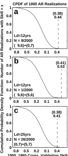
Fig. 3 (above): A schematic of the forecasting method. See text for deatils.

Fig. 4 (right): Cross validation forecasting results for 3 segment combinations against AR(1)-derived, 2000 member population. See text for details.

Dimension 1

Dimension 2

Target State Initial (uncertain)

State State

Later

Schematic 2D Phase Portrait

Flow 0.8 0.5 0.2 0.1 0.4

0 0.2 0.4 0.6 0.8 1

a

( 9,6)+(0,7) N = 9/2000

0.44 (0.38)

Ld=12yrs

CPDF of 1000 AR Realizations

0.8 0.5 0.2 0.1 0.4 0

0.2 0.4 0.6 0.8 1

b

( 9,6)+(5,6) N = 1/2000

0.53 (0.41)

Ld=12yrs

0.8 0.5 0.2 0.1 0.4 0

0.2 0.4 0.6 0.8 1

c

(0,7)+(5,7) N = 26/2000

0.41 (0.38)

Ld=25yrs

Cumulative Probability Density Function: Number of AR Realizations with Skill > x

[image:31.595.354.491.77.389.2]

(32)

Observed variations of climate variability

over the last 100 years

Chris Folland and Robert Allan

Hadley Centre, The Met Office, Bracknell, UK [email protected]

This selective review concentrates on the longer time scales of variability over the last century or more, mainly on large scales. There is some concentration on the Atlantic. Decadal to multi-decadal climate variability over about the last century must be seen against a background of global warming which itself may influence variability, or affect how variability is observed or interpreted. In addition, many of the data used to study climate variability and change were either not designed for the purpose or have suffered from numerous inhomogeneities. Com-pounding this problem are time-varying data gaps, some remaining to this day. Indeed the spatial coverage of some data is now declining. Particularly important are radiosonde data needed for studying the spatial structure of decadal phenomena throughout the full depth of the atmosphere, often within the context of reanalyses. Here a decline in coverage has occurred since the 1980s. New methods are, however being developed to estimate data where gaps are large. These techniques, e.g. the method of reduced space optimum interpolation (Kaplan, 2000), must be viewed with caution. Their correct use requires note to be taken of strong non-stationarities in the data (Hurrell and Trenberth, 1999).

At present there is only limited consensus on the topic of decadal to multidecadal variability, so this brief review can only be preliminary. Useful reviews are given by Enfield and Mestas-Nuñez (1999) and Allan (2000). This note gives a more personal slant. The longest time scale of variability over the last century is the anthropogenic warming of the globe. The globe has warmed (to 1999) by 0.6 ± 0.2oC (95% confidence limits) since the late nineteenth century in two main phases, 1910-1945 and 1976-the present. The spatial pattern of this warming cannot be regarded as fixed, though it may be estimated usefully on specific time scales using EOF meth-ods. Such patterns may be the result of both external forcing (likely to be the largest component when viewed on the global average) and variability internal to the climate system. The latter is especially likely to be important for regional warming trends. Taken over the century, most parts of the world have warmed, though an exception until recently, at least, has been an area south of Greenland. However, nothing reliable can be said about the trends in the Southern Ocean south of 50 oS until the 1980s when there is some evidence of rather muted warming in places. There is also recent evidence of reduced warming of air temperature over the oceans compared to the sea surface in the Indian Ocean and parts of the South Pacific that appeared to commence around 1991. Note that our picture of the magnitude of warming in sea surface temperature (SST) depends on the veracity of large corrections to SST data for their apparent cold biases before 1942.

(33)

Fig. 1: a) Distribution of correlations for the years 1857 to 1996 between local monthly SST anomalies versus the third EOF "Atlantic Multidecadal Mode" b) Temporal realization of the Atlantic Multidecadal Mode computed from temporal amplitude time series and the area-average spatial loadings over the rectangular area in the North Atlantic. In Landsea et al. (1999) - from Enfield and Mestas-Nunez (1999).

An atmospheric pattern that varies on all time scales from days to many decades is the North Atlantic Oscillation (NAO) (Hurrell, 1995) and its close cousin, the Arctic Oscillation (AO) (Thompson and Wallace, 2000, Thompson et al., 2000). The pattern of the AO is one of either relatively high or low pressure across the polar cap and nodes of opposite sign centred near the Azores high and possibly in the mid latitude North Pacific. The NAO exists year round but its pattern varies and it is best developed in winter (but see below). The AO is of larger scale and very often includes the NAO as a component. The main controversy over the AO is wheth-er the weakwheth-er mid latitude Pacific component is real or an artefact of analysis. Othwheth-erwise it is clear that this is a major component of the mid to high latitude Northern Hemisphere atmos-pheric circulation, affecting the stratosphere in the winter, particularly around January to March. Both oscillations have undergone pronounced multidecadal variability with a strong tendency since 1970, and particularly 1988, to move to the positive sign of both modes with rel-atively low pressure over the Arctic.

The NAO is related to a tripole pattern of SST anomalies in the North Atlantic on interannual to quasi-decadal time scales. This pattern has one node in the higher latitudes of the North At-lantic, a node of opposite sign off the east coast of USA stretching across the subtropical Atlantic and a node of the same sign as in the higher latitudes in the tropical North Atlantic. The tripole appears to be driven by the North Atlantic Oscillation on a variety of time scales, and in turn there is evidence that it may force the NAO to some extent (Rodwell et al., 1999).

Thompson and Wallace (2000) show that there is a similar “polar cap” pattern to the AO in the Southern Hemisphere that was in fact first described by Kidson (1988), and called by Thomp-son and Wallace the Antarctic Oscillation (AAO) and by KidThomp-son the High Latitude Mode. This mode has a similar vertical and horizontal structure to the AAO despite the very different

sur-Interhemispheric Thermal Contrast or

(34)

face conditions represented by Antarctica. The history of this mode is poorly known, but atmospheric data are probably good enough to define its behaviour over the last 30 years. Like the AO, the AAO appears to have multidecadal variability and has also gone into a positive mode since the late 1980s.

There appear to be modulations of the interannual El Niño-Southern Oscillation (ENSO) vari-ations on decadal to multidecadal time scales which are particularly prominent in the Pacific, and to some extent the Indian Ocean. The Pacific Decadal Oscillation is one manifestation, de-fined over the North Pacific (Mantua et al., 1997), and the Interdecadal Pacific Oscillation is another, defined over all of the Pacific basin. These phenomena may be essentially the same, though this remains to be proved. The former has been defined on decadal and subdecadal time scales whereas the latter was approached from an interdecadal perspective (Power et al., 1999). Key features of these phenomena involve probable subtle changes in the familiar ENSO pattern of SST as we move to decadal and multidecadal time scales. As the time scale gets long-er, variance in the North West Pacific and (for the Interdecadal Oscillation) the South West Pacific increases relative to that in the tropical central and east Pacific. The former regions have the opposite sign of SST anomalies to the tropical central and east Pacific when the patterns are well developed. Another change from shorter time scales is that the sign of the SST anomalies is the same in the West Tropical Pacific as in the East Tropical Pacific on multidecadal time scales; on the interannual ENSO time scale the sign is at least weakly opposite. This could change the distribution of diabatic heating with more rainfall in parts of the easternmost part of the west Pacific during the warm Tropical east Pacific phase. If these background SST and diabatic heating variations are real, they should modulate interannual ENSO teleconnections e.g. as suggested for Australia by Power et al. (1999) and for North America (via the PDO – Mantua et al., 1997) by Gershunov and Barnett (1998).

Related to the PDO are variations in North Pacific pressure sometimes called the North Pacific Oscillation. This index measures the mean winter half-year surface pressure over a wide re-gion of the North Pacific. Besides strong interannual variability, there is also clear interdecadal variability.

There is a tendency for quasi-bidecadal variability to occur over a number of regions of the world. The most famous example is bidecadal variability of rainfall in parts of southern Africa. This is so pronounced in the areas affected that the probability of seasonal drought or flood is quite strongly dependent on the current phase of this variation. Folland et al. (1999) noticed that several patterns of SST represented by major near global EOFs were significantly correlat-ed with this phenomenon, particularly their EOF4 which gives weight to the South Indian Ocean. Using cross validation and step-wise multiple correlation methods, substantial hind-cast skill was obtained from the three most prominent global SST covariance EOFS in the 1911-95 epoch, but excluding the global warming pattern. Pronounced sub-bidecadal variability has recently been found for New Zealand temperature.

Variations of SST on near decadal time scales appear in the tropical Atlantic. These variations are associated with a dipole of SST anomalies between the tropical South and North Atlantic. An apparent dipole of variability exists on many time scales but only on near decadal time scales does a coherent anticorrelation of SST anomalies exist across the equator (Tourre et al., 1999). North East Brazil rainfall is very sensitive to such anomaly dipoles in the Tropical At-lantic, no matter whether the two nodes vary randomly or coherently. Besides the very strong interannual influences, studies have also detected decadal influences on North East Brazil rainfall, very likely due to this coherent dipole, using SST analyses, and an atmospheric gen-eral circulation model forced with observed SST, both for the period 1912-1998.

(35)

anomalies that take some 8 years to circle the globe. There is still contention as to whether the ACW is linked to interannual ENSO variability, but there are also intriguing questions about whether the ACW may display decadal-interdecadal fluctuations similar to the ‘ENSO-like’ modes noted above. At present, data is only sufficient to resolve the ACW effectively since the early 1980s.

Fig. 2: First EOF of extra-tropical pressure at MSL in July-August (pattern and time series), courtesy of J. Hurrell

(36)

tropical-extratropical interactions involving summer Atlantic storm tracks. Cross spectral analysis shows significant coherence between high summer rainfall over England and rainfall in the Sahel on multidecadal time scales, and some coherence on shorter time scales.

References

Allan, R.J., 2000: ENSO and climatic variability in the last 150 years, In Diaz, H.F., and V. Markgraf, (eds.), El Niño and the Southern Oscillation: Multiscale Variability, Global and Regional Impacts. Cambridge University Press, Cambridge, UK, in press.

Delworth, T.L and Mann, M.E., 2000: Observed and simulated multidecadal variability in the Northern Hemisphere. Climate Dynamics, 16, 661-676.

Enfield, D.B. and A.M. Mestas-Nuñez, 1999: Multiscale variabilities in global sea surface temperatures and their relationships with tropospheric climate patterns. J. Climate, 12, 2719-2733.

Folland, C.K., D.E. Parker, and T.N. Palmer, 1986: Sahel rainfall and worldwide sea temperatures 1901-85. Nature, 320, 602-607.

Folland, C.K., D.E. Parker, M.N. Ward, and A. Colman, 1987: Sahel rainfall, Northern Hemisphere circulation anomalies and worldwide sea temperature changes. Long Range Forecasting and Climate Technical Note 7a.

Folland, C.K., D.E. Parker, A. Colman, and R. Washington, 1999: Large scale modes of ocean surface temperature since the late nineteenth century. In Navarra , A (ed), Beyond El Niño: Decadal and Interdecadal Climate Variability, pp73-102 . Ed:. Springer-Verlag, Berlin, 374 pp.

Gershunov, A., and T.P. Barnett, 1998: Interdecadal modulation of ENSO teleconnections. Bull. Amer. Meteor. Soc., 79, 2715-2725.

Hurrell, J.W., and K.E. Trenberth, 1999: Global sea surface temperature analyses: multiple problems and their implications for climate analysis, modeling and reanalysis. Bull. Amer. Meteor. Soc., 80, 2661-2678.

Kaplan, A., Y. Kushnir, and M.A. Cane, 2000: Reduced space optimal interpolation of historical marine sea level pressure: 1854-1992. J. Climate, 13, 2987-3002.

Kidson, J.W., 1988: Interannual variations in the Southern Hemisphere circulation. J. Climate, 1, 1177-1198.

Mann M.E., R.S. Bradley, and M.K. Hughes, 1998: Global-scale temperature patterns and climate forcing over the past six centuries. Nature, 392, 779-787.

Mantua, N.J., S.R. Hare, Y. Zhang, J.M. Wallace, and R.C. Francis, 1997: A Pacific interdecadal climate oscillation with impacts on salmon production. Bull. Amer. Meteor. Soc., 78, 1069-1079.

Power, S., T. Casey, C.K. Folland, A. Colman, and V. Mehta, 1999: Inter-decadal modulation of the impact of ENSO on Australia. Climate Dynamics, 15, 319-323.

Rodwell, M., D.P. Rowell, and C.K. Folland, 1999: Oceanic forcing of the wintertime North Atlantic Oscillation and European climate. Nature, 398, 320-323.

Thompson, D.W.J. and J.M. Wallace, 2000: Annual modes in the extratropical circulation Part I: month-to-month variability. J. Climate, 13, 1000-1016.

Thompson, D.W.J., J.M. Wallace, and G.C. Hegerl, 2000: Annual modes in the extratropical circulation Part II: trends. J. Climate, 13, 1018-1036.

(37)

Tropical Pacific/Atlantic Ocean Interactions at

Multi-Decadal Time Scales

Mojib Latif

Max-Planck-Institut für Meteorologie, Hamburg, Germany [email protected]

Analysis of sea surface temperature (SST) observations (Latif 2001) suggests a pan-oceanic in-teraction between the tropical Pacific and the Atlantic Ocean at multi-decadal time scales, such that periods of anomalously high SSTs in the eastern tropical Pacific are followed by a basin-wide SST dipole in the Atlantic Ocean with a time delay of a few decades (Figure 1). The SST anomaly structure in the Atlantic Ocean is reminiscent of variations in the North Atlantic ther-mohaline circulation. The two ocean basins are linked through an “atmospheric bridge” involving anomalous fresh water fluxes. Based on the observational findings, the Atlantic ther-mohaline circulation may strengthen during the next decades in response to the strong decades- long increase in eastern tropical Pacific SST, which will have strong impacts on the climates of North America and Europe through changes in the North Atlantic has been shown in a recent paper (Latif et al., 2000) that changes in the tropical Pacific stabilise the North At-lantic thermohaline circulation (THC) in a greenhouse warming simulation, with the atmosphere serving as a coupling device between the two oceans. The proposed mechanism works as follows: The long-term changes in the eastern tropical Pacific SST induce changes in the fresh water flux over the tropical Atlantic, which will lead to anomalous sea surface salin-ities (SSSs) in the tropical Atlantic Ocean. The SSS anomalies are advected poleward by the mean ocean circulation, eventually affecting the density in the sinking region of the Northern Hemisphere, thereby affecting the convection and the strength of the thermohaline circulation.

(38)

References

Latif, M., E. Roeckner, U. Mikolajewicz, and R. Voss, 2000: Tropical stabilisation of the ther-mohaline circulation in a greenhouse warming simulation. J. Climate, 13, 1809-1813. Latif, M., 2001: Tropical Pacific/Atlantic Ocean Interactions at Multi-Decadal Time Scales.

Geophys. Res. Lett., 28 , 539-542.

Low frequency climate variability simulated in the North

Atlantic by a coupled ocean-atmosphere model

Carine Laurent and Herve Le Treut

Laboratoire de Meteorologie Dynamique, Institut Paris, France [email protected]

Abstract

The low-frequency climate variability simulated in the North Atlantic by a coupled ocean-at-mosphere model is diagnosed and compared to available observations. A variety of statistical methods is used to study the quasi-decadal (QD) oscillations. They tend to show that local di-rect interactions between the atmosphere and the ocean may help maintaining them.

1. Observed low-frequency variability

The observed power spectrum of climate records shows significant variability at different time scales. Some well defined periods, as those of the diurnal or annual cycle, are governed by as-tronomy. At the other extreme of the frequency record, variability at the scale of thousand years has been documented by paleoclimatic indicators. Following Milankovitch’s theory (1941), periodic variations of the orbital parameters can serve to trigger the glacial/inter-gla-cial cycles over the last 3 millions years. Between those extremes, we may define for our purpose a low frequency variability (LFV), at the scale of inter-annual to inter-decadal varia-bility. We are interested in these time scales because they are those of our life time, although they are not dominant in the power-spectrum.

The spatial pattern associated with this LFV is well characterized. In the North Atlantic, the atmospheric variability at any time scale is dominated by a large-scale fluctuation, between the Azores Anticyclone and the Iceland Low: this is the North Atlantic Oscillation (NAO). A pos-itive phase of this oscillation corresponds to both a strengthening of the high and low pressures, intensifying western winds (figure 1, left). This is clearer in winter. To represent this feature, Hurrell (1995) defined a NAO index as the difference of sea-level pressure (SLP) anom-alies between Azores and Iceland, respectively normalized by their standard deviation. From 1864 to 1995, this index shows a strong high-frequency variability, modulated by “low-fre-quency” fluctuations. A positive trend since 1960, which implies an increase of the positive phase of NAO, is also apparent in the record. The sea surface temperature (SST) anomalies as-sociated to this zonal SLP pattern (