Split Flow Thin Cell (SPLITT) Separation pdf

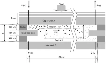
Figure 1 Side view of a generic SPLITT cell.

Split Flow Thin Cell (SPLITT) Separation

C. Contado, University of Ferrara, Ferrara, Italy

Copyright^ 2000 Academic Press

Introduction

SPLITT fractionation (SF) is a relatively new family of separation techniques primarily}but not exclus-ively } applicable to macromolecules and particles. The SF techniques utilize a thin ribbon-shapedSow cell and achieve fractionation by differential trans-port across the thin (transverse) axis of the cell. Since the cell is only a few hundred micrometres thick, the separation path_}which may be less than the nominal channel thickness}is extremely short and the separ-ative transport is correspondingly rapid. Separation is typically accomplished in only a few minutes. This is a particularly valuable feature for example for fragile species that must be fractionated rapidly to avoid degradation (e.g. biological samples). TheSuid that carries dissolved or suspended components through the SPLITT cell is divided at both ends by thinSow splitter elements (seeFigure 1). The inlet splitter ele-ment allows for the smooth merging of two incoming laminae, one carrying the suspended feed material and the other generally containing only the pure

car-rier liquid. Differential transport of feed components between the two laminae (after they are brought into contact) then occurs as a result of a transverse driving force or gradient. At the outlet end, the Sowing liquid volume is divided at a predetermined position by a second splitter element, thus producing two sub-streams that are enriched or depleted in the desired components as a result of the differential transport.

Both preparative and analytical fractionation pro-cess can occur in the SPLITT cells, depending on the injection procedure. A continuous (CSF) process of feeding the cell is advantageous for preparative frac-tionation (gram, kilogram), offering rapid through-put, minimum holdup volumes, and a sharp separ-ative cut off; examples of continuous fractionation can be found in the separation of mineralogical, in-dustrial and food samples.

examples of quantitative determinations include diffusion coefRcients of proteins, settling velocity and the relative content of oversized particles above a cutoff diameter in a particulate material. Moreover because of its ease of theoretical interpreta-tion, the SPLITT cell can be used for the rapid measurement of transport-related properties such as particle size and particle size distribution. The throughput of SF is proportional to many vari-ables such as the sample concentration in the feed stream, the volumetric_Sow rate of the sample stream, the applied _Reld strength and the SPLITT cell area. For preparative applications there is obviously a trade-off between the resolution and throughput in the operation of SF: maximizing the throughput and maintaining an acceptable resolution is the common choice.

The effectiveness of the SPLITT process can be modulated by simply varying the Sow rates of the inlet and outlet substreams, which determine the position of the inlet splitting plane (ISP) and the outlet splitting plane (OSP) and controlling the thick-ness of the transport region; sometimes, unwanted displacements of a few tens of micrometres may be dif_Rcult to discern but they are suf_Rcient to interfere with effective separation. In some cases, the ef_Rciency of the SPLITT process can be controlled by altering the strength of theReld or gradient driving the separ-ative transport.

The efRcacy of SF separation depends instead, on the hydrodynamic integrity of the SPLITT cell. Effec-tive separation is based in fact, on two central re-quirements:

E there must be no hydrodynamic mixing across stream planes; and

E the splitters must be absolutely perfectly aligned so that they are capable of splitting the_Rlm of_Sowing liquid evenly along the stream plane.

Success in fulRlling these requirements is not easy to judge because of the thinness of the cell and the shortness of the transport path.

The selectivity of SPLITT fractionation comes from the applied force. The principal transverse driving forces used include gravity, centrifugation, diffusion, electrical potential gradients, magnetic gradients and hydrodynamic lift forces. The geometry of all the different cells is similar to that depicted in Figure 1, except for the curvature characteristic of the centrifu-gal SPLITT cell.

The simplicity of the SPLITT cell leads to rather rigorous theoretical guidelines on the conditions ne-cessary to achieve a given level of separation.

Theory

The theory of separation by SPLITT cell was for-mulated by J. C. Giddings in terms of experimentally controllable Sow rates in the inlet and outlet sub-streams and it has been developed and implemented through the years; SPLITT fractionation theory can now be found in numerous publications. The separ-ation is performed inside a thin channel, where the behaviour of a sample particle depends on the bal-ance between the external force_Reld and frictional forces (as for _Reld _Sow fractionation techniques (FFF)), combined with the action of theSuxes opera-tive within the cell.

In Figure 1 the sample, suspended in a suitable carrierSuid, is introduced through the top inlet aat a predetermined volumetric Sow rate VQ(a). At the same time, pure carrierSuid enters through the bot-tom inlet bat aSow rateVQ(b); where the two inlet streams join to form a single stream we have the ISP. When theSuid stream reaches the end of the channel, it is mechanically divided into two fractions by the outlet splitter.

The differential displacement of the particles oc-curs towards wall B, based on the driving force exerted on each type of particle by the applied_Reld and the frictional resistance offered by the carrier Suid to particle motion. Thus different types of par-ticle occupy different laminae while theSow through the channel displaces them axially towards the outlet end.

The total volumetricSow rateVQ in the channel can be written both in terms of inletSow rates or outlet Sow rates

V_Q"V_Q(a)_#V_Q(b)_"V_Q(a)_#V_Q(b) [1]

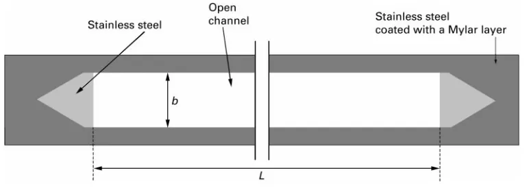
and since the walls A and B are parallel and their dimensions much larger than w (thickness) and b (width), the velocity pro_Rle is essentially two-dimensional (see Figure 2). The mean_Suid velocity vN can be computed asVQ /bw, and the velocity para-bolic proRle across the cell thickness is described by the equation:

v

x w

x

w

x w

wherevmaxis the maximumSuid velocity found at the midplane (x"w/2) of the cell.

By looking at the Sow stream components (see Figure 1) it is possible toRnd a relation which takes into account theSuidSow proceeding in the transport layerVQ(t):

Figure 2 Upper view of the ‘Splitter’ used in the gravitational SPLITT cell. VQ (t) can be obtained by combining eqns [1] and [3]

as:

VQ(t)"VQ (a)!VQ (a)"VQ(b)!VQ(b) [4]

The separation of sample components is achieved, as previously described, by their different rates of transport toward the opposite wall B under the inS u-ence of the transverseReld. It is important to be able to calculate the distance that a component has to travel. The ratio of sampleSow rateVQ(a) to the total Sow rateV_Q de_Rnes the position of the ISP as distance wa, from wall A:

V_Q(a) VQ "3

w2 a_Y w2!2

w3 a_Y

w3 [5]

The feed stream is then con_Rned to the lamina thick-nesswa_Y, between wall A and the ISP.

By assuming that, during their residence in the SPLITT cell, the particles are driven from wall A to wall B at constant velocityU, the volumetricSow rate VQ of the lamina traversed by a particle is simply given by

VQ"bLU [6]

which contains the physical dimensions of the chan-nelb, andL(length);Uis the velocity of the induced transverse transport. In fact, a number of different driving forces have been utilized to implement CSF: gravitational, centrifugal, magnetic, electrical.U as-sumes different expressions depending on the _Reld inducing the transverse transport, i.e.

Ugravitational"gd 2

18o [7]

Ucentrifugal" 2_rd2

18o [8]

U_magnetic"H 2_d

48o [9]

Uelectric"E [10]

wheredis the particle diameter (assumed spherical), is the difference between particle densitys (com-pact particles) and carrier densityl,ois the viscosity of the carrier, g is the acceleration of gravity (earth Reld eqn [7]);is the angular velocity (rad s\1_{) and} ris the radius of the rotation (centrifugal acceleration eqn [8]); is the difference between the magnetic susceptibilities of the particles,p, and the carrier,l, and H is the drop in magnetic Reld strength (eqn [9]); is the electrophoretic mobility and E is the electric Reld strength (eqn [10]). In some cases, experimental studies have been based on diffusive transport or by using hydrodynamic lift forces (which can be used in unique ways because of their nonuniformity).

In order to settle whether particles exit the channel through outlet a or b, the relative values ofVQ and VQ(t) are of critical importance. For a sample intro-duced close to the ISP, particles exit from outlet a if:

VQ)VQ(t) [11]

and from outlet b if:

V_Q'V_Q(t) [12]

In the case of a SPLITT cell operating under a gravitationalReld, the relation which allows one to set the diameter cutoff of a spherical solid particle can be obtained by combining eqns [4], [6] and [7]. In fact, ifV_Q(t)_"V_Q and:

VQ"bLgd 2

then the diameter at which 50% of the particles exit outlet b is called the cutoff diameterdc, expressed as:

dc"

bLg [14]

in which only half ofVQ (a) is considered (cf. eqn [4]). Once dc has been chosen for a given channel, the difference betweenVQ (a) and 0.5VQ(a) is set according to eqn [14]. However, the two constituentsSow rates V_Q(a) andV_Q (a) are not uniquely de_Rned by this equa-tion, but some criteria useful for setting the_Sow rates are available in the optimization of SPLITT opera-tions literature. In general, in order to obtain a separ-ation with a good resolution, the practical rule which states the following necessary but not sufRcient condition:

VQ(b)VQ(a) or VQ(a)VQ(b) [15]

can be followed. This condition ensures that regions I and II will be narrow, which automatically increases the transport region, i.e. the cell space in which the separation process occurs. For maximum resolution, typical experimental conditions, are chosen to obtain aVQ(a)/VQ (t) ratio within 0.1}0.3. From a theoretical point of view, the high resolution in the operative transport mode is, as already stated, contingent on compression of the feed sub-stream, a, into a thin lamina near wall A, and the sharpness of the separ-ation, as in chromatography, can be judged by the numberNof the theoretical plates generated during transport. Generally, for Reld (gravitational) driven migrations, the effectiveNis given by the ratio of two energies:

N"Fwt 2kT"

d3_gw t

12kT [16]

whereFis the force on the particle inducing its trans-port,wtthe length of the transport path, andkTthe thermal energy. Generally values of N*102 _are re-quired to assure achievable resolution, and each type of macromolecule or particle should be checked against this criterion.

Resolution in SF can be related to channel _Sow rates, deRning an index which measures the relative breadth of the unresolved region. It has been demon-strated that for sedimentation particles the equation of the resolving power has the following form:

d1 d"

d1 d1!d0

2 VQ (a)

VQ(a) [17]

whered0andd1are respectively the diameters of the particles exiting from a and b. The particles falling between these two sizes (d1 and d0), which are not fully resolved, exit from both outlets in different proportions, so the difference should be small. Ac-cording to eqn [17] the ratio ofVQ(a) toVQ(a) allows control of the range of unresolved particles which exit both outlets a and b.

Speci

\

c Applications

Determination of the Diffusion Coef\cientD

CSF and ASF can be successfully applied to the separ-ation of macromolecules such as proteins and lipo-somes. The transport region in this case is seen as a diffusion barrier, which acts as a dialysis mem-brane. In order to be able to determine the diffusion coefRcientD, an important parameter useful for char-acterization of the sample components, the theory has to be looked at in a deeper way, with equations which explicitly containD.

If a component enters inlet a as a steady stream and its transport through the SPLITT system is gov-erned by the simultaneous displacements of diffusion and parabolicSow, mass conservation requires that:

c

t"!v(x) c z#D

2_c x2#

2_c

z2

c/t is the rate of change of concentration at an arbitrary point within the channel,xis the transverse distance into the cell measured from wall A,zis the distance into the channel along the length measured from the inlet splitter andvis the local stream velo-city. In order to simplify eqn [18], it can be observed that all transverse transport in the channel occurs by diffusion and that all the components are transported along the cell (z-direction) by convention, so that the diffusion term (D2_c/z2_{) can be neglected.}

Moreover, if the system operates in CSF mode, the component concentrations throughout the cell will attain a steady state, i.e. c/t"0, so that eqn [18] reduces to:

c z"

D v(x)

2_c

x2

wherec(x,z) is subject to the boundary conditions:

c(x, 0)_"co for 0)x)wa_Y c(x, 0)"0 forwa_Y)x)w

In order to calculateD, a dimensionless diffusion time D"Dto_/w2 _{has been developed. The} para-metersto_andw2_{are known becausewisRxed by the} geometry of the channel andto_{is the elution time of} a species dispersed in the total volume of the channel and is related to the totalSow rateVQ by:

to_"V o

VQ " bLw

VQ [20]

whereVo_{is the cell void volume expressed as a} prod-uct of channel dimensions b, L and w. The dimen-sionless time parameterto_{is thus related toD,VQ , and} the channel dimensions by:

D"Dt_w2o" DbL

wV_Q [21]

ConsequentlyDis given by:

D"wVQ D

bL [22]

This equation is used to obtain experimental D values, once _D is found. The total procedure re-quires the following steps: (i) to compute theoretically the concentration proRlec(x,L) over the lateral coor-dinatexat outlet (z"L) by using the Crank} Nicol-son numerical method. In this way, the retrieval of a component at each outlet substream Fa(in i) and Fb (in ii) can be calculated from c(x, L); (ii) to construct a graph of FaversusDfor differentVQ (a)/VQ ratios; (iii) to determine experimentally the retrieval factor at outlet sub-stream a (Fa) from the relative strength of the detector signal (this value depends on theSow ratioVQ(a)/VQ used in the experiment); (iv) to compute the correspondent_Dvalue from the graph Fa versusD byRnding the correspondence between the experimental and theoretical Favalues; (v) to use eqn [22] to calculate D using the D value, and the geometrical dimensionsb,L,wandVQ.

Effect of Particle Shape and Density in the Gravitational SPLITT

The SPLITT cell has been largely applied for the separation of environmental samples. Since the natu-ral matter particles have different properties (poros-ity, dens(poros-ity, shape), the basic SPLITT equations have to be revised toRt the relevant particle properties.

The basic relationship for the SPLITT cell, pre-viously derived (see eqn [6]) can be written as:

VQ"VQ(t)"bLUgravitational [23]

By recalling the basic properties of the sedimentation process different expressions can be obtained, which contain the density parameter. During the SPLITT fractionation, under a gravitationalReld, the sample components are subject to two forces: the gravi-tational force Fg"meffg and the frictional force Ff"fU(meff is the effective mass, and f the friction coefRcient). Usually, the stationary state is estab-lished very rapidly and the two forces balance each other out and thus:

U"meff g

f [24]

Spherical particles In the case of compact spherical particles, by assuming that the particles do not under-go any shrinking or swelling meff"m!mb or meff"Vss!Vsl, where m is the real mass and mbthe buoyant mass whileVsandsare, respectively, the volume and density of the particle and l the density of the liquid. More explicitly

meff"1

6d3 [25]

The accounts for positive or negative mass values in eqn [25] corresponding, respectively, to a falling or a Soating particle. The friction coefRcient f can be expressed by Stokes law f"3d, where is the viscosity of the suspension Suid, which can be ap-proximated by the carrier viscosity,0. By combining eqns [23], [24] and [25] one obtains the classical expression (see eqn [13]):

VQ(t)"bLgd 2

18o [26]

In the case of porous particles, porosity is deRned as:

" Vp Vs#Vp"

Vp Vp

tot

[27]

whereVpis the volume of the pore,Vsthe volume of the solid and Vp

tot the total volume of the particle. Then eqn [25] changes into:

meff"1

6d3(1!) [28]

and the correspondent eqn [26] into:

VQ(t)"bLgd

2_(1!)

The porosity can be expressed also in terms of ‘appar-ent density’:

app"(1_!)_s#l [31]

from which the differential apparent density is de-Rned as:

app"app!l [32]

By combining"s!l with eqns [31] and [32] one has:

app"(1!) [33]

which can be substituted in eqn [30]. When the ‘mass porosity’ is available:

p"Vp

m [34]

wheremis the real mass of the particle, i.e.m"Vss and by using eqn [27] one can show that:

ps#1

which gives:

V_Q (t)_"bLgd 2

18o

1

ps#1

Alternatively, one can employ the ‘bulk density’, which is the ratio between the amount of the porous material, mtot, and the total volume occupied by the packed particlesVtot, including both the inter-particle volume,Vex, the particle volumes, Vtotp (total volume of the pores) andVtot

s (total solid volume):

bulk" mtot Vtot

p #Vtots #Vex" mtot Vtot

[37]

In this instance, both thebulkandexdepend on the degree of packing. The relative apparent density, app can be obtained by combining eqns [33] and [37]:

app" bulk

s(1!ex) [38]

From eqn [33] it is apparent that, in this case, one must know the value of _ex under the same experi-mental conditions which_bulkwas determined. Lack-ing this information, it is only possible to make a rough estimate ofapp.

Nonspherical particles There are two main effects to be accounted for with nonspherical particles: the Rrst is related to the particle volume expression and the second to Stokes Law. The parameterdcontained in eqn [7] has to be changed depending on the kind of data available.

TheRrst effect is accounted for by using the volume equivalent diameter, i.e. the diameter of a sphere having the same particle volume VSp, i.e. d_v"3_((6V

Sp/) instead of the sphere diameter, d. This quantity sometimes can be related to true geo-metrical dimension of the particle if its geometry is known.

An irregular shape affects the behaviour of the particle while it is moving within the Suid. Stokes Law takes account of this by substituting the dia-meterdwith the ‘drag diameter’, i.e. the diameter of a sphere having the same resistance to the motion within theSuid

f"3 odd [39]

In order to conclude this section, an appropriate combination of all the above cases is necessary for irregular porous particles.

List of Symbols

a "aspect ratio

b "width of the SPLITT channel d "diameter of the sphere dc "cutoff diameter dd "drag diameter

dv "diameter of an equivalent sphere D "diffusion coefRcient

E "electrical Reld f "frictional coefRcient

Fa "retrieval of a component from outlet a Fb "retrieval of a component from outlet b Fg "gravitational force

Ff "frictional force g "gravity acceleration

h "thickness of the transport layer hc "high of a cylindrical particle L "length of the SPLITT channel m "real mass of a particle mb "mass corrected for buoyancy meff "effective mass

mtot "total mass of all particles present in the container

p _"mass porosity r _"radius of rotation

U "particle migration velocity vN "meanSuid velocity vmax "maximumSuid velocity

VQ "total volumetricSow rate through cell VQ(a)"volumetricSow rate at outlet a VQ(b)"volumetricSow rate at outlet b VQ(a) "volumetricSow rate at inlet a VQ(b) "volumetricSow rate at inlet b

VQ(t) "volumetric Sow rate of the transport region

Vex "external volume between particles Vp "pore volume of a particle

Vtot

p "total pore volume for all the particles Vs "volume of the solid part of a particle Vtot

s "total solid volume for all the particles VSp "volume of a sphere

Vtot "total volume occupied by all particles present in the container

Vp

tot "total volume of a particle w "thickness of the SPLITT channel

wa_Y "thickness of the Suid lamina between wall A and ISP

wt "thickness of the transport region l "magnetic susceptibility of the carrier p "magnetic susceptibility of a particle "internal porosity

"suspension viscosity o "carrier viscosity

"electrophoretic mobility app "apparent density bulk "bulk density

l "density of the liquid

s "density of the spherical particle "angular velocity

D "dimensionless diffusion time

See also: II/Particle Size Separation: Field Flow Frac-tionation: Electric Fields; Theory and Instrumentation of Field Flow Fractionation. III /Polymers: Field Flow Fractionation.

Further Reading

Allen T (1981)Particle Size Measurement, 3rd edn. Lon-don: Chapman and Hall.

Contado C, Dondi F, Beckett R and Giddings JC (1997) Separation of particulate environmental samples by SPLITT fractionation using different operating modes.

Analytica Chimica Acta345: 99}110.

Contado C, Riello F, Blo G and Dondi F (1999) Continuous split-Sow thin cell fractionation of starch particles. Jour-nal of ChromatographyA 845: 303}316.

Dondi F, Contado C, Blo G and Martin SG (1988) SPLITT cell separation of polydisperse suspended particles of environmental interest.Chromatographia48: 643}654. Fuh CB and Giddings JC (1995) Isolation of human blood cells, platelets, and plasma proteins by centrifugal SPLITT fractionation. Biotechnology Progress 11: 14}20.

Fuh CB and Giddings JC (1997) Separation of submicron pharmaceutic emulsion with centrifugal split-Sow thin (SPLITT) fractionation.Journal of Microseparation9: 205}211.

Fuh CB and Chen SY (1998) Magnetic split-Sow thin frac-tionation: new technique for separation of magnetically susceptible particles.Journal of ChromatographyA 813: 313}324.

Fuh CB, Levin S and Giddings JC (1993) Rapid diffusion coefRcient measurements using analytical SPLITT frac-tionation: application to proteins.Analytical Biochemis-try208: 80}87.

Levin S, Myers MN and Giddings JC (1989) Continuous separation of proteins in electrical split-Sow thin (SPLITT) cell with equilibrium operation. Separation Science and Technology24(14): 1245}1259.

Provder T (ed.) (1991)Particle Size Distribution.II. Assess-ment and Characterization. ACS Symposium Series 472. Washington DC: American Chemical Society.

Yong J, Kummerow A and Hansen M (1997) Preparative particle separation by continuous SPLITT fractionation.

Journal of Microseparation9: 261}273.

Zhang J, Williams PS, Myers MN and Giddings JC (1994) Separation of cells and cell-sized particles by continuous SPLITT fractionation using hydrodynamic lift forces.

Separation Science and Technology29(18): 2493}2522.

Theory and Instrumentation of Field Flow Fractionation

J. Janc\a, Universite& de la Rochelle, La Rochelle, France

Copyright^ 2000 Academic Press

Principle

Field-_Sow fractionation (FFF) is one of the important analytical methodologies, suitable for the separation and characterization of particles in the submicron