A. IfPA , graph G is called compact graph. Compact graph can be seen as



ABSTRACT—Doubly stochastic matrix has many important applications, and the family of compact graphs has important research value which can be seen as the generalization of the famous Birkhoff theorem of doubly stochastic matrix in combinatorial matrix theory. Determining whether a graph is a compact graph is a difficult problem, and only few compact graphs are known at present. We have studied the compact graph and have obtained some results: the graph constructed by the disjoint union of any compact graph and some isolated points is a compact graph, the graph constructed by adding one pendant edge to each vertex of any compact graph is also a compact graph, and some compact graphs also are obtained using above results. In this paper, based on previous studies, the results of compact graphs are further given: the graph constructed by adding

n

pendant edges to each vertex of the complete graph is a compact graph, and the graph constructed by adding two pendant edges to each vertex of any compact graph is a compact graph. The disjoint union of any number of non-isomorphic complete graphs is a compact graph. Combined with these results, some results of compact graphs and super-compact graph are given.

Index Terms—Compact graph, doubly stochastic matrix, super compact graph, permanent

I Introduction

N this paper, the simple and undirected graph

)

,

(

V

E

G



n with the vertex set

V

n



{

1

,

2

,



,

n

}

and

the edge set

E

is considered. The adjacency matrix

)

(G

A

A



of a graph

G

is a (0,1) matrix of order

n

, whose element is

a

_ij



1

or

0

, if an edge



i

,

j



E

or not. Thus, a graph of order

n

corresponds to an adjacency matrix

A



 

a

_{ij nn}. The graphs

G

and

H

are isomorphism if and only if their adjacency matrices are permutation similarity. That is, if

A

and

B

are the adjacency matrices of the graphs

G

and

H

respectively, then

G

and

H

are isomorphism if and only if there exists a permutation matrix

P

such that

AP



PB

, where

P

is called the self-isomorphic permutation matrix of

A

.

Let

p

_n be the set of all permutation matrices of order

n

,

Manuscript received November 07, 2018; revised July 16, 2019. This work was supported by the Foundation of Research Program of Science and Technology at Universities of Inner Mongolia Autonomous Region in China under Grant No. NJZZ18154 and Science Research Fund of Inner Mongolia University for Nationalities in China under Grant No. NMDYB1748 and No.NMDYB19056, Research Topics of Education and Teaching in Inner Mongolia University for Nationalities under Grant No. YB2019016.

Wang Jing-yu is with the Inner Mongolia University for Nationalities, Tongliao 028043 P.R. China.

Siqinbate is with the Inner Mongolia University for Nationalities, Tongliao 028043 P.R. China (corresponding author phone: +86 13947545110; e-mail: siqinbate_828 @163.com).

and

P

(

A

)

be the set of all self-isomorphism of graph

G

, i.e.,

P

(

A

)



{

X

|

X



P

_n

,

AX



XA

}

.

Let

P

(

A

)

denote

















|

1

,

P

(

),

0

)

(

P

A

c

_i

P

_i

c

_i

P

_i

A

c

_i .

A non-negative square matrix

X

is called doubly stochastic matrix, if the

X

is the solution of the Linear programming equation

Xe



X

T

e



e

, where

e

is the

n

-dimensional vector whose elements are all 1.

Let



_n be the set of all doubly stochastic matrices of order

n

, and

}

,

|

{

)

(

A



X

X





n

XA



AX



.

Obviously,

P

(

A

)





(

A

)

. If

P

(

A

)





(

A

)

, graph

G

is called compact graph. Compact graph can be seen as the generalization of Birkhoff theorem[1] of doubly stochastic matrix in combinatorial matrix theory.

Theorem 1.1.(Birkhoff theorem) [1] Let

A

be a doubly stochastic matrix of order

n

, then

A

can be expressed as the convex linear combination of several permutation matrices of order

n

, i.e.

t i i i

A





c P

,

where

P

_i is the permutation matrix of order

n

, t i

1

i

c





,

and

c i

_i

( 1,2, , )





t

is positive.

Let

G

be a complete graph of order

n

, then its adjacency matrix

A J I

 

n n, where

J

n is a square matrix whose all

elements are 1. It is easily to be seen that



( )

A

 

_n and

n

A

)

P

(

P



. S_{o, they are equivalent that}

P

(

A

)





(

A

)

and Birkhoff theorem. Therefore, the compact graph is indeed the extension of the Birkhoff theorem. Birkhoff theorem can be obtained by compact graph.

Theorem 1.2.( Tinhöfer theorem) [2] The disjoint union of the same compact graph is compact graph.

By the definition of compact graph,

K

₂(Complete graph of order two) is compact graph. By theorem 1.2, if

G

is the disjoint union of

n

copies of

K

₂, then

G

is compact graph, and its adjacency matrix is

0

0

I

A

I





 







.

It is easily to be seen that

Some Results of The Compact Graph

Wang Jing-yu , Siqinbate

I

IAENG International Journal of Applied Mathematics, 49:4, IJAM_49_4_26

1 2 3 4

X

X

X

X













0

0

I

I













0

0

I

I





 







1 2 3 4

X

X

X

X













,

if and only if

1

= ,

4 2

=

3

X X X X

.

Let

X S T

 

be a doubly stochastic matrix of order

n

, where

S T

,

are non-negative matrices, then

( )

S T

A

T S















.

By the compactness of

G

, the following results hold

(1) (2) (2) (1) 1

=

t i i i

i _{i i}

S T

P

P

c

T S



P

P



























,

(1) (2)

(2) (1)

( )

i i

i i

P

P

P A

P

P















,

where

c i

_i

( 1,2, , )





t

is positive number and t i

1

i

c





.

If

P P

_i



_i(1)



P

_i(2)

( 1, 2, , )

i





t

, then

P

_i is permutation matrix for all i and t _{i i}

i

X





c P

. It is truly Birkhoff theorem.

Let

A

be the adjacency matrix of graph

G

. If there exists a non-negative square matrix

X

such that

XA AX



, then the

X

is called the non-negative self-isomorphism of

A

. All non-negative self-isomorphisms of

G

are denoted by

)

(

A

Cone

X

XA

AX

X

|

,

{





is a non-negative matrix

}

.

The self-isomorphic set

P

(

A

)

of

G

generates

}

0

),

(

P

|

{

)

(

Pˆ

A





c

_i

P

_i

P

_i



A

c

_i



.

It is easily to be seen that

Pˆ

(

A

)



Cone

(

A

)

. Then, for what kind of graph does the equation

Pˆ

(

A

)



Cone

(

A

)

hold? A graph

G

is called super-compact graph if its adjacency matrix

A

satisfies

Pˆ

(

A

)



Cone

(

A

)

. Obviously

(A)

Pˆ

)

(

P

A



,



( )

A



Cone A

( )

, and it can be proved that if the adjacency matrix

A

of the graph

G

satisfies

)

(

)

(

Pˆ

A



Cone

A

, there must be

P

(

A

)





(

A

)

. So a super-compact graph must be a compact graph. But not all the graphs are compact graphs and the compact graphs are not necessarily super-compact graphs. Sometimes there is little difference between the non-compact and the compact and the super-compact . We will illustrate this in the following.

In 1986, the concept of compact graph is proposed by G.Tinhöfer[2]. In 1988, R.A.Brualdi systematically introduced the compact graph in [3]. In 1990, Bai-lian Liu related some results on the compact graph and gave some new results in [4]. In 1997, C.D.Godsil discussed the compact graph on the view of algebraic combination in [5]. After that, Xiu-ping Zhang and Wei-cheng Lu gave some methods of constructing compact graph in and some results in [6], [7],

[8], [9],[10]. But until now, only few families of compact graphs are known. We have studied the compactness of a graph in [12-14]. Particularly, the following two important results are given in [13] :

Theorem 1.3.[13] The disjoint union of any compact graph and some isolate vertices is compact graph.

Theorem 1.4.[13] The graph obtained by attaching one pendant edge to each vertex of compact graph is compact.

Based on the above results, we obtained some useful results such as any wheel graph is compact graph and any windmill graph is compact graph.

In this paper, based on the previous research, the following results will been given: the graph obtained by attaching

n

pendant edges to each vertex of a complete graph is compact graph, and the graph obtained by attaching two pendant edges to each vertex of any compact graph is compact graph, and the disjoint union of any number of non-isomorphic complete graphs is a compact graph. The relations between non-compact graph and compact graph and super-compact graph will be discussed.

II Definitions and preliminary lennas

Definition 2.1. [4] The maximum number of non-zero elements in different rows and different columns of a nonnegative matrix is called the term rank of the matrix.

Definition 2.2. [4] Let

A



 

a

_{ij m n}

(

m n



)

be a matrix, we call

1 2 1 2

1 2

, , , n m m m

i i mi i i i P

PerA

a a

a











the permanent of

A

, where

P

_mn presents the set of all permutations of

m

elements in



1,2, ,



n



.

Lemma 2.1. [4] The permanent of doubly stochastic matrix is positive.

Lemma 2.2.[4] If the graph

G

is compact, then the complementary graph

G

c of

G

is compact.

Lemma 2.3.[4] The complete graph

K

_n, circle graph

C

_n, tree graph

T

, bipartite graph

K

n n, and graph

K

n n, are all

compact graphs, where

K

n n, is the graph obtained by deleting

1 factor from

K

n n, .

Lemma 2.4.[9] A graph

G

is a super compact graph if and only if

G

is a compact and connected regular graph.

Lemma 2.5. [10] Let

G

₁ and

G

₂ be connected

k

-regular compact graphs of order

n

and

m

respectively,

V

(

G

₁

)







)

(

G

₂

V

,

u

be a vertex of

G

₁,

v

be a vertex of

G

₂ , then the graph

G

obtained by adding edge

uv

to the graph

2 1

G

G



is also compact where

n



m

.

Lemma 2.6.[11] Let



( )

G

be the minimum degree of the vertex of graph

G

with order

n

. If

( )

1

2

n

G





 

 



 

, then

G

is a connected graph.

Lemma 2.7. A non-negative matrix must be a square

IAENG International Journal of Applied Mathematics, 49:4, IJAM_49_4_26

matrix, if its row sum equals to its column sum but not equals to zero.

Proof. Let

A a



( )

_{ij n m} , and the row sum and column

sum be both

r

( 0)



, then ₁

2

m

i ij

j

a

r

a



 



. Hence

1

1 1 2

n n m

i ij

i i j

a

nr

a

  









1

1 2 1

n m n

i ij

i j i

a

nr

a

  











(

1)

r nr m

r

n m

 





 

.

Therefore,

A a



( )

_{ij n m} is a square matrix.

Lemma 2.8. Let

G

be a compact graph of order

n

and its adjacency matrix be

A

,

X



( )

A

,

X S T

 

, where

,

S T

are non-negative matrices, then there are permutation matrices

P

₁

,

P

₂

,



,

P

t



P

(

A

)

such that

t i i i

X





c P

，

(1) (2) (2) (1) 1

=

t i i i

i i i

S T

c

P

P

T S



P

P



























,

where

(1) (2) (2) (1)

i i

i i

P

P

P

P













is a permutation matrix of order

2n

,

(1) (2)

i i i

P P





P

,

c i

_i

( 1,2, , )





t

are positive numbers and t i

1

i

c





.

Proof. Let

Y

S T

T S





 







, by lemma 2.1, the term rank

2

Y

n





. We use mathematical induction on the numbers

( )

Y



of non-zero elements of

Y

.

(i) If



( ) 2

Y



n

, then

X Y

,

are permutation matrices. Lemma 2.8 holds.

(ii) If



( ) 2

Y



n

. Since

X



( )

A

and

G

is a compact graph, so there is a permutation matrix

P

₁



P

(

A

)

such that the positive elements of

P

₁ correspond to the

n

positive independent vectors of

X S T



+

. Decompose

P

₁ into the sum of two matrices

P

₁(1),

P

₁(2) whose elements are 0 and 1 such that the positive elements of

P

₁(1) correspond to the positive elements of

S

, the positive elements of

P

₁(2) correspond to the positive elements of

T

.So

(1) (2) 1 1

(2) (1) 1 1

P

P

P

P













is a permutation matrix and its positive elements group correspond to the independent group of

2n

positive elements

of

S T

T S













:



a a

1j1

,

2j2

, ,



a

2 ,n j2n



.

Denote

c

₁



min



a a

₁j₁

,

₂j₂

, ,



a

_{2 ,}n j_2n



, then

1

0



c

₁



. Let

(1) (2) 1 1 2 1 1 2 1 (2) (1)

1 1 1 1

1

(

),

1

(

)

1

1

P

P

X

X c P Y

Y c

c

c

P

P











 











then

X

₁



( )

A

and

Y

₁ are all doubly stochastic matrices, and

(1) (2)

2 1 1 1 1 1 1

1 1 1

1

(

)=

1

(

)

1

(

)

1

1

1

X

X c P

S c P

T c P

c

c

c

















1

( )

Y

( ) 2

Y









Let _{2 1 1}(1) _{2 1 1}(2)

1 1

1

(

),

1

(

)

1

1

S

S c P

T

T c P

c

c













,

then

X

₂



S T

₂



₂.

If



( ) 2

Y

₂



n

, then make

P

₂



P

(

A

)

such that the positive elements of

P

₂ correspond to the independent group of

n

positive elements of

X

₂



S T

₂



₂. Decompose

P

₂ into the sum of two matrices

P

₂(1),

P

₂(2) whose elements are 0 and 1 such that the positive elements of

P

₂(1)correspond to the positive elements of

S

₂ and the positive elements of

(2) 2

P

correspond to the positive elements of

T

₂ . So

(1) (2) 1 1

(2) (1) 1 1

P

P

P

P













is permutation matrix, and its positive

elements group correspond to the independent group of

2n

positive elements of ₂ 2 2

2 2

S

T

Y

T

S





 







:



(1) (1) (1)



1 2 2

(1) (1) (1) 1j 2j

, ,

2 ,n jn

a a



a

.

Denote



(1) (1) (1)



1 2 2

(1) (1) (1) 2

min

_1j

,

_2j

, ,

_{2 ,n jn}

c



a

a



a

,

then

0



c

₂



1

. Let

(1) (2) 2 2

3 1 2 2 3 1 2 (2) (1)

2 2 2 2

1

(

),

1

(

)

1

1

P

P

X

X c P Y

Y c

c

c

P

P











 











3 2

( )

Y

( ) 2

Y









,

then

X

₃



( )

A

and

Y

₃ are all doubly stochastic matrices. Repeating the above process, the following iterative formula can be got:

1 1 1 1

,

;

,

,



 









 

 











X X X

S T

S T

Y Y Y

T S

IAENG International Journal of Applied Mathematics, 49:4, IJAM_49_4_26

1 1 1

1

(1) (2)

1 1 1 1 1 1

1 1

(1) (2) 1 1 1 1 (2) (1)

1 1

1

1 1 1 1

,

1

,

( 2,3, );

1

1

( 2,3, ),

1

=

(1

i i i

i i i

i

i i i i i i

i i i i i i i i i i i i i i i i

i i i i

X

c P

X

S T

c

S

c P

T

c P

S

T

i

c

c

P

P

Y

c

S T

P

P

Y

i

T S

c

X

c P

c

                      







 







































































 







(1) (2) 1 1

1 1 (2) (1) 1

1 1

) ( 2,3, );

(1

) ( 2,3, ),

i

i i

i i i i

i i

X i

P

P

Y

c

c Y i

P

P

      















 



















where

P

_i₁



P

_i(1)₁



P

_i(2)₁

; ( )



Y

_i





( ) 2( 1).

Y



i



Since

Y

_i is doubly stochastic matrix, there is a

t

such that

( )=2

Y

_t

n



, i.e.,

Y

_t is permutation matrix. So by

i i i

X

 

S T

, we know

X

_t is also permutation matrix.

Let (1) (2) (2) (1) t t t t t

P

P

Y

P

P





 







, then

(1) (2)

=

+

t t t

X P

P

,

X

_t is

denoted by

P

_t . Iterating the above formula, there is

0( 1,2,3, , )

i

c



i





t

,

=1

1

t i i

c





such that

1 1 2 2 3 3

(1) (2) (1) (2) 1 1 2 2 1 (2) (1) 2 (2) (1)

1 1 2 2 (1) (2) (1) (2) 3 3

3 (2) (1) (2) (1) 3 3

=

;

=

,

t t t t t t t

X c P c P c P

c P

P

P

P

P

Y c

c

P

P

P

P

P

P

P

P

c

c

P

P

P

P





 















































 





 























In summary, Lemma 2.8 holds.

III Main results and their proof

Let

G

be any graph and

G

 be the graph obtained by attaching

n

pendant edges to each vertices of

G

. Let

A

be the adjacency matrix of graph

G

, then by adjusting the order of vertices, we can obtain the adjacent matrix of

G



0 0

0

0 0

0

0 0

0

A I I

I

I

A

I

I











































    



.

Let

X

 be the doubly stochastic matrix with the same order as

A

. Perform the same partitioned mode of

X

 as

*

A

such that

12 13 1, 1 21 22 23 2, 1 31 32 33 3, 1

1,1 1,2 1,3 1, 1

n n n

n n n n n

X

X

X

X

X

X

X

X

X

X

X

X

X

X

X

X

X

        





















































If

A X

 



X A

 , then

12 21 13 31 1, 1 1,1

2 3 , 1 2 3 1,

= = =

;

;

+

( 2,3, ,

1);

+

(

2,3, ,

1).

n n

i i i n

j j n j

X X X X

X

X

Y

AX XA

YA X X

X

X i

n

AY X X

X

X j

n

   

 













 

 













 



















Since

X

 is doubly stochastic matrix, the row sum of

1 2

n ik k

Y



X







equals to the row sum of

X nY



. Hence the

row sum of 1

2 n ik k

X

 



is equal to or larger than the row sum of

X

. Since

YA



0

, and

1 2

( 2,3, ,

1)

n

ik k

YA



X

X i

n















,

we know

YA

=0

. Thus 1

2

( 2,3, ,

1)

n

ik k

X

X i

n















.

Also, the row sum of 1

2

n ik k

Y



X







and

X nY



are all equal to 1, so if

n



2

, then

Y

=0

. Therefore,

22 23 2, 1 32 33 3, 1

1,2 1,3 1, 1

0

0

0

0

0

0

n n

n n n n

X

X

X

X

X

X

X

X

X

X

X

      





















































, 1 2 1 2

;

(

2,3, ,

1);

(

2,3, ,

1).

n ik k n jk k

XA AX

X

X i

n

X

X j

n

   







































(*)

Whereas, if

X

 satisfies the condition (*), then

A X

 



X A

 

.

If

G

is complete graph, then



( )

A

 

_n . Obviously,

the condition

XA AX



in (*) can be satisfied. Hence for complete graph

G

and the null graph

G

₀ with same order (Constructed by some isolated vertices), we have

0

( )

A



( )

A





 

, _where

A

 _and

A

₀_{are the adjacency}

matrices of

G

 and

G

₀ respectively. Since

G

₀ is the disjoint union of the same star graph, and the star graph is

IAENG International Journal of Applied Mathematics, 49:4, IJAM_49_4_26

compact[4]_{, by theorem 1.2,}

0

G

 _{is a compact graph. So}

G



is also a compact graph and the following theorem holds: Theorem 3.1. The graph obtained by attaching

n

pendant edges to each vertices of complete graph is a compact graph. Whether the result similar as theorem 3.1 holds for any compact graph? It is an unsolved problem. For the special case, we give the following theorem after theorem 1.4:

Theorem 3.2. The graph obtained by attaching two pendant edges to each vertices of any compact graph is a compact graph.

Proof. Let

G

be a compact graph of order

n

,

A

be the adjacency matrix of

G

,

G

* be the graph obtained by attaching two pendant edges to each vertices of

G

, and

A

* be the adjacency matrix of

G

*. By properly adjusting the order of the vertices, we can make

0 0

0 0

A I I

A

I

I











 











Let

X





( )

A

 . Perform the same partitioned mode of

X



as

A

* such that

12 13 21 22 23 31 32 33

X

X

X

X

X

X

X

X

X

X











 











Since

A X

 



X A

 , combining with above discussion, we know

22 23 32 33

0

0

0

,

0

X

X

X

X

X

X











 











2 3 2 3

;

+

(

2,3);

+

(

2,3).

i i

j j

XA AX

X X

X i

X

X

X j





















Hence

X

₂₂

=

X

₃₃

,

X

₃₂

=

X

₂₃ . Let

X

₂₂

= ,

S X

₃₂

=

T

, then

0 0

0

0

X

X

S T

T S











 











,

where

X



( )

A

,

S T

T S













is doubly stochastic matrix of

order

2n

, and

X S T

 

.

Since

G

is a compact graph, by lemma 2.8, we have

1

t i i i

X

c P







,

1

1

t

i i

c







,

P

_i



( )

A

 . So

G

* is a compact graph.

From lemma 2.4 and theorem 3.2, the graph obtained by adding two pendent edges to each vertex of any super-compact graph is a compact graph, but not a super --compact graph.

Theorem 3.3 The disjoint union of any number of non-isomorphic complete graphs is a compact graph.

Proof. Let

G

be the disjoint union of the

n

distinct complete graphs

G G

1

, , ,

2

L

G

n with the adjacency matrices

1

, , ,

2 n

A A

L

A

_{respectively, where}

A

_{i is the matrix of order}

i

n

. Then the adjacency matrix of

G

is

1 2

( , , , )

n

A diag A A



L

A

_.

Let

X



( )

X

_{ij n n}



( )

A

, then

A X

i ij



X A

ij j,

( ,

i j



1,2, , )

L

n

. Since

A J I

i

 

i i,

A

j



J

j



I

j, so

i ij ij j

J X



X J

. Then the row sum and the column sum of

ij

X

are same. According to Lemma 2.7, when

i j



,

0

ij

X



. Hence

11 22

(

,

, ,

nn

)

X diag X X



L

X

_,

( )( 1,2, , )

ii i

X



A i



L

n

_.

By Lemma 2.3,

G i

i

( 1,2, , )



L

n

are compact graphs.

So there exist

P P A i

i



( )( 1,2, , )

i



L

n

such that the

positive elements of

P

_i correspond to the independent group



( ) ( ) ( )



1 (1)i

,

1 (2)i

, ,

1 ( )i i

i i i

n

x



x



K

x



of the positive elements of

X

ii.

Let



( ) ( ) ( )



1 (1) 1 (2) 1 ( )

min

i_i

,

i_i

, ,

i_{i i} i

x



x



x

 n





L

;





min

_i

|

i

1,2, ,

n









L

;

P diag P P





₁

, , ,

₂

L

P

_n



. (1) If





1

, then

X P

 

( )

A

.

(2) If





1

, let

1 (

)

1

Y

X



P









, then it is

obviously that

Y



( )

A

and

Y

has at least one zero elements more than

X

. Using mathematical induction on the number of non-zero elements, we obtain

X



( )

A

.

In summary,



( )

A

 

( )

A

. That is



( )

A

 

( )

A

, and

G

is a compact graph. [image:5.595.326.513.639.736.2]

Example 3.1. By theorem3.3, the disjoint union of the complete graphs

K

₅ and

K

₆ is a compact graph. And by theorem 3.2, the following graph (Fig 1 Compact graph) is compact.

Fig 1 Compact graph

Theorem 3.4 The disjoint union of circle

C

₃ and circle

(

3)

n

C n



is a non-compact graph.

IAENG International Journal of Applied Mathematics, 49:4, IJAM_49_4_26

Proof. Let

A

be the adjacency matrix of

C

₃,

B

be the adjacency matrix of

C n

_n

(



3)

, then

A J



₃



I

₃ ,

ij n

B

  

 

b

, where

b

_ij satisfies that

b

_ij



1

if

)

(mod

1

n

i

j





or

j



i



1

(mod

n

)

and otherwise

0

ij

b



.

Let

 

1 1





,







1 0 0

L

0 0 0 1



_,

then

1

0

T

A

A









 







, 1

0

T

B

B









 







,

It is easily to be seen that

1

₃

(

( , ))

3

J

n

diag A B

n







.

Therefore, if the disjoint union of circle

C

₃ and circle

(

3)

n

C n



is a compact graph, then

3

1

3

J

n

c P

i i

n









,



c

i



1

,

P

i



(

diag A B

( , ))

.

Furthermore, there must be a permutation matrix

P

whose element

(1,4)

is 1 in



(

diag A B

( , ))

. Let

3 3 3 3

n n n n

P

P

P

P

P

   





 







, 3

1 0

0

n

P

X







 







,

then by

P diag A B



( , )



diag A B P

( , )



, we known

3 3

1 1

1 1 1 1

0

1 0

1 0

0

0

0

,

,

.

.

n n

T T

T T T T

AP

P B

A

X

X

B

X

X

A

B

A X XB

















 

 













 















 











 

































　

However,

 

A

₁ T



2

,

 

B

₁ T



0

,

1 T 1 T

.

A

B

 



 

Hence the disjoint union of circle

C

₃ and circle

C n

_n

(



3)

is a non-compact graph. The proof of Theorem 3.4 is finished.

Since the complete graph

K n

_n

(



1)

is a

n



1

regular connected compact graph, there exists a

n

regular connected compact graph of order

n



1

for any non-negative integer

n

. Therefore, the super-compact graphs of any order exist.

For non-compact graphs, the following conclusions can be drawn from Lemma 2.2 and Theorem 3.4:

Corollary 3.1 If

n



3

, the

n



1

regular connected non-compact graph of order

n



4

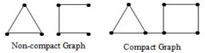
exist.

Sometimes, the difference between a non-compact graph and a compact graph is very small and maybe is only lost one edge, which can be seen from Lemma 2.5 and Theorem 3.4. For example:

Fig 2 Difference between non-compact graph and compact gagraph

[image:6.595.44.294.48.640.2]

Similarly, the difference between the compact graph and the super-compact graph can be only lost one edge, which can be seen from Theorem 1.3, Lemma 2.2, Lemma 2.3 and Lemma 2.4. For example:

Fig 3 Difference between compact graph and super compact graph

The following two conclusions are also notable. Corollary 3.2. For

n



5

,

C

_n and c

n

C

both are

simultaneously super-compact graphs .

Proof. When

n



5

,

( )

3

1

2

c

n

n

C

n



  

 

 



 

, so

c n

C

is a

connected graph. By Lemma 2.2, Lemma 2.3 and Lemma 2.4,

n

C

and c

n

C

both aresimultaneously super-compact graphs . Corollary 3.3. When

n



3

,

K

n n, and

K

n nc, both are

simultaneously super-compact graphs, where

K

n n, is the

graph obtained by deleting 1-factor from

K

n n, .

Proof. Since



(

K

n nc,

)

  

n

1





2

2

n





  

1

n

1





, so

,

c n n

K

is a connected graph. When

n



3

, it is easy to know that

K

n n, is a connected graph by mathematical induction.

By Lemma 2.2, Lemma 2.3 and Lemma 2.4,

K

n n, and

K

n nc,

both aresimultaneouslysuper-compact graphs.

REFERENCES

[1] Birkhoff G, “Tres observaciones sobre el algebra lineal,” Univ.Nac. Tucumàn Rev. Sor. A, vol. 5, pp. 147-150, 1946.

[2] Tinhöfer G, “Gragh isomorphism and theorems of Birkhoff type,” Computing, vol. 36, pp. 285-300, 1986.

[3] Brualdi A R, “Some application of doubly stochastic matrices,” Linear Algebra Application, vol. 107, pp. 77-100, 1988.

[4] Liu Bolian,Combinatorial Matrix Theory. Beijing, Science Press, 2005.

[5] Godsil D C, “Compact graph and equitable partitions,” Linear Algebra Application, vol. 225, pp. 259-266, 1997.

[6] Zhang Xiuping, “Some results on compact graphs and supercompact graphs,” Journal of Beijing Normal University(Natural science), vol. 35, issue 1, pp. 16-21, 1999.

[7] Zhang Xiuping, “The compactness and supercompactness of

Semi-Complement graph,” Journal of Beijing Normal

University(Natural science), vol. 35, issue 3, pp. 316-319, 1999. [8] Zhang Xiuping, “Some results on the compactness and

supercompactness of ( , )m k graph and their Semi-Complement graph,” Journal of Beijing Normal University(Natural science), vol. 36, issue 5, pp. 569-573, 2000.

[9] Lu Weicheng, Zhang Xuanhao, “The Theory of Compact Graph and Supper Compact Graph,” Science Technology And Engineering, vol. 11, issue 11, pp. 2399-2403, 2011.

IAENG International Journal of Applied Mathematics, 49:4, IJAM_49_4_26

[image:6.595.321.523.55.108.2]

[10] Zhang Xuanhao, Lu Weicheng, “A Method of Constructing the Compact Graph,” Science Technology And Engineering, vol. 11, issue 26, pp. 6249-6252, 2011.

[11] Bondy J.A. and Murty U.S.R., Graph theory with applications. London: Macmillan Press, 1976.

[12] Sinqinbate, WANG Jing-yu. “Some Research Results about Compact Graph,” Mathematics In Practice And Theory, vol. 45, issue 7, pp.296-303, 2015.

[13] Sinqinbate, WANG Jing-yu. “Two results of the compact graph and its applications,” Operations Research Transactions, vol. 19, issue 4, pp.72-82, 2015.

[14] Siqinbate, WANG Jing-yu, “The compactness on complete graph,” Mathematics In Practice And Theory, vol. 46, issue 18, pp. 229-234, 2016.

IAENG International Journal of Applied Mathematics, 49:4, IJAM_49_4_26