The calculation of the potential of mean force using computer simulations

ELSEVIER Computer Physics Communications 91 (1995) 275-282

Computer Physics

Communications

The calculation of the potential of mean force using

computer simulations

Beno~t Roux

UniversiM de Montreal, Physics Department, C.P 6128, succ. Centre-Ville, Montrdal, Canada H3C 3J7

Received 10 October 1994

Abstract

The problem of unbiasing and combining the results of umbrella sampling calculations is reviewed. The weighted histogram analysis method (WHAM) of S. Kumar et al. (J. Comp. Chem. 13 (1992) 1011) is described and compared with other approaches. The method is illustrated with molecular dynamics simulations of the alanine dipeptide for one- mad two-dimensional free energy surfaces. The results show that the WHAM approach simplifies considerably the task of recombining the various windows in complex systems.

Keywords:

Computer simulations; Umbrella sampling; Free energy surface; Potential of mean force; Alanine dipeptide

1. Introduction

The potential of mean force (PMF) W ( s c) along some coordinate s ~, first introduced by Kirkwood in 1935 [ 1 ], is a key concept in modern statistical me- chanical theories of liquids and of complex molecu- lar systems. It is defined from the average distribution function (p(s ¢)),

[

W ( s c) = W(~:*) -

kBTln

L ~ J ' (1)

where ~:* and Y¢(~:*) are arbitrary constants. The av- erage distribution function along the coordinate ~ is obtained from a Boltzmann weighted average,

(p(~:)) =

f d R t~

(~:'[R] - s c)

e -U(R)/kBT

f dR

e-U(R)/kBr , (2)

where

U(R)

represents the total energy of the sys- tem as a function of the coordinates R and ~:t[R] is a function depending on a few or several degrees of

freedom in the dynamical system (e.g., stY[R] may be an angle, a distance, or a more complicated function of the Cartesian coordinates of the system). In par- ticular, conformational equilibrium properties or the transition rate of dynamical activated processes can be expressed conveniently in terms of the function W(~:) [2]. For these reasons, the PMF is a central quantity in computational studies of macromolecular systems. It is often impractical to compute the PMF W(~:) or the distribution function (p(s~)) directly from a straight molecular dynamics simulation. For example, the presence of large energy barriers along s ~ may pre- vent an accurate sampling of the configurational space within the available computer time. To avoid such dif- ficulties, special sampling techniques have been de- signed to calculate the PMF from a molecular dynam- ics trajectory effectively. One of these approaches is the umbrella sampling technique of Torrie and Val- lean [3,4]. In this method, the microscopic system of interest is simulated in the presence of an artificial bi-

276 B. Roux / Computer Physics Communications 91 (1995) 275-282

asing window potential, w(sC), introduced to enhance the sampling in the neighborhood of a chosen value s c. The biased simulations are generated using the po- tential energy [U(R) + w(~ c) ]. Typically, the biasing potential serves to confine the variations of the coordi- nate ~: within a small interval around some prescribed value, helping to achieve a more efficient configura- tional sampling in this region (this is the reason why the biasing potential is called a window potential). For example, a reasonable choice to produce the biased en- sembles, though not the unique one, is to use harmonic functions of the form wi(~) = ½ K ( ( - ~i)2, centered on successive values of sci. Because the sampling is confined to a small region during a given biased sim- ulation, only a small piece of the estimated PMF is sufficiently accurate to be useful. To obtain the PMF over the whole range of interest of (, it is necessary to perform a number of biased window simulations, each biasing the configurational sampling around a differ- ent region of s c. Ultimately, the results of the various windows are unbiased and then recombined together to obtain the final estimate W ( ~ ) .

These last steps are the most important in an um- brella sampling calculation. According to Eq. (2), the biased distribution function obtained from the ith bi- ased ensemble is

( P ( ( ) ) ( i ) = e-Wi(()/kBr (P(sc)) (e-W'(()/kBr) - l (3)

The unbiased PMF from the ith window is

W/(~:) = W ( ( * ) -

kBTln

[ ( P ( ( ) ) ( i ) ] (p(sC*)) J

- - w i ( ( ) + Fi, (4)

where the undetermined constant F/defined from

e-F'/k"r = (e--W'(()/~:Br), (5)

represents the free energy associated with introduc- ing the window potential. There have been numer- ous efforts at addressing the problems of unbiasing and recombining the information from umbrella sam- piing calculations. Traditionally, the unknown free en- ergy constants F,. are obtained by adjusting the various Wi (~) of adjacent windows in the region in which they overlap until they match [3,4]; the matching can be done manually or automatically, using a least-squares procedure [ 5]. After the free energy constants have

been obtained, the PMF for the whole range of in- terest is generated by connecting the various W i ( ( )

together and discarding the superfluous data in the re- gion in which they overlap [3,4]. Although this is a valid procedure to construct the PMF, it is very lim- ited in practical applications. For example, a signifi- cant overlap between the adjacent windows is neces- sary to overcome the statistical errors in each individ- ual estimates. Thus a large quantity of the simulation data is not used. Furthermore, because the process of matching the adjacent windows is somewhat arbitrary, the uncertainty involved in the process results in a global error that grows with the number of windows. Additional problems arise in the case of free energy surfaces in a space of higher dimensionality [6], e.g., the value of a free energy constant Fi allowing a best match along one coordinate may differ from that al- lowing a best matching along other coordinates due to statistical fluctuations.

The weighted histogram analysis method (WHAM) proposed by Kumar et al. [ 10] aims at using all the information present in the umbrella sampling simula- tions and avoids the problems mentioned above. One of the main advantages of WHAM is that it can be easily extended to treat the case of a PMF depending on more than one variable [10,11]. The approach represents a generalization of the histogram method developed by Ferrenberg and Swendsen [12]. The central idea, which goes back to the maximum over- lap method developed by Bennet to estimate free energy differences [ 13], consists in constructing an optimal estimate of the unbiased distribution function as a weighted sum over the data extracted from all the simulations and determining the functional form of the weight factors that minimizes the statistical error. The WHAM approach is now routinely used to cal- culate the PMF along a single coordinate [ 10,11,14]. However, no applications of the approach to the case of a multidimensional free energy surface could be found in the literature when this paper was written despite the fact that this represents a straightforward extension of the methodology [ 11 ].

In this paper, we describe and compare different methods to unbias and recombine the results from um- brella sampling calculations. Three different weight- ing methods, the weighted histogram analysis method (WHAM) [ 10], a weighted distribution function (W- DF) [5], a weighted potential of mean force (W- PMF) [9,15] as well as an approach based on free energy perturbation (FEP) [7], are considered. The alanine dipeptide was chosen for a model system and PMF's depending on one and two coordinates were examined.

2. Theory and method

We consider an umbrella sampling calculation in- volving Nw biased window simulations. The WHAM equations express the optimal estimate for the unbi- ased distribution function as a C-dependent weighted sum over the Nw individual unbiased distribution func- tions [ ( p ( g ) ) ] unbiased _{(i) [ 10,12],}

Nw

~"~ [ , (-,-),]unbiased (P(¢))=2_., ~P ¢ ) (0

i=l

nie_[W~(~l_Fd/~r

x [ E ; ~ nJ e-[wA¢)-Fxl/*Br '

(6)

where

ni

is the number of independent data points used to construct the biased distribution function. Based on Eqs. (3) and (5), the individual unbiased distribution function is

[ ( p ( g ) ) l unbiased e+Wi('~)/kaT(p(g))(i)e-Fi/knT J (i) =

(7)

and Eq. (6) can be re-written in the form [ 10,11]

Nw

(p(g) ) = ~ ni(p(g) )(i)

i=l

[z

Nw

]

x

nje -lwj(~)-Fjl/kBr

(8)

L j='

J

The free energy constants

Fi,

needed in Eq. (8), are determined from Eq. (5) using the optimal estimate for the distribution function,

= / dg e-W'(~)/kaT(p(g)).

(9)

e-F~/kaT

Because the distribution function itself depends on the set of constants

{Fj},

the WHAM equations (8) and (9) must be solved self-consistently. In practice this is achieved through an iteration procedure. Starting from an initial guess for the Nw free energy constants F/, an estimate for the unbiased distribution is obtained from Eq. (8). This estimate for ( p ( g ) ) is used in Eq. (9) to generate new estimates for the Nw free energies con- stants F/and a new unbiased distribution is generated with Eq. (8). The iteration cycle is repeated until both equations are satisfied.

Extensions of the method to multidimensional cases is straightforward. For example, in the case of two variables ~:l and g2, Eqs. (6) and (9) become

Nw

(P(gl, g2)) = ~

ni(P(gl,

g2) )(i)

i=l

(lO)

278

e-F'/kBr = / del / de2 e--WJ(¢l'¢2)/kBr (p(1~l,t~2) ) .

(11)

As in the one-dimensional case, the WHAM equa- tions (10) and ( 11 ) are solved self-consistently.

For a comparison with the PMF calculated with WHAM, let us consider the free energy perturbation method (FEP) of Haydock et al. [7]. The central idea of the method is to calculate the free energy difference AFi,i_l between the window potentials

w i

and

Wi_l,

AF/,i_l = F / - F~_I

= -kBT

In [(e -lw'<~:)-w'-' (~) l/kBr)(i-1)] .(12)

An equivalent expression can be written for the back- ward free energy

Fi-l,i.

In one dimension, the con- stants F, can be obtained by recurrence, i.e.,

Fi = F1 + AF2,1 + "" + AFi,i_I.

(13)

Extension of the FEP method to the case of higher di- mensions is relatively straightforward, although it re- quires special care. The relative free energy difference between the adjacent windows can be calculated in two-dimensions using Eq. (12). However, it can be ex- pected that the cumulative free energy resulting from the free energy differences along any closed path is not identically zero due to statistical fluctuations in the sampling; e.g., ~-~'9 °sed path AFi, j =it= O.

ThUS,

the cal- culated free energy differences

AFi,j

may not be con- sistent with a unique set of constant F,. In the present application, a least-squares procedure was used to de- termined a unique set of constants

Fi

from all the rel- ative free energy differences AF/,j between the adja- cent windows. Once the Fi are determined, the PMF's from the individual windows, )4;i, can be generated with the proper offset constants and no supplementary matching is required.

Different approaches have been proposed to com- bine the available data avoiding the discarding of any information. To construct the PMF over the whole range of interest, Shen and McCammon used a weighted sum over the individual unbiased distribu- tion functions extracted the Nw windows [5],

Nw

(p(~:)) =

~[

(p(~:)) ] ~n~iased

i=!

B. Roux / Computer Physics Communications 91 (1995) 275-282

[

ni(p(~))(i)

]

× ~ - ~ , (14)

L~-]j_-i

njIp(~) )(y) J

with a straightforward extension to cases of higher di- mension. In the following, the weighted distribution function procedure is referred to as W-DE The s c- dependent weighted average expressed by Eq. (14) is not unique. For example, Woolf and Roux used a weighted sum over the individual unbiased PMF's )/~i (~) [9,15],

N.

[ Nwni(p(~))(i)

]

w(~) = ~ wi(~)

(15)

i=,

L~j=1

nj(p(~))(j)

with a similar expression for the two-dimensional case. In the following, the weighted PMF procedure is re- ferred to as W-PME Both W-DF or W-PMF can be used to recombine the results from FEE

In fact, the W-DF and W-PMF ~:-dependent weighted sum are very similar to the WHAM equa- tion (6). The three expressions, Eqs. (6), (14) and (15), serve to recombine all available data into a smooth function valid over the whole range of s c. Eq. (6) gives more weight to the ith estimate where the Boltzmann factor of the ith window potential is large whereas Eqs. (15) and (14) give more weight to the estimate of the ith window where the biased distribution (P(~))(i) is statistically more important. This similarity with the WHAM formulation suggests that Eqs. (15) (or Eq. (14) ) and (9) may be solved self-consistently providing a different estimate of the free energy constants F/. To examine the validity of the weighted sums equations (15) and (14) the self- consistent W-PMF and W-DF approaches were also tested.

3. Illustration o f the methods

dimensional) and in the presence of one isolated water molecule (two-dimensional) using the FEP and the self-consistent WHAM, W-PMF and W-DF methods. All the calculations were done including all hydrogen atoms with the CHARMM PARM22 potential func- tion [16] for the peptides and TIP3P [17] for the water.

To first test the methods in a one-dimensional case, the PMF W ( r ) along the N-H...O--C distance r of the alanine dipeptide was calculated in vacuum• The potential energy of the system was biased with a har- monic potential, ½K(r - ri) 2, centered on successive values of ri, where K is the harmonic force constant• The conformational sampling was performed with Langevin dynamics; trajectories of 100 ps were gener- ated for five windows, centered on 1.5, 2.5 . . . 5.5 with a harmonic force constant K of 5 kcal/mol/A 2. A time step of 0.002 ps was used for all simulations and a friction constant of 25 ps -1 was applied to all non-hydrogen atoms• Each window was equilibrated during 10 ps starting from the last configuration of the previous window• The self-consistent set of equa- tions (WHAM, W-PMF and W-DF) were iterated until changes in the free energy constants Fi were less than 0.001 kcal/mol. The free energy differences in the FEP method were calculated by averaging the backward and forward perturbations and the resulting YVi(r) were combined together using Eq. (15). To provide a reference for comparison with the PMF calculated with the umbrella sampling method, a sin- gle unbiased simulation of 2 ns was generated. In the remainder of the paper, the PMF calculated from the 2 ns simulation is referred to as exact.

To illustrate the methods in the case of a two- dimensional free energy surface, the PMF of the Ci-7 hydrogen bond, V V ( r , d ) , was calculated in the presence of a single water molecule at a dis- tance d from the carbonyl oxygen of the C=O group (d is the water hydrogen - carbonyl oxygen dis- tance). The two-dimensional free energy surface was computed using a protocol similar to that described above. The potential energy of the system was biased with two harmonic potentials, centered on succes- sive values of the distances r and d, i.e., w i ( r , d ) =

I g r ( r - r i ) 2 -~- I g d ( d - d i ) 2, w h e r e Kr a n d Ka are the harmonic force constant of the window potential. After equilibration for 10 ps, Langevin trajectories of 100 ps were generated for an eight by eight grid of

2 5 0 0

2 0 0 0

C O

O 1 5 0 0

1 0 o o

E

z 5 0 0

0

1 • 2 . 0

/ ' \ /

3.0 r

4 • 0 5 • 0 6 • 0 ( A n g s )

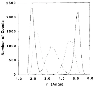
Fig. 1. Histograms generated for each window for calculation of the PMF of the intramolecular hydrogen bond characterizing the Ci-7 conformation. The histograms were calculated with a bin width of 0.1 ,~. A total number of 10000 data was used from the time-series. The average position from each window ( 1 to 5) was 2.05403, 2.41345, 3.44748, 4.62168 and 5.16744/~, respectively. and the rms fluctuation was 0.17047, 0.26313, 0.41399, 0.32528 and 0.19046/~.

windows along r and d, centered on 1.0, 1.5, 2.0 ... 5.5/~ with force constants of 10 kcal/mol//~, 2. The self-consistent set of equations (WHAM, W-PMF and W-DF) were iterated until changes in the free energy constants F/ were less than 0.001 kcal/mol. No stable self-consistent solution could be found with W-PMF. The free energy differences in the FEP method were calculated by averaging the backward and forward perturbations and the resulting VVi(r) were combined together using a two-dimensional extension of Eq. (15).

4. Results and discussion

[image:5.548.292.488.85.268.2]

280 B. Roux / Computer Physics Communications 91 (1995) 275-282

1 , 4 0

1 . 2 0

1 . 0 0 O

E 0 . 8 0

O

.~ 0 . 6 0

u. 0 . 4 0

a. 0 . 2 0

0 . 0 0

- 0 . 2 0 ~ ~ '

1 . 5 2 . 0 2 . 5 3 . 0 r

3 . 5 4 . 0 4 . 5 5 . 0 5 . 5

[image:6.548.289.488.82.280.2]

( A n g s )

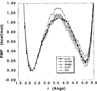
Fig. 2. PMF of the intramolecular hydrogen bond characterizing the Ci-7 conformation. ( r corresponds to the N-H...O=C distance). The PMF's calculated from the unbiased 2 ns simulation (exact), free energy perturbation (FEP), and the self-consistent weighted histogram analysis method (WHAM), the weighted PMF method (W-PMF), and the weighted distribution function (W-DF) are shown. The FEP windows were recombined using Eq. (15). kcal/mol with WHAM and 0.06 kcal/mol with W- PMF in the region of the central barrier. In this region a larger error may be expected because the number of counts in the histogram bins of the biased simulations is smaller; the relative error in the histogram bins is in the order of 1/v/-N, where N is the number of counts [ 10]. The average number of counts is around 2500 for r around 2 and 5/~, whereas it is only 600 around 3.5/~ due to the influence of the central barrier. For comparison, the number of counts in those bins was 1200 for the 2 ns simulation. The convergence in the barrier region could be improved by using an approx- imate guess to the PMF as an overall biasing potential in addition to the successive harmonic window poten- tials, i.e., w i ( r ) = ½ K ( r - ri ) 2 - wguess ( r ) , such that the resulting free energy profile of the system is more uniform [ 18].

The free energy constants Fi used in Eq. (4) to un- bias the individual W i are given in Table 1. Gener- ally, the values calculated with FEP using Eq. (12) and those obtained with WHAM and W-PMF using Eq. (9) are in good accord with the free energy con- stants extracted from the 2 ns unbiased simulation. In the W-PMF method, the best estimate of the PMF is constructed from a linear combination of the individ-

o

O

LI.

a.

1 . 5

1,1

0 . 7

0 . 3

- 0 . 1

- 0 . 5 - -

1 . 0 2 . 0 3 . 0 4 . 0 5 . 0

r ( A n g s )

6 . 0

Fig. 3. Individual Wi from the five windows shown with the final W-PMF estimate.

Table 1

Comparison of the free energy constant Fi Free energy constants (kcal/mol)

Exact WHAM W-PMF W-DF PEP a F1 0.000 0.000 0.000 0.000 0.000 F2 -1.020 -1.027 -1.041 -1.059 -1.095 F3 -0.321 -0.316 -0.358 -0.410 -0.229 F4 -0.715 -0.745 -0.802 -0.874 -0.716 F5 -0.437 -0.467 -0.525 -0.597 -0.403 aCalculated from an average of the forward and backward free energy perturbation with Eq. (12).

ual W i using Eq. (15) whereas those quantities enter as e x p ( - W i / k B T ) in Eq. (6) in WHAM and in W- DE The unbiased W i from each individual window are shown in Fig 3. The individual W i are in good agreement with the final unbiased estimated PMF in the center of the individual windows, although they deviate significantly at the boundaries of the window. In the W-PMF and W-DF methods, the individual es- timates are combined with a weighting proportional to the occurrence in the corresponding histograms us- ing Eqs. (14) and (15), respectively. The histograms of the five windows, shown in Fig. 1, are centered on the successive value of the H. • .O distance where the individual estimates are accurate.

[image:6.548.53.247.86.268.2]

. ~ 4 3 2

WHAM

13

W-DF

w~

°0~:~

o "---'

x,,/'~l I

FEP

qO

2 3 4 5 2 3 4 5 2 3 4 5

[image:7.548.50.501.89.251.2]

r (Angs) r (Angs) r (Angs)

Fig. 4. PMF's of the intramolecular hydrogen bond characterizing the C1-7 conformation in the presence of a water molecule (r corresponds to the N-H...O=C distance and d to the water-H..-O=C distance). The results obtained with the free energy perturbation (FEP) and from the self-consistent weighted histogram analysis method (WHAM) and weighted distribution function (W-DF) are shown. The contours are traced at the levels 0.25, 0.5, 0.75, 1.0, 1.5, 2.0, 2.5, 3.0, and 3.5 kcal/mol with an increasingly thick line. More information about the six local minima of the free energy surfaces is given in Table 2.

Table 2

Minima of the two-dimensional free energy surface

Position (,~) Free energy (kcal/mol)

r d WHAM W-DF FEP

3.35 1.85 0.000 0.000 0.000

3.35 3.15 0.042 - -0.084

3.35 3.25 - -0.564 -

2.15 5.45 1.051 0.887

2.45 4.65 - 1.008 -

5.05 1.85 0.639 0.635 0.677

5.05 3.05 0.729 0.730

4.95 3.05 0.635 -

4.85 4.95 1.120 0.998

4.55 4.95 0.820 -

calculated from the 64 biased simulations using the W H A M , W - D F and F E P approaches. Unexpectedly, it was not p o s s i b l e to reach self-consistency in the case o f the W - P M F m e t h o d for the two-dimensional free energy surface. The reason for this failure is not clear. Nevertheless, it indicates that the approach has severe limitations. The free energy surface calculated with W H A M , W - D F and F E P are shown in Fig. 4; infor- mation about the m i n i m a o f the free energy surfaces is given in Table 2. Whereas the W H A M and FEP free energy surfaces l o o k qualitatively similar, the free energy surface obtained with the W - D F approach

appears to be significantly different. In the case o f W H A M and FEP, the location o f the six local m i n i m a is identical. The relative free energy is slightly differ- ent with the absolute m i n i m u m found at a different location; e.g., the absolute m i n i m u m o f one surface is a relative m i n i m u m on the other surface, although the free energy difference between the two m i n i m a is very small (less than 0.1 k c a l / m o l ) . In the case o f self-consistent W-DF, the relative energy and even the position o f the six m i n i m a is appreciably different.

[image:7.548.45.262.345.496.2]

282 B. Roux / Computer Physics Communications 91 (1995) 275-282

e_lW((,)_w((7)l/kBr= f d~2(P((l,(2))

(16)

fd~2(p(~,¢2))"

Furthermore, the convergence properties of um- brella sampling calculations may be exploited more effectively using WHAM. Generating short umbrella sampling simulations for a large number of narrow windows is computationally more advantageous than generating longer simulations with a smaller num- ber of wider windows [ 19]. This observation can be demonstrated using a crude argument. Assuming that the dynamics of the umbrella sampling coordinate is governed by a simple damping constant y, the sam- pling of the window histogram (in one dimension) should take place on a time scale of rw ~

y/K,

where K is the force constant of the harmonic win- dow potential. I f Nw simulations are used to cover the whole range L, the force constant K of the umbrella sampling potential must be chosen to insure a proper overlap between the adjacent windows, i.e., each window should cover a range of AL =

L/Nw

and the value of K should be on the order of

kBT/AL 2

based on the magnitude of the rms fluctuations. It follows that the total simulation time Trot needed to generate the Nw windows varies as ,~

L2/Nw.

Thus, it is more advantageous to run short umbrella sampling simu- lations for a large number of narrow windows (the simulation time required to prepare and equilibrate the windows, which is also important, is ignored in this simple analysis) [19]. Traditionally, the uncer- tainty in matching adjacent windows introduced a cumulative error and there was no clear advantage to generating a large number of windows. With WHAM it should be possible to take advantage of this conver- gence property.

5. Summary

Automatic schemes (WHAM, W-PMF, W-DF and FEP) to unbias and recombine the windows in um- brella sampling calculation were described and imple- mented. Tests with the alanine dipeptide system indi- cated that the approaches generate similar results in

the case of a one-dimensional PME Although the four different approaches can, in principle, be extended to the case of multidimensional free energy surfaces, tests with a PMF depending on two coordinate showed that WHAM is the most reliable approach.

References

[1] J.G. Kirkwood, Statistical mechanics of fluid mixtures, J. Chem. Phys. 3 (1935) 300.

[2] D. Chandler, J. Chem. Phys. 68 (1978) 2959-2970. [3] G.M. Torrie and J.P. Valleau, Chem. Phys. Lett. 28 (1974)

578-581.

[4] J.P. Valleau and G.M. Torrie, A guide for Monte Carlo for statistical mechanics, in: Statistical Mechanics, Part A, BJ. Berne, ed. (Plenum Press, New York, 1977) pp. 169-194. [5] J. Shen and J.A. McCammon, Chem. Phys. 158 (1991)

191-198.

[6] M. Mezei, P.K. Mehorotra and D.L. Beveridge, J. Am. Chem. Soc. 107 (1985) 2239-2245.

[7] C. Haydock, J.C. Sharp and EG. Prendergast, Biophys. J. 57 (1990) 1269-1279.

[8] R.W. Zwanzig, J. Chem. Phys. 22 (1954) 1420-1426. [9] T.B. Woolf and B. Roux, J. Am. Chem. Soc. 116 (1994)

5916-5926.

[10] S. Kumar, D. Bouzida, R.H. Swendsen, EA. Kollman and J.M. Rosenberg. J. Comp. Chem. 13 (1992) 1011-1021. [ 11 ] E.M. Boczko and C.L. Brooks III, J. Phys. Chem. 97 (1993)

4509-4513.

[12] A.M. Ferrenberg and R.H. Swendsen, Phys. Rev. Lett. 63 (1989) 1195-1198.

[13] C.M. Bennet, J. Comp. Chem. 22 (1976) 245-268. [14] C.L. Brooks III and L. Nilsson, J. Am. Chem. Soc. 115

(1993) 11034-11035.

[15] I". Woolf, S. Crouzy and B. Roux, Biophys. J. 67 (1994) 1370-1386.

[16] B.R. Brooks, R.E. Bruccoleri, B.D. Olafson, D.J. States, S. Swaminathan and M. Karplus, J. Comput. Chem. 4 (1983) 187-217.

[ 17] W.L. Jorgensen, R.W. lmpey J. Chandrasekhar, J.D. Madura and M.L. Klein, J. Chem. Phys. 79 (1983) 926-935. [18] T.C. Beutler and W.F. van Gunsteren, J. Chem. Phys. 100

(1994) 1492-1497.