Behavior of the Two-Dimensional Viscous Flow over Two Circular Cylinders with Different Radii

(1)

Behavior of the Two-Dimensional Viscous Flow

over Two Circular Cylinders with Different Radii

Surattana Sungnul and Ekkachai Kunnawuttipreechachan

Abstract—In this paper, we study numerical simulation of two-dimensional viscous flow over two circular cylinders with different radii. The flow structure depends on the rate of rota-tion, the gap-spacing and the Reynolds number. The algorithm used to simulate the numerical solutions is based on the concept of projection method. A mathematical model describing the flow over the two rotating cylinders is applied by the cylindrical bipolar coordinate system. The main objective is to investigate the characteristics of the fluid flow. This investigation gives a set of numerical simulations for the hydrodynamic characteristics, which can be applied to other related problems.

Index Terms—numerical simulation, cylindrical bipolar co-ordinate, projection method.

I. INTRODUCTION

T

HE interaction of the flow over two cylinders is a

topic of prime scientific interest with many engineering and real life applications. Most of researches studied on two cylinders were concerned with two rotating and non-rotating cylinders of an identical diameter (see for example [1]- [4] and literature cited there). There are two different types of stationary motion of bodies in a fluid. The first type is a towed body which in the stationary motion regime external forces must affect the body. The second type is self-propelled body. Self-propelled means that a body moves because of the interaction between its boundary and the surrounding fluid and without the action of an external force. In the present work, flow structures were calculated between two circular cylinders (the left cylinder is non-rotating and the right cylinder is non-rotating in counterclockwise angular velocity) with different radii and uniform stream flow directed perpendicular to the line connecting the cylinders centers. We show some results of numerical simulations at fixed Reynolds number and moderate gap spacing and rate of cylinders rotation.

II. MATHEMATICALMODELLING

The governing equation is the Navier-Stokes equations written in cylindrical bipolar coordinate. The coordinate system is moving together with the cylinders. The cylindrical bipolar coordinate system can be defined by the following equation (1)

x= asinhη

coshη−cosξ, y=

asinξ

coshη−cosξ, (1)

Manuscript received December 28, 2017; revised January 25, 2018. This research was financially supported by the Faculty of Applied Science, King Mongkut’s University of Technology North Bangkok (Contract no. 5642110).

Surattana Sungnul is a lecturer at the Department of Mathematics, King Mongkut’s University of Technology North Bangkok, 10800, THAILAND and a researcher in Centre of Excellence in Mathematics, CHE, Bangkok, 10400, THAILAND e-mail: [email protected]

Ekkachai Kunnawuttipreechachan is a lecturer in the Department of Mathematics, King Mongkut’s University of Technology North Bangkok, 10800, THAILAND e-mail: [email protected]

where ξ ∈ [0,2π), η ∈ (−∞,∞), a is a characteristic

length in the cylindrical bipolar coordinate system which

is positive. This transformation maps the xy− plane (form

which the domain occupied by the cylinders is excluded)

into the rectangle η2≤η≤η1, 0≤ξ < 2π andη2<0,

η1>0. The surfaces of the cylinders are located atη=η2

andη =η1.The cylinder’s radii r1, r2 and the distance of

their centers from the origin d1, d2 are given by ri = a

csch|ηi|, di =acoth|ηi|, i= 1,2. The center to center

distance between the cylinders isd=d1+d2.

The Navier-Stokes equations (2)-(4) in the cylindrical bipolar

coordinate system(ξ, η)[5] are

∂vξ

∂t +

1

h

vξ

∂vξ

∂ξ +vη ∂vξ

∂η

−

−1 a

sinhη(vξvη)−sinξ(vη)

2

=−1 h

1

ρ ∂p ∂ξ +

+ν

h ₁

h _∂2_v

ξ

∂ξ2 + ∂2_v

ξ

∂η2

−2 a

sinhη∂vη ∂ξ −sinξ

∂vη

∂η

−

_cosh_η_{+ cos}_ξ a

vξ

, (2)

∂vη

∂t +

1

h

vξ

∂vη

∂ξ +vη ∂vη

∂η

+ +1

a

sinhη(vξ)2−sinξ(vξvη)

=−1 h

1

ρ ∂p ∂η+

+ν

h ₁

h _∂2_v

η

∂ξ2 + ∂2_v

η

∂η2

+2

a

sinhη∂vξ ∂ξ −sinξ

∂vξ

∂η

−

_cosh_η_{+ cos}_ξ a

vη

, (3)

1

h2 _∂₍_hv

ξ)

∂ξ +

∂(hvη)

∂η

= 0, (4)

where vξ and vη are the physical components of velocity

vectorv= (vξ, vη), pis the pressure, ρis density, ν is the

kinematic viscosity of the fluid andh= a

(coshη−cosξ).

The boundary conditions are a no-slip requirement on cylin-ders

vξ =ωiri, vη = 0, onη=ηi, ξ∈[0,2π), i= 1,2, (5)

where ωi, i = 1,2 are constant angular velocities of the

cylinders rotation. Positive values ofωi, i= 1,2correspond

to counterclockwise rotation. Upstream and downstream boundary conditions at infinity are

vx= 0, vy =U∞, as r2=x2+y2→ ∞, (6)

where vx and vy are components of velocity vector in x

(2)

stream velocity. The net force and torque exerted by fluid on

an immersed body with surface Σare

F=

Z

Σ

τdS, M=

Z

Σ

[r×τ]dS,

wherenis the unit vector normal to theΣthat points outside

the region occupied by the fluid. The force per unit area

exerted across a rigid boundary element with normalnin an

incompressible fluid is defined by

τ=−p n−µ(n×ω)

where ω is vorticity defined as ω = curl v and µ is the

coefficient of viscosity. If Fxi andFyi, i= 1,2 are the lift

and drag on the cylinders, the lift and drag coefficients are defined by

CLi= Fxi ρU∞D

, CDi = Fyi ρU∞D

, i= 1,2, (7)

where D is a diameter of right cylinder and each consists

of components due to the friction forces and the pressure. Hence

CL=CLf+CLp, CD=CDf+CDp. (8) The problem of self-motion is to find solution of the Navier-Stokes equations (2)-(4) with boundary conditions

(5)−(6)and additional constraints

F=M=0. (9)

Equation (9) determines the basic distinction between

sta-tionary flow over self-propelled and towed bodies. The numerical simulation of the flow past self-moving bodies becomes more complicated as a result of the nonlocality of

constraints like (9). For such flows, the results depend not

only on the Reynolds number, Re, but also depend on the

non-dimensional gap spacing between the two cylinders, g,

and parameters, αi representing the ratios of the rotational

velocities of the cylinder walls to the oncoming flow velocity

Re=U∞D

ν , αi = Dωi

2U∞

, i= 1,2, and g= d−r1−r2

D/2 .

III. NUMERICALALGORITHM ANDVALIDATION

The algorithm of the problem solution is based on the concept of projection methods (Chorin, 1968) [6]. The

in-termediate velocity components v˜ξ,v˜η are computed in a

first step by solving a finite difference approximation of the

momentum equations. Intermediate velocity vector_ev(which

is not solenoidal) is then decomposed into divergence free and rotational free vector fields by solving Poisson equation with homogeneous Neumann boundary conditions. The final

approximation of thevandpat timetn+1 _{can be found and}

the steady-state computed solution is defined by

kθn+1₋_θn_k

4tkθn+1_k ≤ε,

whereθ = (vξ, vη, CD, CL);4t is the time step andθn

refers to the numerical approximation at timen4t.

To validate the present numerical algorithm, the uniform

flow past rotating circular cylinders with Re = 20, 0.1 ≤

α1(= α2)≤2.0 and a large gap between cylinder surfaces

g = 14 have been calculated and the results compared

with simulation data for flow past a single cylinder. All the

TABLE I

DRAG COEFFICIENT OF FLOW OVER A ROTATING CIRCULAR CYLINDER

ATRe= 20WITH GAP SPACINGg= 14

Contribution CD

α= 0.1 α= 1.0 α= 2.0

Present 2.119 1.887 1.363

Badret al.[8] 1.990 2.000 — Ingham and Tang [7] 1.995 1.925 1.627

Chung [9] 2.043 1.888 1.361

TABLE II

LIFT COEFFICIENT OF FLOW OVER A ROTATING CIRCULAR CYLINDER AT

Re= 20WITH GAP SPACINGg= 14

Contribution CL

α= 0.1 α= 1.0 α= 2.0

Present 0.291 2.797 5.866

Badret al.[8] 0.276 2.740 — Ingham and Tang [7] 0.254 2.617 5.719

Chung [9] 0.258 2.629 5.507

TABLE III

DRAG COEFFICIENTS OF FLOW OVER TWO CIRCULAR CYLINDERS AT

FIXEDRe= 20, α2= 0.0ANDg= 1.0,2.0,3.0FOR1.0≤α1≤6.0

g α1 CD CD1 CD2

1.0

1.0 5.903 2.239 3.664 2.0 3.662 0.581 3.081 4.0 0.279 -1.603 1.882

4.25 0.009 -1.550 1.559 5.0 -0.417 -1.489 1.072

2.0

1.0 6.344 2.576 3.768 2.0 4.656 1.212 3.444 4.0 1.160 -1.111 2.271

5.0 0.002 -1.434 1.436 6.0 -1.185 -0.936 -0.249

3.0

1.0 6.217 2.678 3.539 2.0 4.552 1.354 3.198 4.0 1.343 -0.856 2.199

5.5 −0.007 -1.157 1.150 6.0 0.498 -0.473 0.971

simulations have been performed in a large domain so as to reduce the influence of the outer boundary. Tables I and II list drag and lift coefficients from our calculation and makes a comparison with (Ingham et al. 1990) [7], (Badr et al. 1989) [8] and (Chung 2006) [9]. It can be seen that the

differences are acceptable for CD and CL. The analysis of

the data collected in Tables I and II indicate an acceptable level of agreement between our computational results and the experimental and numerical data available in literature.

IV. NUMERICALRESULTS

In this work, two cylinders are placed in a stream of the

uniform speed U∞ at infinity. Numerical results have been

presented into two parts. In the first part, the left cylinder

with radius2 is non-rotating, whiles the right cylinder with

radius1 is rotating in anti-clockwise angular velocity. The

influence of the rotation rate α1 is demonstrated in Tables

III and IV. The values of drag and lift coefficients in case of

fixed Reynolds number, Re = 20 and various gap spacing,

(3)

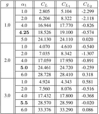
TABLE IV

LIFT COEFFICIENT OF FLOW OVER TWO CIRCULAR CYLINDERS AT FIXED

Re= 20, α2= 0.0ANDg= 1.0,2.0,3.0FOR1.0≤α1≤6.0

g α1 CL CL1 CL2

1.0

1.0 2.805 5.104 -2.299 2.0 6.204 8.322 -2.118 4.0 16.944 17.770 -0.826

4.25 18.526 19.100 -0.574 5.0 24.130 24.110 0.020

2.0

1.0 4.070 4.610 -0.540 2.0 7.035 8.342 -1.307 4.0 17.059 17.950 -0.891

5.0 24.461 24.720 -0.259 6.0 28.728 28.410 0.318

3.0

1.0 4.924 4.343 0.581 2.0 7.560 8.076 -0.516 4.0 17.432 17.800 -0.368

5.5 28.570 28.590 -0.020 6.0 33.376 33.290 0.086

III and IV. The drag coefficients of both cylinders decrease

with increasing α1, at fixed g, (see in the third column of

Table III). The lift coefficients of both cylinders increase

with increasingα1,at fixedg,as shown in the third column

of Table IV. We found that in the case of fixed Reynolds

number, Re = 20, rate of rotation corresponding to zero

drag force ( ˜α1) increases when g increases. For example,

Table III shows that atRe= 20, α˜1 corresponding to zero

drag force are α˜1 ≈4.25, (g = 1.0), α˜1≈5.0, (g= 2.0)

and α˜1 ≈ 5.5, (g = 3.0). The streamline patterns from

the simulations are shown in Fig.1- Fig.3 . The streamline patterns and pressure contours in the case rate of rotation

corresponding to zero drag force ( ˜α1)are occurred forg=

1.0,2.0,3.0 with respectively (see in Fig. 2).

In the second part, the left cylinder is rotating α2 = 1.0

and the right cylinder is rotating in counterclockwise angular

velocity. The effect of the rotation rate α1 is demonstrated

in Tables V and VI. The values of drag and lift coefficients

in the case of fixed Reynolds number,Re= 20and various

gap spacing, g = 1.0,2.0,3.0 for 1.0 ≤α1 ≤6.0 are also

shown. The drag coefficients of both cylinders decrease with

increasingα1,at fixedg, (see in the third column of Table V).

The lift coefficients of both cylinders increase with increasing

α1, at fixed g, as shown in the third column of Table VI.

The simulations of streamline patterns are shown in Fig.4 - Fig.6. This work is a fundamental problem which can be applied to some classes of obstructed flow.

V. CONCLUSION ANDSUGGESTION

Numerical results show the flow structure over two rotating circular cylinders with different radii depend on the rate of rotation, the gap spacing and the Reynolds number. We

found that at fixed gap spacingg,the drag coefficient of both

cylinders decrease with increasingαand the lift coefficient

of both cylinders increase with increasing α. In addition

we obtain the rate of rotation corresponding to zero drag

force ( ˜α1) increases when g increases at fixed Re = 20.

However these results ( ˜α1) are not the numerical solutions

of self-motion regime because its satisfy only CD ≈ 0

but CL is not close to zero. Numerical solutions of flow

−6 −4 −2 0 2 4

−4 −2 0 2 4 6 8

0.126 −0.236 −0.598 0.126

0.488

0.85

0.126 −1.68 −0.15

−0.1

0.3 0

−0.15

−0.3

−0.05 −0.3 −0.05 0.3

1

α=0.0 α=2.0

−6 −4 −2 0 2 4 −4

−2 0 2 4 6 8

−0.317 0.0214

0.36

1.38

0.0214 −0.656

−1.33 −0.656

−1.67

−0.994

−2.35

−1.67 1.38

−1.45 −0.1

−0.03

0.1

−0.03

α=0.0 α=2.0

−6 −4 −2 0 2 4

−4 −2 0 2 4 6 8 0.242

0.555

0.869 −0.0716

−0.0716 −1.01

−0.385 −2.27

−2.58

−1.95

−2.89

−1.95

−2.27

−1.64 0.242 −1.01 1.81

−3.21

−2.7 −0.025

0 −0.025

[image:3.595.87.253.89.279.2]

α=0.0 α=2.0

Fig. 1. streamline patterns of flow over two circular cylinders atRe= 20, g= 1.0,2.0,3.0andα1= 2.0, α2= 0.0.

TABLE V

DRAG COEFFICIENTS OF FLOW OVER TWO CIRCULAR CYLINDERS AT

g α1 CD CD1 CD2

1.0

1.0 9.886 3.037 6.849 2.0 6.958 1.343 5.615 4.0 2.902 -0.924 3.826 6.0 1.543 -0.324 1.867

2.0

1.0 8.528 2.344 6.184 2.0 6.376 0.888 5.488 4.0 2.106 -1.270 3.376 6.0 0.994 -0.510 1.504

3.0

1.0 8.632 2.623 6.009 2.0 7.432 1.482 5.950 4.0 4.410 0.066 4.344 6.0 1.565 -0.355 1.920

[image:3.595.350.501.579.736.2]

(4)

TABLE VI

LIFT COEFFICIENTS OF FLOW OVER TWO CIRCULAR CYLINDERS AT

g α1 CL CL1 CL2

1.0

1.0 5.988 5.974 0.014 2.0 9.965 10.360 -0.395 4.0 21.765 22.110 -0.345 6.0 39.713 39.010 0.703

2.0

1.0 7.218 4.774 2.444 2.0 10.396 8.795 1.601 4.0 21.040 19.660 1.380 6.0 37.257 35.780 1.477

3.0

1.0 10.069 4.677 5.392 2.0 13.600 8.959 4.641 4.0 24.659 20.570 4.089 6.0 39.565 36.430 3.135

−6 −4 −2 0 2 4

−4 −2 0 2 4 6 8

1.09 0.346 −0.0265

0.346

0.718

1.46

−0.0265 −0.771

−3 −0.399

−1.89

0 −0.01

−0.2

−0.1 −0.1

0.1

α = 0.0 α=4.25

-6 -4 -2 0 2 4 -4

-2 0 2 4 6 8

-2.28

-3.04

-6.08

-8.36

-3.04

-1.52 -0.76 -2.04

-0.5 -2.08

-2.12

-1.8 -1.6

-1.6 -2.12 -2

α=4.25 α=0.0

−6 −4 −2 0 2 4

−4 −2 0 2 4 6 8

1.37 0.306 −0.0479 −0.0479

−0.401

0.306

0.659

−0.0479 −0.401

−1.46 −1.81 −1.81

−0.01

0.1 −0.25

−0.01

α=5.0

α=0.0

-6 -4 -2 0 2 4 -4

-2 0 2 4 6 8

1.34

0.458

-11.1

0.458 0.458

1.67 1.69

1.64

1.6

1.88

2 1.88 1.67 1.6

1.5

α=0.0 α=5.0

−6 −4 −2 0 2 4

−4 −2 0 2 4 6 8

0.999 0.638 −0.0835 −0.445

−0.0835

0.277

0.638

−0.0835 −0.445

−1.89 −1.53

0 −0.021

−0.021 −0.15

α=0.0 α=5.5

-6 -4 -2 0 2 4 -4

-2 0 2 4 6 8

0.205

-0.814

-4.89

-1.83 0.205

0.205

0.5

0.6 0.7

0.74 0.76

0.8

0.78

0.74

1 0.85 0.76

0.76 0.4

α=5.5 α=0.0

Fig. 2. Streamline patterns and Pressure contours of flow over two circular cylinders at Re = 20, α˜1 = 4.25 (g = 1.0), α˜1 = 5.0 (g =

2.0), α˜1= 5.5 (g= 3.0)andα2= 0.0

have to transform to another coordinate system. In addition, numerical solutions of fluid flow over two rotating circular

cylinders for self-motion regime with different radii and in cases of higher Reynolds numbers may be investigated for future works.

−6 −4 −2 0 2 4

−4 −2 0 2 4 6 8

1.43 0.679 −0.0772 −0.455 −0.833 −1.21

−0.0772

0.301

0.679

1.06

1.43

1.81

0.301

−0.0772 −0.455

−1.59 0

−0.02

0.1

0.03

α=0.0 α=5.0

−6 −4 −2 0 2 4

−4 −2 0 2 4 6 8

2.06 2.06 0.0863

0.0863 −0.309

−1.1

−2.29

−1.5

0.0863

0.482

−0.309 −0.705

−1.5

−1.1 0

−0.12

0.03

α=0.0 α=6.0

−6 −4 −2 0 2 4

−4 −2 0 2 4 6 8

1.19 0.809 0.0567 −0.32

−1.07

−1.45 0.0567

0.433

0.809

−0.32 −0.696

−1.07 −1.82 0 −0.06

−0.15

−0.06

[image:4.595.379.476.107.533.2]

α=0.0 α=6.0

Fig. 3. streamline patterns of flow over two circular cylinders atRe= 20, α1= 5.0 (g= 1.0), α1= 6.0 (g= 2.0), α1 = 6.0 (g= 3.0)

andα2= 0.0

ACKNOWLEDGMENT

We would like to thanks the Faculty of Applied Science, King Mongkut’s University of Technology North Bangkok for supporting us in doing this work.

REFERENCES

[1] M. M. Zdravkovich, “Review of Flow Interference between Two Cir-cular Cylinders in Various Arrangements,”ASME J. Fluids Eng., vol. 99, pp. 618-633, 1977.

[2] S. Kang, “Characteristics of Flow over Two Circular Cylinders in a Side-by-Side Arrangement at Low Reynolds Numbers,”Phys. of Fluids, vol. 15, no. 9, pp. 486-498, 2003.

(5)

-6 -4 -2 0 2 4 -6

-4 -2 0 2 4 6 8

-1.53 -1.53

-1.76 -1.07

-1.3 -1.07

-0.837

-1.53 -1.76

-1.3 -0.146

-0.837

-1.07 -0.607 -0.607

-2.22 -0.837

-2.45

-0.376

-1.47

-0.8 -1.47

-1.47 -0.8

α=1.0 α=2.0

-6 -4 -2 0 2 4

-6 -4 -2 0 2 4 6 8

-2.72 -2.51 -2.3

-2.09

-2.72

-2.93

-2.51 -2.51

-1.88

-2.09 -0.2

-0.831

-1.04 -0.621

-0.2 -1.25

-2.3

-2.09 -1.04

-3.14 -2.6

-2.6 -2.6 -2.6

-2.6

-1.47

α=2.0 α=1.0

-6 -4 -2 0 2 4

-6 -4 -2 0 2 4 6 8

-4.5 -4.5 -4.74 -4.97

-0.237

-1.42

-3.79 -0.71

-0.947 -0.474

-1.89

-4.03 -3.79

-4.03 -4.26

-0.71 -4.26

-4.6 -4.38

-0.8

-4.38

-0.8 -4.6

-4.38 -4.6

[image:5.595.49.539.57.352.2]

α=1.0 α=2.0

-6 -5 -4 -3 -2 -1 0 1 2 3 4 -6

-4 -2 0 2 4 6 8

-0.799

-1.06

-1.31

-1.06

-0.0277

-0.0277 -0.799 -2.09

-1.57

-2.6

-1.83

-1.31 -0.799 -0.542 -0.799

-0.542 -1.57

-1.19

-1.47 -0.8 -1.19

α=1.0 α=4.0

-6 -4 -2 0 2 4

-6 -4 -2 0 2 4 6 8

-2.43 -2.91

-2.19

-1.94

-1.7 -0.243 -1.7

-0.972 -1.46

-1.21 -0.972

-2.43 -1.7

-3.16

-5.59 -2.3

-0.8 -0.8

α=4.0 α=1.0

-6 -4 -2 0 2 4

-6 -4 -2 0 2 4 6 8

-4.2

-3.92 -3.64

-3.36

-3.08 -0.28

-0.839

-1.12

-1.68

-3.36 -2.52

-3.08

-2.8 -0.839

-5.6 -3.78

-3.22

-0.94

-3.22

-3.22 α=4.0 α=1.0

[4] S. K. Panda, “Two-Dimensional Flow of Power-Law Fluids over a Pair of Cylinders in Side-by-Side Arrangement in the Laminar Regime,”

Braz. J. Chem. Eng., vol. 34, no. 2, pp. 507-530, 2017.

[5] S. Sungnul, “On the Representation of the Navier-Stokes Equations

-6 -4 -2 0 2 4

-6 -4 -2 0 2 4 6 8

-1.02 -1.35

0.618

-1.02 -0.0393

-1.68 -2.01

-3.65

-2.67 -4.31 -3.98

-0.696

-1.02 -1.35

-0.0393 -1.19

-1.19

-1.47

-0.8 -1.47

-0.8

α=1.0 α=6.0

-6 -4 -2 0 2 4

-6 -4 -2 0 2 4 6 8

-1.47 -0.111

-1.13

-1.47

-2.15

0.23 -1.13

-1.81 -3.17

-3.85 -2.83

-0.791 -2.34

-2.34 -0.8

α=6.0 α=1.0

-6 -4 -2 0 2 4

-6 -4 -2 0 2 4 6 8

-0.681

-0.341 -2.72

-2.72 -4.77

-1.02

-2.72 -1.02

-1.7 -2.38

-4.43 -4.09 -1.36

-5.11

-3.41 -2.5

-2.5 -1.2

-1.2

[image:5.595.50.284.395.688.2]

-2.5 α=6.0 α=1.0

in Cylindrical Bipolar Coordinate System,” in Proceedings in Annual National Symposium on Computational Science and Engineering 2005, pp. 340-348.

[6] S. J. Chorin, “Numerical Solution of the Navier-Stokes Equations,”

Math. Comp., vol. 22, pp. 745-762, 1968.

[7] D. B. Ingham and T. Tang, “A Numerical Investigation into the Steady Flow past a Rotating Circular Cylinder at Low and Intermediate Reynolds Numbers,” Journal of Computational Physics, vol. 87, pp. 91-107, 1990.

[8] D. Badr, S. C. R. Dennis and P. J. S. Young, “Steady and Unsteady Flow past a Rotating Cylinder at Low Reynolds Numbers,”Computer and Fluids, vol. 17, no. 4, pp. 579-609, 1989.