Sparse multi output radial basis function network construction using combined locally regularised orthogonal least square and D Optimality experimental design

Sparse Multi-Output Radial Basis Function Network Construction Using

Combined Locally Regularized Orthogonal Least Square and

D-Optimality Experimental Design

S. ChenÝ

, X. HongÞ

and C.J. HarrisÝ

Ý

Department of Electronics and Computer Science University of Southampton, Southampton SO17 1BJ, U.K.

Þ

Department of Cybernetics

University of Reading, Reading RG6 6AY, U.K.

Abstract

A new construction algorithm for multi-output radial basis function (RBF) network modelling is introduce by combining a locally regularized orthogonal least squares (LROLS) model selection with a D-optimality experimental design. The proposed algorithm aims to achieve maximized model robustness and sparsity via two effective and complementary approaches. The LROLS method alone is capable of producing a very parsimonious RBF network model with excellent generalization per-formance. The D-optimality design criterion further enhances the model efficiency and robustness. A further advantage of the combined approach is that the user only needs to specify a weighting for the D-optimality cost in the combined RBF model selecting criterion and the entire model construction procedure becomes automatic. The value of this weighting does not influence the model selection procedure critically and it can be chosen with ease from a wide range of values.

Keywords: Sparse modelling, orthogonal least squares, regularization, Bayesian learning, optimal experimental

design, D-optimality, radial basis function network, multi-output regression.

1

Introduction

The radial basis function (RBF) network has widely been studied [1]–[7]. For single-output nonlinear

data modelling or regression, the orthogonal least squares (OLS) algorithm [4],[8] provides an effective

means to construct parsimonious RBF networks with good generalization performance. The

parsimo-nious principle alone however is not entirely immune to over-fitting. If data are highly noisy, small

mod-els constructed may still fit into noise. A useful technique for overcoming over-fitting is regularization

[9]–[12]. From the Bayesian learning viewpoint, regularization is equivalent to adopting a

hyperparame-ter approach [13],[14], and a recent work [15],[16] has combined the OLS algorithm with an individually

regularized approach to derive an efficient single-output locally regularized OLS (LROLS) algorithm.

Optimal experimental designs [17] have been used to construct smooth model response surfaces based

design, model adequacy is evaluated by design criteria that are statistical measures of goodness of

exper-imental designs by virtue of design efficiency and experexper-imental effort. For regression models,

quantita-tively, model adequacy is measured as function of the eigenvalues of the design matrix. The D-optimality

design criterion [17] is most effective in optimizing the parameter efficiency and model robustness via

the maximization of the determinant of the design matrix. The traditional nonlinear model structure

determination based on optimal experimental designs is however inherent inefficient and

computation-ally prohibitive. Recently, effective model construction algorithms has been proposed for single-output

nonlinear modelling based on the computationally efficient OLS and LROLS algorithms, respectively,

coupled with the D-optimality experimental design [18],[19].

For the construction of multi-output RBF networks, one approach is to fit multiple single-output

models as, for example, in the work [20], and an alternative is to construct a single multi-output RBF

network model as, for example, in the work [21]. The latter approach has an advantage: a selected RBF

term must be significant in explaining all the outputs, and this can result in overall a smaller number

of regressors than the former approach to achieve the same modelling accuracy. Recent work [22] has

combine the local regularization approach with the multi-output OLS regression. This paper proposes

to combine the multi-output LROLS algorithm [22] with the D-optimality experimental design.

Compu-tational efficiency of the resulting algorithm is ensured by the orthogonal forward selection procedure.

The local regularization enforces model sparsity and avoids over-fitting while the D-optimality design

optimizes model efficiency and parameter robustness. The coupling effects of these two approaches in

the combined algorithm further enhance each other. The end result is an efficient yet simple algorithm for

constructing sparse multi-output RBF models that generalize well, especially under highly noisy learning

conditions. Moreover, the model construction process becomes fully automatic, and there is only one

user specified quantity which has no critical influence on the model selection procedure.

2

The multi-output radial basis function network

Consider the general discrete-time nonlinear system represented by the nonlinear model [23]:

(1)

where

(2)

and

are the system input and output vector variables with dimensions and

, respectively,

and are

positive integers representing the lags in and , respectively;

(4)

is the system white noise vector with covariance

and

being the

identity

matrix;

(5)

denotes the system “input” vector; and is the unknown

-dimensional system mapping.

The system model (1) is to be identified from an -sample observation data set

using some suitable functional which can approximate with arbitrary accuracy. One class of such

functionals is the RBF network model of the form:

(6)

for

, where

is the error between

and the-th model output

,

are the RBF

weights, the RBF kernels or regressors

(7)

are the RBF centers and

the positive width parameters. Typically, each training data

is

considered as a candidate RBF center, and the total number of candidate regressors in this case is

. Typical choices of nonlinearity are

thin-plate-spline

¾ ¾

Gaussian

½ ¾

multi-quadric

¾

¾

inverse multi-quadric

(8)

The multi-output RBF network model (6) can be written in a more concise form as

(9)

by defining

.. .

.. .

.. .

(10)

for , and

with

(12)

Further define

(13)

The RBF network model (6) is given in the matrix form as

(14)

Let an orthogonal decomposition of the regression matrixbe

(15)

where

. ..

.. . ..

. . .. ...  

(16)

and

(17)

which satisfies

, if . The RBF model (14) can alternatively be expressed as

(18)

where the orthogonal weight matrix

(19)

with

(20)

andsatisfies the triangular system

(21)

Knowingand, can readily be solved from (21).

3

The multi-output LROLS algorithm with D-optimality design

Before discussing this combined multi-output model construction algorithm, its two components, the

3.1 The LROLS algorithm

The multi-output LROLS algorithm is based on the following regularized error criterion [22]:

trace

(22)

where

is the regularization parameter vector, and the diagonal matrix

diag

. The original multi-output OLS algorithm [21] can be viewed as a special case

with

,. After some simplification, the criterion (22) can be expressed as [22]:

trace

trace

(23)

or

trace

(24)

Normalizing (23) by trace

yields

trace

trace

trace

(25)

Define the regularized error reduction ratio due to the regressor as

rerr

trace

(26)

Based on this ratio, significant regressors can be selected in a forward-regression procedure [22]. At the

-th stage, a regressor is chosen as the-th term of the subset model if it produces the largestrerr among

the remaining candidates, and the selection is terminated at the

-th stage when

rerr

(27)

is satisfied, where is a chosen tolerance. This produces a sparse model containing

significant regressors. The detailed algorithm selection procedure can be found in [22]. Notice that,

in the selection procedure, if

is too small (near zero), this term will not be selected. Thus, any

ill-conditioning or singular situations can automatically be avoided. The Bayesian evidence procedure

[13] can readily be extended to the multi-output case and thus used to “optimize” the regularization

parameters. This leads to the updating formulas for the regularization parameters (see [22]):

(28)

where

and

(30)

Usually a few iterations (typically 10 to 30) are sufficient to find an optimal.

It is worth emphasizing that, for this multi-output LROLS algorithm, the choice of is less critical

than the original OLS algorithm. This is because multiple regularizers enforce sparsity. If, for example,

is chosen too small, those unnecessarily selected terms will have a very large

associated with each

of them, effectively forcing their weights to zero [15],[16]. Nevertheless, an appropriate value for

is desired. Alternatively, the Akaike information criterion (AIC) [24],[25] can be adopted to terminate

the subset model selection process. The AIC can be viewed as a model structure regularization by

conditioning the model size using a penalty term to penalize large sized models. However, the use of

AIC or other information based criteria in forward regression only affects the stopping point of the model

selection, but does not penalizes the regressor that may cause poor model performance (e.g. too large

variance of parameter estimate or ill-posedness of the regression matrix), if it is selected. Or simply the

penalty term in AIC does not determine which regressor should be selected. Optimal experimental design

criteria offer better solutions as they are directly linked to model efficiency and parameter robustness.

3.2 The D-optimality experimental design

In experimental design, the data covariance matrix

is called the design matrix. The least squares

(LS) estimate of is given by

. Assume that (14) represents the true data

gener-ating process and

is nonsingular. Then, the estimate

is unbiased and the covariance matrix of

the estimate is determined by the design matrix:

Cov

(31)

It is well known that the model based on LS estimate tend to be unsatisfactory for an ill conditioned

regression matrix (or design matrix). The condition number of the design matrix is given by

(32)

with ,

, being the eigenvalues of

. Too large a condition number will result in unstable

LS parameter estimate while a small condition number improves model robustness. The D-optimality

design criterion maximizes the determinant of the design matrix for the constructed model. Specifically,

let be a column subset ofrepresenting a constructed

-term subset model. According to the

D-optimality criterion, the selected subset model is the one that maximizes

to prevent the selection of an oversized ill-posed model and the problem of high parameter estimate

variances. Thus, the D-optimality design is aimed to optimize model efficiency and parameter robustness.

The optimal experimental designs however do not provide means of parameter estimates and have to

rely on the LS or regularized LS methods for model parameter estimate. It is straightforward to verify that

maximizing

is identical to maximizing

or, equivalently, minimizing

[18]. Note that

(33)

and

(34)

By utilizing the additive property of (34) the D-optimality design criterion can be incorporated naturally

and efficiently with the orthogonal forward regression procedure.

3.3 The combined LROLS and D-optimality algorithm

The combined LROLS and D-optimality algorithm can be viewed as based on the combined criterion of

(35)

where is a fixed small positive weighting for the D-optimality cost. In this combined algorithm, the

updating of the model weights and regularization parameters is exactly as in the LROLS algorithm, but

the selection is according to the combined regularized error reduction ratio defined as

crerr

trace

(36)

and the selection is terminated with an

-term model when

crerr

for

(37)

The iterative RBF model selection procedure can now be summarized:

Initialization. Set ,

, to the same small positive value (e.g. 0.001), and choose a fixed.

Set iteration index .

Step 1. Given the current, select a subset model with

terms using the forward regression based

Step 2. Updateusing (28)–(30) with . If

remains sufficiently unchanged in two successive

iterations or a pre-set maximum iteration number is reached, stop; otherwise set and go

to Step 1.

The introduction of the D-optimality cost into the algorithm further enhances the efficiency and

robustness of the selected subset model and, as a consequence, the combined algorithm can often produce

sparser models with equally good generalization properties, compared with the LROLS algorithm. Note

that the model selection procedure is simplified and it is no longer necessary to specify the tolerance ,

as the algorithm automatically terminates when condition (37) is reached. Unlike the combined OLS and

D-optimality algorithm [18], the value of weighting does not critically influence the performance of

this combined LROLS and D-optimality algorithm andcan be chosen with ease from a large range of

values. This will be demonstrated in the following modelling examples. It should also be emphasized that

the computational complexity of this algorithm is not significantly more than that of the OLS algorithm.

This is simply because after the 1st iteration, which has a complexity of the OLS algorithm, the model set

contains only terms, and the complexity of the subsequent iteration decreases dramatically.

Typically, after a few iterations, the model set will converge to a constant size of very small . A

few more iterations will ensure the convergence of. Thus, this combined LROLS and D-optimality

design algorithm offers an efficient procedure to construct sparse multi-output RBF models with excellent

generalization performance without the need to apply costly cross-validation.

4

Nonlinear system modelling examples

Three examples were used to illustrate the effectiveness of the multi-output LROLS algorithm with the

D-optimality design and to compare it with the combined OLS algorithm and D-optimality design. The

RBF network model used in the simulation employed the thin-plate-spline nonlinearity.

Example 1. This was a simulated two-output time series process. The data set contained 1000 noisy

observations which were generated using the model

(38)

given the initial conditions

, where the zero-mean Gaussian

noise

had a covariance . The first 500 data samples were used for training

time series was governed by

(39)

Given the initial conditions

, the response of this

noise-free time series is depicted in Fig. 1. A two-output RBF network was used to model this time series, with

the input vector to the RBF network given by

(40)

As each training input was used as a candidate RBF center, the number of candidate regressors in the

RBF model (6) was .

For the multi-output modelling, the covariance of the modelling error ,

, is a

matrix. Typical scalar measures of modelling accuracy include trace

and .

Since is well-known to be a better measure of modelling accuracy, we will adopt the

following scalar measure

(41)

in our modelling comparison. Table 1 compares the values of

over the training and testing sets for

the RBF models constructed by the combined LROLS and D-optimality algorithm with those of the

combined OLS and D-optimality algorithm, given a wide range of values. Note that for this example

the true system noise had a

!!. It can be seen clearly that using the D-optimality

alone without regularization the constructed models can still fit into the noise unless the weighting is

set to some appropriate value. Combining regularization with D-optimality design, the results obtained

are consistent over a wide range ofvalues and, effectively, the value of has no serious influence on

the model construction process. The generalization capability of an identified model can best be tested

by examining the iterative model output. If the iterative model output can closely realize the behaviour

shown in Fig. 1, the identified model truly captures the underlying dynamics of the system and does

not simply fits the noise containing in the training data. Given the same initial conditions, the 49-term

RBF model identified by the combined LROLS and D-optimality algorithm with were used to

iteratively generate the network outputs

,, with the input

(42)

The iterative model outputs so generated are plotted in Fig. 2. It can be seen that the constructed RBF

Example 2. This was a simulated single-input two-output nonlinear system. The data were generated

using the model

(43)

where the system input was uniformly distributed in , and the system noises

were Gaussian with zero means and covariance . The data set contained 1000

samples, with the first 500 data points used for training and the last 500 data samples for model validation.

A two-output RBF network with the input

(44)

was employed to fit the noisy training data. The goodness of a fitted model was also evaluated by

computing the iterative model outputs with the input

(45)

For this example, the true system noise again had

!!. The modelling accuracies over

both the training and testing sets are compared in Table 2 for the two algorithms, the combined LROLS

and D-optimality and the combined OLS and D-optimality, with a range of values. Again it is seen

that, for the combined LROLS and D-optimality algorithm, the model construction process is insensitive

to the value of. The modelling accuracies in terms of Cov

for the two algorithms are

compared in Table 3, where Cov

denotes the covariance of the iterative model error. The

one-step predictions of the 35-term RBF model produced by the combined LROLS and D-optimality

algorithm withare illustrated in Fig. 3, and the iterative model outputs

generated by the

same RBF model are shown in Fig. 4.

Example 3. This example was a two-input two-output data set collected from a turbo-alternator

(Ap-pendix A11.3 in [26]). The data set contained 100 samples. The system inputs were the in-phase current

deviation and the out-of-phase current deviation

, and the system outputs were the voltage

deviation and the frequency deviation

. The two-output RBF network with the input vector

was used to fit this data set. As the data set was too short to be divided into a training set and a testing

set, the model validation in this case could only be performed by evaluating the iterative model outputs

,, with the input

(47)

over the training set of 100 samples. Table 4 compares the training accuracies of the two algorithms,

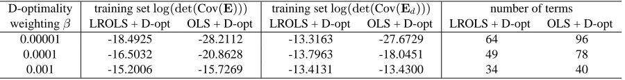
the combined LROLS and D-optimality and the combined OLS and D-optimality, given three values of

. Although there were no statistics over a testing data set to confirm the generalization capability of

a resulting model, it can be seen from Table 4 that the combined LROLS and D-optimality algorithm

performed more consistently with different values. Note that with , the two algorithms

had similar training accuracies, suggesting that the corresponding models should have similarly good

generalization capability. Figs. 5 and 6 depicted the model one-step predictions and the iterative model

outputs, respectively, over the training data for the 34-term RBF model constructed by the combined

LROLS and D-optimality algorithm with .

5

Conclusions

A locally regularized OLS algorithm with the D-optimality design has been proposed for constructing

sparse multi-output RBF network models. The efficiency of the subset model selection procedure is

ensured as usual with the orthogonal forward regression. By combining the two effective and

comple-mentary approaches for sparse and robust modelling, namely the local regularization and D-optimality

experimental design, the end result is an effective construction algorithm that is capable of producing

sparse multi-output RBF network models with excellent generalization performance. It has been shown

that the performance of the algorithm is insensitive to the D-optimality cost weighting, and the model

construction process is fully automated. The complexity of this combined model construction procedure

is only slightly more than that of the efficient OLS algorithm.

References

[1] M.J.D. Powell, “Radial basis functions for multivariable interpretation: a review,” in J.C. Mason and

M.G. Cox, Eds., Algorithms for Approximation. Oxford: Oxford University Press, 1987, pp.143–

[2] D.S. Broomhead and D. Lowe, “Multivariable functional interpolation and adaptive networks,”

Complex Systems, Vol.2, pp.321–355, 1988.

[3] J.E. Moody and C.J. Darken, “Fast learning in networks of locally tuned processing units,” Neural

Computation, Vol.1, No.2, pp.281–294, 1989.

[4] S. Chen, C.F.N. Cowan and P.M. Grant, “Orthogonal least squares learning algorithm for radial

basis function networks,” IEEE Trans. Neural Networks, Vol.2, No.2, pp.302–309, 1991.

[5] S. Chen, S.A. Billings and P.M. Grant, “Recursive hybrid algorithm for nonlinear systems

identifi-cation using radial basis function networks,” Int. J. Control, Vol.55, No.5, pp.1051–1070, 1992.

[6] M. Brown and C.J. Harris, Neurofuzzy Adaptive Modeling and Control. Englewood Cliffs, NJ:

Prentice-Hall, 1994.

[7] S. Chen, “Nonlinear time series modelling and prediction using Gaussian RBF networks with

en-hanced clustering and RLS learning,” Electronics Letters, Vol.31, No.2, pp.117–118, 1995.

[8] S. Chen, S.A. Billings and W. Luo, “Orthogonal least squares methods and their application to

non-linear system identification,” Int. J. Control, Vol.50, No.5, pp.1873–1896, 1989.

[9] A.E. Hoerl and R.W. Kennard, “Ridge regression: biased estimation for non-orthogonal problems,”

Technometrics, Vol.12, pp.55–67, 1970.

[10] C.M. Bishop, “Improving the generalisation properties of radial basis function neural networks,”

Neural Computation, Vol.3, No.4, pp.579–588, 1991.

[11] S. Chen, E.S. Chng and K. Alkadhimi, “Regularised orthogonal least squares algorithm for

con-structing radial basis function networks,” Int. J. Control, Vol.64, No.5, pp.829–837 1996.

[12] S. Chen, Y. Wu and B.L. Luk, “Combined genetic algorithm optimisation and regularised

orthogo-nal least squares learning for radial basis function networks,” IEEE Trans. Neural Networks, Vol.10,

No.5, pp.1239–1243, 1999.

[13] D.J.C. MacKay, “Bayesian interpolation,” Neural Computation, Vol.4, No.3, pp.415–447, 1992.

[14] M.E. Tipping, “Sparse Bayesian learning and the relevance vector machine,” J. Machine Learning

Research, Vol.1, pp.211–244, 2001.

[15] S. Chen, “Kernel-based data modelling using orthogonal least squares selection with local

regulari-sation,” in Proc. 7th Annual Chinese Automation and Computer Science Conf. in U.K. (Nottingham,

[16] S. Chen, “Locally regularised orthogonal least squares algorithm for the construction of sparse

kernel regression models,” in Proc. 6th Int. Conf. Signal Processing (Beijing, China), Aug.26-30,

2002, Vol.2, pp.1229–1232

[17] A.C. Atkinson and A.N. Donev, Optimum Experimental Designs. Oxford: Clarendon Press, 1992.

[18] X. Hong and C.J. Harris, “Nonlinear model structure design and construction using orthogonal least

squares and D-optimality design,” IEEE Trans. Neural Networks, Vol.13, No.5, pp.1245–1250,

2002.

[19] S. Chen, X. Hong and C.J. Harris, “Sparse kernel regression modelling using combined locally

regularized orthogonal least squares and D-optimality experimental design,” submitted to IEEE

Trans. Automatic Control, 2002.

[20] S.A. Billings, S. Chen and M.J. Korenberg, “Identification of MIMO non-linear systems using a

forward-regression orthogonal estimator,” Int. J. Control, Vol.49, pp.2157–2189, 1989.

[21] S. Chen, P.M. Grant and C.F.N. Cowan, “Orthogonal least squares algorithm for training

multi-output radial basis function networks,” IEE Proc. Part F, Vol.139, No.6, pp.378–384, 1992.

[22] S. Chen, “Multi-output regression using a locally regularised orthogonal least square algorithm,”

IEE Proceedings – Vision, Image and Signal Processing, Vol.149, No.4, pp.185–195, 2002.

[23] S. Chen and S.A. Billings, “Representation of non-linear systems: the NARMAX model,” Int. J.

Control, Vol.49, No.3, pp.1013–1032, 1989.

[24] H. Akaike, “A new look at the statistical model identification,” IEEE Trans. Automatic Control,

Vol.AC-19, pp.716–723, 1974.

[25] I.J. Leontaritis and S.A. Billings, “Model selection and validation methods for non-linear systems,”

Int. J. Control, Vol.45, No.1, pp.311–341, 1987.

[26] G.M. Jenkins and D.G. Watts, Spectral Analysis and Its Applications. San Francisco: Holden-Day,

Table 1: Comparison of modelling accuracy for the simulated two-output nonlinear time series modelling example. Cov : one-step prediction error covariance.

D-optimality training set Cov testing set Cov number of terms weighting¬ LROLS + D-opt OLS + D-opt LROLS + D-opt OLS + D-opt LROLS + D-opt OLS + D-opt

0.001 -6.78104 -18.1385 -6.07734 -5.32683 102 470

0.01 -6.68156 -10.1001 -6.08521 -5.39079 62 302

0.1 -6.55440 -6.87149 -6.09854 -5.95289 50 72

1.0 -6.43524 -6.51637 -6.03528 -6.04794 49 49

10.0 -6.38538 -6.43935 -6.12874 -6.10428 44 44

Table 2: Comparison of modelling accuracy for the simulated single-input two-output nonlinear system example. Cov : one-step prediction error covariance.

D-optimality training set Cov testing set Cov number of terms weighting¬ LROLS + D-opt OLS + D-opt LROLS + D-opt OLS + D-opt LROLS + D-opt OLS + D-opt

0.01 -6.59701 -10.8873 -6.10548 -5.41334 44 320

0.1 -6.56962 -6.84887 -6.07789 -5.95589 38 61

1.0 -6.49324 -6.56252 -6.13198 -6.08903 35 36

10.0 -6.50340 -6.55698 -6.11586 -6.06297 35 35

Table 3: Comparison of modelling accuracy for the simulated single-input two-output nonlinear system example. Cov

: model iterative error covariance over the entire 1000-sample data set.

D-optimality Cov number of terms

weighting¬ LROLS + D-opt OLS + D-opt LROLS + D-opt OLS + D-opt

0.01 -5.65089 -5.37460 44 320

0.1 -5.66776 -5.65160 38 61

1.0 -5.65614 -5.71936 35 36

10.0 -5.72100 -5.70334 35 35

Table 4: Comparison of modelling accuracy for the turbo-alternator modelling example. Cov :

one-step prediction error covariance, and Cov

: model iterative error covariance

D-optimality training set Cov training set Cov number of terms weighting¬ LROLS + D-opt OLS + D-opt LROLS + D-opt OLS + D-opt LROLS + D-opt OLS + D-opt

0.00001 -18.4925 -28.2112 -13.3163 -27.6729 64 96

0.0001 -16.5032 -20.8628 -13.7963 -18.0451 49 78

-1.5 -1 -0.5 0 0.5 1 1.5

-1.5 -1 -0.5 0 0.5 1 1.5

(a) -1.5 -1 -0.5 0 0.5 1 1.5

-1.5 -1 -0.5 0 0.5 1 1.5

(b)

Figure 1: Two dimensional representations of the noise-free time series observations: (a) phase plot of noise-free time series

, and (b) phase plot of noise-free time series

-1.5 -1 -0.5 0 0.5 1 1.5

-1.5 -1 -0.5 0 0.5 1 1.5

(a) -1.5 -1 -0.5 0 0.5 1 1.5

-1.5 -1 -0.5 0 0.5 1 1.5

(b)

Figure 2: Two dimensional representations of the iterative model outputs: (a) phase plot of iterative model output

, and (b) phase plot of iterative model output

. Initial conditions were

. The 49-term RBF model was constructed by the combined LROLS

-1.5 -1 -0.5 0 0.5 1 1.5

500 550 600 650 700

-1 -0.5 0 0.5 1

500 550 600 650 700

Figure 3: One-step prediction

superimposed on system output over the first 200 samples of

-1.5 -1 -0.5 0 0.5 1 1.5

500 550 600 650 700

-1 -0.5 0 0.5 1

500 550 600 650 700

Figure 4: Model iterative output

superimposed on system output over the first 200 samples

-2.6 -2.5 -2.4 -2.3 -2.2 -2.1 -2 -1.9 -1.8 -1.7

0 20 40 60 80 100

4.7 4.8 4.9 5 5.1 5.2 5.3

0 20 40 60 80 100

Figure 5: One-step prediction

superimposed on system output for the turbo-alternator

-2.6 -2.5 -2.4 -2.3 -2.2 -2.1 -2 -1.9 -1.8 -1.7

0 20 40 60 80 100

4.7 4.8 4.9 5 5.1 5.2 5.3

0 20 40 60 80 100

Figure 6: Model iterative output

superimposed on system output for the turbo-alternator