A Bayesian approach to modeling mortgage default and prepayment
Arnab Bhattacharyaa,1,∗, Simon P. Wilsona, Refik Soyerb
aDepartment of Statistics, School of Computer Science and Statistics, Trinity College, Dublin 02, Ireland. b
Department of Decision Sciences, The George Washington University, Washington, DC 20052, USA
Abstract
In this paper we present a Bayesian competing risk proportional hazards model to describe mort-gage defaults and prepayments. We develop Bayesian inference for the model using Markov chain Monte Carlo methods. Implementation of the model is illustrated using actual default/prepayment data and additional insights that can be obtained from the Bayesian analysis are discussed. Keywords: Reliability, proportional hazards model, competing risks, MCMC
1. Introduction and Overview
From a legal point of view mortgage default is defined as “transfer of the legal ownership of the property from the borrower to the lender either through the execution of foreclosure proceedings or the acceptance of a deed in lieu of foreclosure”; seeGilberto and Houston Jr. (1989). However, as noted byAmbrose and Capone(1998), it is common in the literature to define default as being delinquent in mortgage payment for ninety days.
As noted bySoyer and Xu(2010), due to major costs resulting from default to all involved par-ties, such as mortgage lenders, mortgagors, investors of mortgage backed securities (MBS) and the guarantors of MBS, assessment and management of the default risk is a major concern for financial institutions, and policy makers. As a result, there exists a rich literature on modeling mortgage default risk; see for example, Quercia and Stegman (1992) and Leece (2004). An important class of models is based on the ruthless default assumption which states that a rational borrower would maximize his/her wealth by defaulting on the mortgage if the market value of the mortgage exceeds the house value, and by prepaying if the market value of the house exceeds the book value of the house. Such models use an option theoretic approach and assume that the mortgage value and the prepayment and default options are determined by the stochastic behavior of variables such as property prices and the interest rates; see for example, Kau et al.(1990). Thus, under the option
∗
Corresponding author
Email addresses: [email protected](Arnab Bhattacharya),[email protected](Simon P. Wilson),
[email protected](Refik Soyer)
1This research was partly supported by Science Foundation Ireland (SFI) under Grant Number SFI/12/RC/2289
theoretic approach, other factors, such as the transaction costs, borrower characteristics, etc., are assumed to have no impact on values of the mortgage and the property underlined. The ruthless default assumption is not universally accepted in the literature and evidence against the validity of the assumption has been presented by many authors. Furthermore, as pointed out bySoyer and Xu (2010), implementation of this class of models requires availability of performance level data on individual loans over time which is typically difficult to obtain.
The alternate point of view, that does not subscribe to the ruthless default assumption, favors direct modeling of time to default of the mortgage. This approach involves hazard rate based models and also considers more direct determinants of mortgage default. This class of models includes competing risks and proportional hazards models ofLambrecht et al.(2003) and duration models ofLambrecht et al.(1997) that take into account individual borrower and loan characteristics. The competing risks models have been considered by many such asDeng et al.(1996);Deng and Order
(2000), Deng (1997), and Calhoun and Deng (2002). These can be considered as the competing risks versions of proportional hazards and multinomial logit models. The competing risks version of the PHM suggested byDeng(1997) involves evaluating hazard rates under the prepayment and default options. The author refers to these as prepayment and default risks. The competing risks approach is found to be useful in explaining the prepayment and default behaviors and improving the prediction of mortgage terminations. Application of these models to commercial mortgages can be found in Ciochetti et al.(2002) and in the more recent work byDeng and Haghani(2018). It is important to note that these class of models, focusing on assessment of time to default, differ from the classification type approaches that are typically used to assess whether a loan defaults or not. A recent review by Lessmann et al. (2015) discuss classification methods and algorithms that are used for credit scoring. An empirical comparison of classification algorithms for prediction of mortgage defaults can be found in Fitzpatrick and Mues (2016) where authors consider standard methods such as logistic regression as well as decision tree-based approaches such as random forests. Liu et al. (2015) note the potential limitations of classification models in dealing with censored data and propose hierarchical mixture models as an extension of the work ofTong et al. (2012).
Most of the above models use classical methods for estimation and as a result they do not provide probabilistic inferences. Some exceptions to these are the Bayesian work by Popova et al. (2008) who proposed Bayesian methods for forecasting mortgage prepayment rates,Soyer and Xu (2010) who considered Bayesian mixtures of proportional hazards models for describing time to default and
Kiefer(2010) who proposed an Bayesian approach for default estimation using expert information. More recently, Bayesian time series models have been considered in Aktekin et al.(2013) andLee et al. (2016). Bayesian mixture and segmentation models have been considered in Galloway et al.
has been considered bySun and Berger (1993) in reliability analysis and semiparametric Bayesian proportional hazards competing risk models have been introduced byGelfand and Mallick (1995) in survival analysis. Our work differ from these both in terms of the application and the specific approach taken. Furthermore, our focus is on time to default/prepayment since assessment of default time is important for financial institutions who offer loan modification and loss mitigation programs which are available in US as well as in Europe; seeOlrich (2006) andAndritzky (2014). In this paper we consider modeling duration of single-home mortgages. In doing so, we model default and prepayment probabilities simultaneously using competing risks proportional hazards models. We include both individual and aggregate level covariates in our model. We adopt the Bayesian viewpoint in the analysis and develop posterior and predictive inferences by using Markov chain Monte Carlo (MCMC) methods. In addition to providing a formalism to incorporate prior opinion into the analysis, the Bayesian approach enables us to describe all our inferences proba-bilistically and provides additional insights from the analysis. In what follows, we first introduce the competing risks proportional hazards models in Section 2. The Bayesian inference is presented in Section 3 where posterior and predictive analyses are developed. In Section 4 we illustrate implementation of our model and Bayesian methods using simulated data. Concluding remarks follow in Section 5.
2. Competing Risk Proportional Hazards Model
To introduce some notation let L denote the mortgage lifetime and TM denote the maturity
date of the mortgage loan. Note that if a mortgage loan is not defaulted or prepaid thenL=TM. If
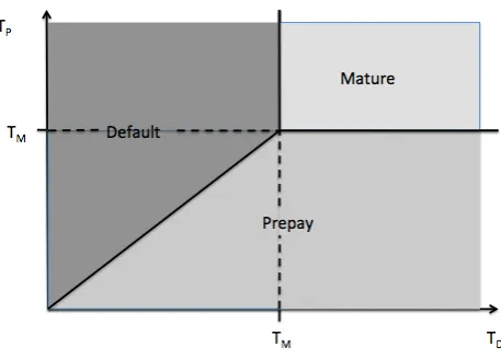
we letTD andTP denote time to default and time to prepayment for a mortgage loan, respectively, thenL=TM if (TD > TM) and (TP > TM). Figure1 illustrates the relationship betweenTM,TD
andTP. If bothTD andTP are larger thanTM then the mortgage will be paid on time. For a given mortgage loan it is of interest to infer events of “full payment”, default and prepayment. In other words, we are interested in computing probability statements such as P(TD > TM, TP > TM), P(TD < TP |TD < TM) orP(L > t|L < TM).
In view of the above, we can write
L=min(TD, TP, TM),
where bothTD andTP are random variables. We will modelTD andTP separately as proportional hazards models (PHMs) as inCox (1972). We denote the hazard (failure) rate for default and for prepayment as λD(t) and λP(t), respectively. We will refer to λD(t) as the default rate and to λP(t) as theprepayment rate. We model the default rate as
λD(t|XD(t)) =rD(t|ψD) exp(θD0 XD(t)), (1)
Figure 1: Competing risk representation of a mortgage that can default, prepay or mature at timeTM.
dependent covariates specific to default mortgages and θD is a vector of regression parameters. Similarly, the prepayment rate is modeled as
λP(t|XP(t)) =rP(t|ψP) exp(θP0 XP(t)). (2)
Note that for ease of notation, we use the same notation for all covariates, i.e.XD(t)≡XP(t)≡ X(t).
We assume that default and prepayment are “competing risks”, so that we only observe the first of them to occur. The observation of one at timetimplies that the other is right-censored at
t. We assume TD and TP to be independent, conditional on the baseline rate, parameters and set
of covariates. Thus, the joint survival function ofTD and TP is given by
P(TD > tD, TP > tP|rD(), rS(), θD, θP, X∗)
= P(TD > tD|rD(), θD, X∗)P(TP > tP|rS(), θP, X∗)
= exp
−
Z tD
0
λD(w)dw −
Z tP
0
λP(w)dw
,
whereX∗ ={X(w)|0≤w≤max(tD, tP)}. This standard assumption of conditional independence
of the time to each risk occurring means that, if the model parameter values were known in addition to the value of the covariates, then the occurrence of one of the risks does not change the distribution of the time to the other. This assumption allows for a considerable simplification in the computation of the inference procedure and yet does still permit some dependence between the times because they share common covariates.
Empirical evidence suggests that the default rate is non-monotonic. As discussed bySoyer and Xu(2010), it is reasonable to expect that the default rate is first increasing and then decreasing. A lifetime model having such hazard rate behavior is the lognormal model, other alternatives being generalised Gamma or log-logistic distribution which can also be entertained in our framework. Thus, we assume that baseline time to default TD follows a lognormal model with probability
density function
p(tD|µ, σ2) = √ 1
2πσ2tD exp
− 1
2σ2(log(tD)−µ) 2
, t >0.
Since it is not unreasonable to expect a similar behavior in the prepayment rate, we also assume that the baseline distribution of TP is also lognormal. Thus, the baseline model for TD will be
lognormal with parametersµD and σD2, and for prepayment with parametersµP and σP2.
The failure rate of the lognormal distribution can be written in terms of the standard Gaussian distribution function Φ. In fact the failure rates forTD and TP then take the form:
λD(t|XD(t)) = (2πσ
2 D)
−1/2t−1exp −0.5(log(t)−µD)2/σ2 D
1−Φ((log(t)−µD)/σD)
exp θ0DXD(t) (3)
and
λP(t|XP(t)) = (2πσ
2 P)
−1/2t−1exp −0.5(log(t)−µP)2/σ2 P
1−Φ((log(t)−µP)/σP)
exp θ0PXP(t); (4) see the Appendix for details on derivation of 3and 4.
3. Bayesian analysis of the competing risk PHM
We assume that data on N mortgages are available. From these, nD have defaulted, nP have
prepayed and nC =N −nD−nP are still active, including those that have matured successfully. TheN mortgages are indexedi= 1, . . . , nD for the defaulted mortgages,i=nD+ 1, . . . , nD+nP
for prepaid andi=nD+nP + 1, . . . , N for active. Let tD={tD1, . . . , tDnD}be the times of default and tP = {tPnD+1, . . . , t
P
nD+nP} be the times of prepayment. For the nC mortgages that are still active, let tC = {tCnD+nP+1, . . . , t
C
N} be the times since the initiation of mortgages; tCi =TM for
those that have matured.
Also observed are the covariates. Let Xi(t) = (Xi1(t), . . . , Xim(t)) be the vector of covariates for mortgageiat timet. Some of these are common covariates e.g. interest rates, while others are mortgage specific e.g. mortgage size or credit score. We assume that they are observed at a known set of times τ1 < τ2 <· · · < τm and that they are piecewise constant on intervals for which these times are the mid-points. Hence
Xi(t) =Xi(τj), sj−1 < t≤sj, (5)
let Xi ={Xi(τ1), . . . ,Xi(τm)} be the observed covariates for mortgage i and X = {Xi(τk)|i= 1, . . . , N;k= 1, . . . , m} be the set of all observed covariates. We would like to reiterate here that the set of covariates could be specific to mortgage type (default/prepay).
The unknown quantities in this model are the regression parametersθDandθP, and the baseline failure rate parameters ψ= (µD, σD2, µP, σP2). The required posterior distribution is therefore:
p(θD, θP, ψ|tD,tP,tC,X) ∝ p(tD,tP,tC|θD, θP, ψ,X)p(θD)p(θP)p(ψ). (6)
For the likelihood term P(tD,tP,tC|θD, θP, ψ,X), we assume observations are conditionally in-dependent, given the parameters. From the competing risks assumption, an observation tDi is an exact observation of TD and a right-censored observation ofTP; it is vice versa fortPi . Finally, tCi
is a right-censored observation of bothTD and TP. Hence:
p(tD,tP,tC|θD, θP, ψ,X)
=
nD
Y
i=1
p(tDi |θD,Xi)P(TP > tDi |θP,Xi)
!
×
nD+nP
Y
i=nD+1
p(tPi |θP,Xi)P(TD > tPi |θD,Xi)
×
N Y
i=nD+nP+1
P(TD > tCi |θD,Xi)P(TP > tCi |θP,Xi)
=
nD
Y
i=1
λD(tDi |Xi(tDi )) exp − Z tDi
0
λD(w|Xi(w)) +λP(w|Xi(w))dw !!
×
nD+nP
Y
i=nD+1
λP(tPi |Xi(tPi )) exp − Z tPi
0
λD(w|Xi(w)) +λP(w|Xi(w))dw !
×
N Y
i=nD+nP+1
exp −
Z tCi
0
λD(w|Xi(w)) +λP(w|Xi(w))dw !
(7)
where λD(t|Xi(t)) and λP(t|Xi(t)) are given by Equations 3 and 4, Xi(t) is given in Equation
5 and a formula for the integrals is given in Equation .4 of the Appendix. The formula for the integrals is more complex for time varying covariates, as noted in Cox and Oakes(1984).
An independent zero-mean normal prior is assumed for each component ofθD andθP, as well as
µD andµP. ForσD andσP, since no prior provides us with known full conditionals, an exponential
parameters where the priors and the posteriors are the same, the problem remains and can be solved using an improper prior (if it results in a proper posterior) or reducing dimension. We will see in the results that for the default model, identifiability is present. It is attributable to the low number of default mortgages under which parameter learning becomes very difficult; no such issue exists for the parameters under the prepaid model.
An MCMC procedure, based on the Metropolis within Gibb’s sampler (Tierney, 1994), has been implemented to sample fromp(θD, θP, ψ|tD,tP,tC,X). The covariate coefficient vectorsθD andθP are updated as blocks from their full conditional distributions with a Gaussian random walk
proposal, while each component ofψ is updated separately. The Appendix contains the details of the algorithm.
The MCMC output is a set of samples of all the unknowns from the posterior distribution. Let the number of samples be G, and let θD(g), θP(g) and ψ(g) denote the gth samples of ψ, θD and θP
respectively.
The MCMC output can be used to compute many quantities of interest. With the posterior samples, one can compute for a mortgage with a known set of covariates X = {X(w)|w ≥ 0}. The posterior predictive reliability function of the time to default is approximated by
P(TD > t|tD,tP,tC,X,X) ≈ 1
G G X
g=1
exp
−
Z t
0
λ(g)D (w)dw
, (8)
and the time to prepayment is approximated by
P(TP > t|tD,tP,tC,X,X) ≈ 1
G G X
g=1
exp
−
Z tP
0
λ(g)P (w)dw
, (9)
where λ(g)D (w) = r(g)D (w|ψ) exp(θD(g)0X(w)) and λ(g)P (w) = r(g)P (w|ψ) exp(θ(g)P 0X(w)), the values of r(g)D (w|ψ) and rP(g)(w|ψ) are given by Equation .1, using the parameter values in ψ(g), and a formula for the integrals is given by Equation .4of the Appendix.
that lie in their respective regions as defined in Figure1:
Defaults ⇔ tD < TM and tD < tP; Prepays ⇔ tP < TM and tP < tD;
Matures ⇔ tD ≥TM and tP ≥TM.
Since the marginal density is
f(t) =λ(t)R(t),
where λ(t) is failure rate and R(t) is reliability function as defined in equations 8 and 9, so the posterior density function forTD is approximated by
fD(t) ≈
1
G G X
g=1
λ(g)D (t) exp
−
Z t
0
λ(g)D (w)dw
.
A similar expression holds forfP(t).
4. The Freddie Mac Single Family Loan Dataset
The Federal Home Loan Mortgage Corporation (FHLMC), known as Freddie Mac, is a public company that is sponsored by the United States government. It was formed in 1970 to expand the secondary market for mortgages in the US. It has provided a dataset about single family loan-level credit performance data on a portion of fully amortizing fixed-rate mortgages that the company purchased or guaranteed. The dataset contains information about approximately 21.5 million fixed-rate mortgages that originated between January 1, 1999, and December 31, 2014. The dataset can be downloaded from the Freddie Mac website and is organised as two files for each quarter:
1. the origination data file that contains data concerning the set up of the loan;
2. the monthly performance data file that contains the monthly performance of each loan e.g. amount repaid, the outstanding principal, whether it is in default, etc.
There is also a smaller sample data set that contains a simple random sample of 50,000 loans selected from each year and a proportionate number of loans from subsequent years (the actual definition is 50,000 loans selected from each full vintage year and a proportionate number of loans from each partial vintage year of the full single family loan-level data set). The sample data set also has an origination and monthly performance file for each year
The data is highly unbalanced. This is well noted in the literature, with default rates typically staying around 1% to 2.5% for conventional mortgage loans whereas for subprime loans default rates rise over 14% in some years, see for exampleDanis and Pennington-Cross (2008).
4.1. Loan categorization
Four fields in the data were used to categorize each loan as default, prepay or active, and to define the observed time:
• zero_balance defines whether a particular loan’s balance has reduced to 0 or not, and has the following codes:
01 Prepaid or Matured (voluntary payoff);
03 Foreclosure Alternative Group (Short Sale, Third Party Sale, Charge Off or Note Sale); 06 Repurchase prior to Property Disposition;
09 REO Disposition; and empty Not Applicable.
• delinquency provides a value corresponding to the number of days the borrower has not paid the loan, according to the due date of last paid installment, or if a loan is acquired by REO, coded as:
0 Current, or less than 30 days past due; 1 30–59 days delinquent;
2 50–89 days delinquent; 3 90–119 days delinquent, etc.; R REO acquisition;
empty Unavailable.
• reporting_dateis the month that the observation is made in.
• months_remainis the number of months until the legal maturity of the loan.
Then the loan status was defined as:
• Prepaid if there exists a month where zero_balance = 01 AND repurchase = “N”. In this case, the prepaid timetP is the time from loan origination to thereporting_datewhere
this first happens.
• Activeif the loan could not be classified as Prepaid or Active AND the latestreporting_date corresponding to the loan is later than 01/01/2014 ANDzero_balanceis empty at that lat-est date ANDdelinquencyis not equal to R at that latest date. The active time is the time from loan origination to thereporting_datewhere this happens.
These definitions are not exhaustive; there are loans in the dataset that are discontinued without any clear information and such loans have been excluded from our analysis.
4.2. Covariates
The following covariates (fixed term) are available in the dataset: credit score, mortgage in-surance percentage (MI), number of units, combined loan-to-value (CLTV), debt-to-income (DTI), unpaid principal balance (UPB), original interest rate, number of borrowers, first homebuyer, occu-pancy status, property type, property state (state in which property resides) and current interest rate. Original interest rate refers to the rate at loan initiation while current interest rate con-tains monthly interest rates since loan start time. So the latter is the only variable whose values changes with time. Out of the rest, first homebuyer, occupancy status, property type and property state are categorical variables and have been converted to indicator variables. The covariate prop-erty state has been re-categorized into judicial or non-judicial state (renamed Foreclosure state), where in a judicial state, the lender needs to go through the court system for the foreclosure process. For the rest of the categorical variables, some of categories were of low frequency. For example, there are 6 categories in variable property_type, of which 81% were single family home and some categories like leasehold accounting for as low as 0.0003%. It was decided to group categories with extremely low frequencies for all the categorical variables. All the quanti-tative variables have been standardized. Furthermore strong correlation have been found between mortgage insurance percentageand combined loan-to-value, and between original and cur-rentinterest rates which led us to drop the latter in both the cases. Since current interest rate has been dropped we do not have to work with any time dependent covariate.
5. Analysis of the Data
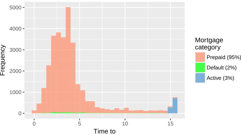
The data set comprised of 672208 mortgages originating in the year 1999. This data set is extremely unbalanced with 95% of the mortgages being prepaid, 3% being active and the only about 1.6% belonging to defaultcategory. This huge imbalance is evident in figure2.
Both θD and θP had Normal prior with zero mean and standard deviation 100. The mean
parameters µD and µP have zero mean Normal priors with standard deviation 10, while an expo-nential prior with mean 100 was assumed for the standard deviation parameters σD and σP. The starting value of each of the parameter chains were randomly selected using Normal and inverse gamma distributions for mean and standard deviation parameters respectively. The standard de-viation for the proposal distributions, for examples2
0 1000 2000 3000 4000 5000
0 5 10 15
Time to
Frequency
Mortgage category
Prepaid (95%)
Default (2%)
[image:11.595.95.495.113.338.2]Active (3%)
Figure 2: Histogram of time to default, prepaid and active times for each category.
from inverse gamma distributions to provide more diversity in the chains. The scale parameter (a) used in proposal forσD andσP was generated from uniform distribution.
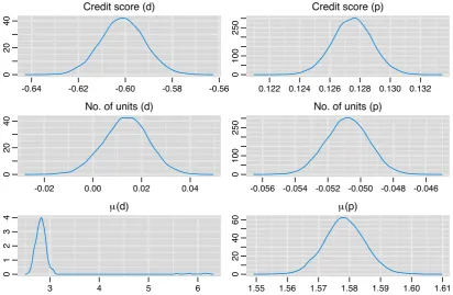
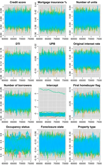
Rcpp (Eddelbuettel and Fran¸cois,2011) has been used to construct the MCMC algorithm. This has greatly improved the speed of the algorithm given that the data set is extremely large. The MCMC procedure was run in 50 chains for 75,000 iterations each. We set MCMC burn-in at 60000 and thinned the remaining by selecting every 50th sample. Trace plots, provided in the Appendix, for all the parameters show good mixing for all the covariates implying convergence. We provide the density plot constructed by combining the thinned chains for a subset of covariates in figure3. The skew in the density ofµD is caused by the slow convergence of a single chain. We assume that
this single chain suffers from slow convergence due to the problem of identifiability in proportional hazards models. The problem is further enhanced by the fact that the number of default mortgages is very low, hence making sufficient learning difficult.
Credit score (d)
-0.64 -0.62 -0.60 -0.58 -0.56
0
20
40
Credit score (p)
0.122 0.124 0.126 0.128 0.130 0.132
0
100
250
No. of units (d)
-0.02 0.00 0.02 0.04
0
20
40
No. of units (p)
-0.056 -0.054 -0.052 -0.050 -0.048 -0.046
0
100
250
μ(d)
3 4 5 6
0
1
2
3
4
μ(p)
1.55 1.56 1.57 1.58 1.59 1.60 1.61
0
20
40
[image:12.595.93.506.112.381.2]60
Figure 3: Density plot of combined samples from merging all the chains for credit score, number of units andµ, both for default (d) and prepaid (p) times. The long tail corresponding toµ(d) can be attributed to a single chain which is slow in converging.
insurance %both default and prepay rate increase, whereas for first time homebuyerboth the rates decrease. Also note that the estimated mean parameter (as also for the standard deviation parameter) of the baseline default rate is substantially greater than that of prepay.
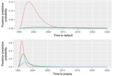
The posterior predictive densities for time to default (or prepay) corresponding to each mortgage can be computed using Equations8and 9(see discussion following these two equations). Figure4
shows predictive posterior distribution of time to default for 3 randomly chosen mortgages in the top panel. A similar plot corresponding to time to prepay has been provided in the lower panel. The posterior predictive densities for time to default are generally found to be flat, while those for prepay have variable shapes. Note that the area under the densities do not necessarily sum to 1 in these plots since we have truncated them at 2029, the maturity date of the mortgages.
Parameter Median 95% Prob. Interval
µD 2.817 (2.631, 3.077)
σD 0.963 (0.916, 1.028)
µP 1.578 (1.566, 1.591)
σP 0.717 (0.713, 0.721)
[image:12.595.188.402.628.697.2]Covariate Default Prepay
Median 95% Prob. Interval Mean 95% Prob. Interval
Credit score -0.601 (-0.620, -0.583) 0.128 (0.125, 0.130)
Mortgage insurance % 0.395 (0.376, 0.415) 0.068 (0.065, 0.070)
Number of units 0.014 (-0.005, 0.031) -0.051 (-0.053, -0.048)
Original DTI 0.124 (0.103, 0.146) 0.020 (0.018, 0.023)
UPB -0.069 (-0.093, -0.046) 0.305 (0.302, 0.307)
Original interest rate 0.412 (0.396, 0.429) 0.376 (0.374, 0.379)
No. of borrowers -0.296 (-0.316, -0.276) 0.055 (0.052, 0.058)
Intercept -3.090 (-3.356, -2.694) 0.182 (0.158, 0.207)
First time home-buyer -0.244 (-0.293, -0.194) -0.009 (-0.016, -0.003)
Occupancy status 0.460 (0.342, 0.575) 0.249 (0.237, 0.261)
Foreclosure state -0.110 (-0.149, -0.071) -0.080 (-0.085, -0.075)
Property type 0.304 (0.249, 0.362) -0.061 (-0.67, -0.054)
[image:13.595.100.495.376.641.2]*CovariateForeclosure state refers to whether the state is judicial or non-judicial.
Table 2: Summary of the marginal posterior distributions of θD and θP. The 95% probability intervals are the 2.5−97.5 percentiles of the sampled parameter values. Number of units under default mortgages is the only covariate that can be termed as not-significant, since the CI contain 0.
0.00 0.05 0.10 0.15
1999 2004 2009 2014 2019 2024 2029
Time to default
Posterior predictive
probability
0.0 0.2 0.4 0.6
1999 2004 2009 2014 2019 2024 2029
Time to prepay
Posterior predictive
probability
The mortgages and their covariate values are provided in table 3
6. Model Assessment
The suitability of the model is assessed by deriving, for each loan in the data:
• The probabilities that the loan defaults, prepays or remains active up to the end of the data, following the method in Section3, which can be compared to the actual outcome;
• If the mortgage defaulted then the predicted reliability function of the default time can also be computed from Equation 8, and hence the quantile of the observed time. A standardised residual can also be computed e.g. (tD −E(tD))/sd(tD), where tD is the observed default
time, E(tD) andsd(tD) are the mean and standard deviation of the posterior default time, derived from the predicted reliability function.
• Similarly, if the mortgage was prepaid then the predicted reliability function of the prepay time can be computed from Equation 9. The quantile of the observed prepay time and a standardised residual can be derived.
Active loans are right-censored observations of both the default and prepay times. The competing hazards model implies that default times are also right-censored observations of a prepay time, and vice versa.
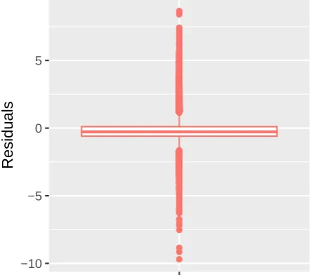
We assessed the fitted model on the sample data set in the year 1999, which has 30755 mort-gages. Figure5 shows a box plot of standardised residuals (as explained above) for all the default and the prepaid mortgages and is found to be centered around 0. If we isolate the defaulted mort-gages we find that the corresponding residuals are biased away from 0. Identifying mortmort-gages that defaulted is found to be difficult form that data we have since they constitute less than 2% of the whole set.
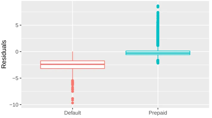
Separate box plots of standardised residuals for mortgages show a good fit for prepay, where residuals are slightly biased away from 0. However, for default mortgages almost all residuals are negative, which shows that the estimated mean time to default is higher than what was observed. We think that this can be largely attributed to huge contrast in proportion of each type of mortgages in the data set.
Covariate Default Prepay
Mortgage number 1 2 3 1 2 3
Credit score 724 541 750 787 668 619
Mortgage insurance % 12 30 0 0 0 30
Number of units 1 1 1 1 1 1
Original DTI 16 27 23 39 34 44
UPB 73000 112000 83000 37000 312000 204000
Original interest rate 6.875 10 8 6.875 7 9.625
No. of borrowers 2 2 2 1 2 2
First time home-buyer No No No No No No
Occupancy status Owner Owner Owner Owner Owner Owner
Foreclosure state Non-Jud Jud Non-Jud Non-Jud Non-Jud Non-Jud
[image:15.595.80.512.110.291.2]Property type SF SF SF SF SF SF
Table 3: The values of the covariates for the 6 mortgages that have been used for computing the posterior predictive densities in figure4 is provided here. Abbreviations used are: “Owner” - “Owner occupied”, “Non-Jud”/“Jud” -“Non-Judicial”/“Judicial” and “SF” - “Single family”.
● ● ● ● ● ● ● ● ● ● ● ● ● ● ● ● ● ● ● ● ● ● ● ● ● ● ● ● ● ● ● ● ● ● ● ● ● ● ● ● ● ● ● ● ● ● ● ● ● ● ● ● ● ● ● ● ● ● ● ● ● ● ● ● ● ● ● ● ● ● ● ● ● ● ● ● ● ● ● ● ● ● ● ● ● ● ● ● ● ● ● ● ● ● ● ● ● ● ● ● ● ● ● ● ● ● ● ● ● ● ● ● ● ● ● ● ● ● ● ● ● ● ● ● ● ● ● ● ● ● ● ● ● ● ● ● ● ● ● ● ● ● ● ● ● ● ● ● ● ● ● ● ● ● ● ● ● ● ● ● ● ● ● ● ● ● ● ● ● ● ● ● ● ● ● ● ● ● ● ● ● ● ● ● ● ● ● ● ● ● ● ● ● ● ● ● ● ● ● ● ● ● ● ● ● ● ● ● ● ● ● ● ● ● ● ● ● ● ● ● ● ● ● ● ● ● ● ● ● ● ● ● ● ● ● ● ● ● ● ● ● ● ● ● ● ● ● ● ● ● ● ● ● ● ● ● ● ● ● ● ● ● ● ● ● ● ● ● ● ● ● ● ● ● ● ● ● ● ● ● ● ● ● ● ● ● ● ● ● ● ● ● ● ● ● ● ● ● ● ● ● ● ● ● ● ● ● ● ● ● ● ● ● ● ● ● ● ● ● ● ● ● ● ● ● ● ● ● ● ● ● ● ● ● ● ● ● ● ● ● ● ● ● ● ● ● ● ● ● ● ● ● ● ● ● ● ● ● ● ● ● ● ● ● ● ● ● ● ● ● ● ● ● ● ● ● ● ● ● ● ● ● ● ● ● ● ● ● ● ● ● ● ● ● ● ● ● ● ● ● ● ● ● ● ● ● ● ● ● ● ● ● ● ● ● ● ● ● ● ● ● ● ● ● ● ● ● ● ● ● ● ● ● ● ● ● ● ● ● ● ● ● ● ● ● ● ● ● ● ● ● ● ● ● ● ● ● ● ● ● ● ● ● ● ● ● ● ● ● ● ● ● ● ● ● ● ● ● ● ● ● ● ● ● ● ● ● ● ● ● ● ● ● ● ● ● ● ● ● ● ● ● ● ● ● ● ● ● ● ● ● ● ● ● ● ● ● ● ● ● ● ● ● ● ● ● ● ● ● ● ● ● ● ● ● ● ● ● ● ● ● ● ● ● ● ● ● ● ● ● ● ● ● ● ● ● ● ● ● ● ● ● ● ● ● ● ● ● ● ● ● ● ● ● ● ● ● ● ● ● ● ● ● ● ● ● ● ● ● ● ● ● ● ● ● ● ● ● ● ● ● ● ● ● ● ● ● ● ● ● ● ● ● ● ● ● ● ● ● ● ● ● ● ● ● ● ● ● ● ● ● ● ● ● ● ● ● ● ● ● ● ● ● ● ● ● ● ● ● ● ● ● ● ● ● ● ● ● ● ● ● ● ● ● ● ● ● ● ● ● ● ● ● ● ● ● ● ● ● ● ● ● ● ● ● ● ● ● ● ● ● ● ● ● ● ● ● ● ● ● ● ● ● ● ● ● ● ● ● ● ● ● ● ● ● ● ● ● ● ● ● ● ● ● ● ● ● ● ● ● ● ● ● ● ● ● ● ● ● ● ● ● ● ● ● ● ● ● ● ● ● ● ● ● ● ● ● ● ● ● ● ● ● ● ● ● ● ● ● ● ● ● ● ● ● ● ● ● ● ● ● ● ● ● ● ● ● ● ● ● ● ● ● ● ● ● ● ● ● ● ● ● ● ● ● ● ● ● ● ● ● ● ● ● ● ● ● ● ● ● ● ● ● ● ● ● ● ● ● ● ● ● ● ● ● ● ● ● ● ● ● ● ● ● ● ● ● ● ● ● ● ● ● ● ● ● ● ● ● ● ● ● ● ● ● ● ● ● ● ● ● ● ● ● ● ● ● ● ● ● ● ● ● ● ● ● ● ● ● ● ● ● ● ● ● ● ● ● ● ● ● ● ● ● ● ● ● ● ● ● ● ● ● ● ● ● ● ● ● ● ● ● ● ● ● ● ● ● ● ● ● ● ● ● ● ● ● ● ● ● ● ● ● ● ● ● ● ● ● ● ● ● ● ● ● ● ● ● ● ● ● ● ● ● ● ● ● ● ● ● ● ● ● ● ● ● ● ● ● ● ● ● ● ● ● ● ● ● ● ● ● ● ● ● ● ● ● ● ● ● ● ● ● ● ● ● ● ● ● ● ● ● ● ● ● ● ● ● ● ● ● ● ● ● ● ● ● ● ● ● ● ● ● ● ● ● ● ● ● ● ● ● ● ● ● ● ● ● ● ● ● ● ● ● ● ● ● ● ● ● ● ● ● ● ● ● ● ● ● ● ● ● ● ● ● ● ● ● ● ● ● ● ● ● ● ● ● ● ● ● ● ● ● ● ● ● ● ● ● ● ● ● ● ● ● ● ● ● ● ● ● ● ● ● ● ● ● ● ● ● ● ● ● ● ● ● ● ● ● ● ● ● ● ● ● ● ● ● ● ● ● ● ● ● ● ● ● ● ● ● ● ● ● ● ● ● ● ● ● ● ● ● ● ● ● ● ● ● ● ● ● ● ● ● ● ● ● ● ● ● ● ● ● ● ● ● ● ● ● ● ● ● ● ● ● ● ● ● ● ● ● ● ● ● ● ● ● ● ● ● ● ● ● ● ● ● ● ● ● ● ● ● ● ● ● ● ● ● ● ● ● ● ● ● ● ● ● ● ● ● ● ● ● ● ● ● ● ● ● ● ● ● ● ● ● ● ● ● ● ● ● ● ● ● ● ● ● ● ● ● ● ● ● ● ● ● ● ● ● ● ● ● ● ● ● ● ● ● ● ● ● ● ● ● ● ● ● ● ● ● ● ● ● ● ● ● ● ● ● ● ● ● ● ● ● ● ● ● ● ● ● ● ● ● ● ● ● ● ● ● ● ● ● ● ● ● ● ● ● ● ● ● ● ● ● ● ● ● ● ● ● ● ● ● ● ● ● ● ● ● ● ● ● ● ● ● ● ● ● ● ● ● ● ● ● ● ● ● ● ● ● ● ● ● ● ● ● ● ● ● ● ● ● ● ● ● ● ● ● ● ● ● ● ● ● ● ● ● ● ● ● ● ● ● ● ● ● ● ● ● ● ● ● ● ● ● ● ● ● ● ● ● ● ● ● ● ● ● ● ● ● ● ● ● ● ● ● ● ● ● ● ● ● ● ● ● ● ● ● ● ● ● ● ● ● ● ● ● ● ● ● ● ● ● ● ● ● ● ● ● ● ● ● ● ● ● ● ● ● ● ● ● ● ● ● ● ● ● ● ● ● ● ● ● ● ● ● ● ● ● ● ● ● ● ● ● ● ● ● ● ● ● ● ● ● ● ● ● ● ● ● ● ● ● ● ● ● ● ● ● ● ● ● ● ● ● ● ● ● ● ● ● ● ● ● ● ● ● ● ● ● ● ● ● ● ● ● ● ● ● ● ● ● ● ● ● ● ● ● ● ● ● ● ● ● ● ● ● ● ● ● ● ● ● ● ● ● ● ● ● ● ● ● ● ● ● ● ● ● ● ● ● ● ● ● ● ● ● ● ● ● ● ● ● ● ● ● ● ● ● ● ● ● ● ● ● ● ● ● ● ● ● ● ● ● ● ● ● ● ● ● ● ● ● ● ● ● ● ● ● ● ● ● ● ● ● ● ● ● ● ● ● ● ● ● ● ● ● ● ● ● ● ● ● ● ● ● ● ● ● ● ● ● ● ● ● ● ● ● ● ● ● ● ● ● ● ● ● ● ● ● ● ● ● ● ● ● ● ● ● ● ● ● ● ● ● ● ● ● ● ● ● ● ● ● ● ● ● ● ● ● ● ● ● ● ● ● ● ● ● ● ● ● ● ● ● ● ● ● ● ● ● ● ● ● ● ● ● ● ● ● ● ● ● ● ● ● ● ● ● ● ● ● ● ● ● ● ● ● ● ● ● ● ● ● ● ● ● ● ● ● ● ● ● ● ● ● ● ● ● ● ● ● ● ● ● ● ● ● ● ● ● ● ● ● ● ● ● ● ● ● ● ● ● ● ● ● ● ● ● ● ● ● ● ● ● ● ● ● ● ● ● ● ● ● ● ● ● ● ● ● ● ● ● ● ● ● ● ● ● ● ● ● ● ● ● ● ● ● ● ● ● ● ● ● ● ● ● ● ● ● ● ● ● ● ● ● ● ● ● ● ● ● ● ● ● ● ● ● ● ● ● ● ● ● ● ● ● ● ● ● ● ● ● ● ● ● ● ● ● ● ● ● ● ● ● ● ● ● ● ● ● ● ● ● ● ● ● ● ● ● ● ● ● ● ● ● ● ● ● ● ● ● ● ● ● ● ● ● ● ● ● ● ● ● ● ● ● ● ● ● ● ● ● ● ● ● ● ● ● ● ● ● ● ● ● ● ● ● ● ● ● ● ● ● ● ● ● ● ● ● ● ● ● ● ● ● ● ● ● ● ● ● ● ● ● ● ● ● ● ● ● ● ● ● ● ● ● ● ● ● ● ● ● ● ● ● ● ● ● ● ● ● ● ● ● ● ● ● ● ● ● ● ● ● ● ● ● ● ● ● ● ● ● ● ● ● ● ● ● ● ● ● ● ● ● ● ● ● ● ● ● ● ● ● ● ● ● ● ● ● ● ● ● ● ● ● ● ● ● ● ● ● ● ● ● ● ● ● ● ● ● ● ● ● ● ● ● ● ● ● ● ● ● ● ● ● ● ● ● ● ● ● ● ● ● ● ● ● ● ● ● ● ● ● ● ● ● ● ● ● ● ● ● ● ● ● ● ● ● ● ● ● ● ● ● ● ● ● ● ● ● ● ● ● ● ● ● ● ● ● ● ● ● ● ● ● ● ● ● ● ● ● ● ● ● ● ● ● ● ● ● ● ● ● ● ● ● ● ● ● ● ● ● ● ● ● ● ● ● ● ● ● ● ● ● ● ● ● ● ● ● ● ● ● ● ● ● ● ● ● ● ● ● ● ● ● ● ● ● ● ● ● ● ● ● ● −10 −5 0 5 Residuals
Figure 5: Residuals of all the default and prepay mortgages combined. Note the slight bias below 0 which is caused by the default mortgages.
[image:15.595.187.410.355.551.2]● ● ● ● ● ● ● ● ● ● ● ● ● ● ● ● ● ● ● ● ● ● ● ● ● ● ● ● ● ● ● ● ● ● ● ● ● ● ● ● ● ● ● ● ● ● ● ● ● ● ● ● ● ● ● ● ● ● ● ● ● ● ● ● ● ● ● ● ● ● ● ● ● ● ● ● ● ● ● ● ● ● ● ● ● ● ● ● ● ● ● ● ● ● ● ● ● ● ● ● ● ● ● ● ● ● ● ● ● ● ● ● ● ● ● ● ● ● ● ● ● ● ● ● ● ● ● ● ● ● ● ● ● ● ● ● ● ● ● ● ● ● ● ● ● ● ● ● ● ● ● ● ● ● ● ● ● ● ● ● ● ● ● ● ● ● ● ● ● ● ● ● ● ● ● ● ● ● ● ● ● ● ● ● ● ● ● ● ● ● ● ● ● ● ● ● ● ● ● ● ● ● ● ● ● ● ● ● ● ● ● ● ● ● ● ● ● ● ● ● ● ● ● ● ● ● ● ● ● ● ● ● ● ● ● ● ● ● ● ● ● ● ● ● ● ● ● ● ● ● ● ● ● ● ● ● ● ● ● ● ● ● ● ● ● ● ● ● ● ● ● ● ● ● ● ● ● ● ● ● ● ● ● ● ● ● ● ● ● ● ● ● ● ● ● ● ● ● ● ● ● ● ● ● ● ● ● ● ● ● ● ● ● ● ● ● ● ● ● ● ● ● ● ● ● ● ● ● ● ● ● ● ● ● ● ● ● ● ● ● ● ● ● ● ● ● ● ● ● ● ● ● ● ● ● ● ● ● ● ● ● ● ● ● ● ● ● ● ● ● ● ● ● ● ● ● ● ● ● ● ● ● ● ● ● ● ● ● ● ● ● ● ● ● ● ● ● ● ● ● ● ● ● ● ● ● ● ● ● ● ● ● ● ● ● ● ● ● ● ● ● ● ● ● ● ● ● ● ● ● ● ● ● ● ● ● ● ● ● ● ● ● ● ● ● ● ● ● ● ● ● ● ● ● ● ● ● ● ● ● ● ● ● ● ● ● ● ● ● ● ● ● ● ● ● ● ● ● ● ● ● ● ● ● ● ● ● ● ● ● ● ● ● ● ● ● ● ● ● ● ● ● ● ● ● ● ● ● ● ● ● ● ● ● ● ● ● ● ● ● ● ● ● ● ● ● ● ● ● ● ● ● ● ● ● ● ● ● ● ● ● ● ● ● ● ● ● ● ● ● ● ● ● ● ● ● ● ● ● ● ● ● ● ● ● ● ● ● ● ● ● ● ● ● ● ● ● ● ● ● ● ● ● ● ● ● ● ● ● ● ● ● ● ● ● ● ● ● ● ● ● ● ● ● ● ● ● ● ● ● ● ● ● ● ● ● ● ● ● ● ● ● ● ● ● ● ● ● ● ● ● ● ● ● ● ● ● ● ● ● ● ● ● ● ● ● ● ● ● ● ● ● ● ● ● ● ● ● ● ● ● ● ● ● ● ● ● ● ● ● ● ● ● ● ● ● ● ● ● ● ● ● ● ● ● ● ● ● ● ● ● ● ● ● ● ● ● ● ● ● ● ● ● ● ● ● ● ● ● ● ● ● ● ● ● ● ● ● ● ● ● ● ● ● ● ● ● ● ● ● ● ● ● ● ● ● ● ● ● ● ● ● ● ● ● ● ● ● ● ● ● ● ● ● ● ● ● ● ● ● ● ● ● ● ● ● ● ● ● ● ● ● ● ● ● ● ● ● ● ● ● ● ● ● ● ● ● ● ● ● ● ● ● ● ● ● ● ● ● ● ● ● ● ● ● ● ● ● ● ● ● ● ● ● ● ● ● ● ● ● ● ● ● ● ● ● ● ● ● ● ● ● ● ● ● ● ● ● ● ● ● ● ● ● ● ● ● ● ● ● ● ● ● ● ● ● ● ● ● ● ● ● ● ● ● ● ● ● ● ● ● ● ● ● ● ● ● ● ● ● ● ● ● ● ● ● ● ● ● ● ● ● ● ● ● ● ● ● ● ● ● ● ● ● ● ● ● ● ● ● ● ● ● ● ● ● ● ● ● ● ● ● ● ● ● ● ● ● ● ● ● ● ● ● ● ● ● ● ● ● ● ● ● ● ● ● ● ● ● ● ● ● ● ● ● ● ● ● ● ● ● ● ● ● ● ● ● ● ● ● ● ● ● ● ● ● ● ● ● ● ● ● ● ● ● ● ● ● ● ● ● ● ● ● ● ● ● ● ● ● ● ● ● ● ● ● ● ● ● ● ● ● ● ● ● ● ● ● ● ● ● ● ● ● ● ● ● ● ● ● ● ● ● ● ● ● ● ● ● ● ● ● ● ● ● ● ● ● ● ● ● ● ● ● ● ● ● ● ● ● ● ● ● ● ● ● ● ● ● ● ● ● ● ● ● ● ● ● ● ● ● ● ● ● ● ● ● ● ● ● ● ● ● ● ● ● ● ● ● ● ● ● ● ● ● ● ● ● ● ● ● ● ● ● ● ● ● ● ● ● ● ● ● ● ● ● ● ● ● ● ● ● ● ● ● ● ● ● ● ● ● ● ● ● ● ● ● ● ● ● ● ● ● ● ● ● ● ● ● ● ● ● ● ● ● ● ● ● ● ● ● ● ● ● ● ● ● ● ● ● ● ● ● ● ● ● ● ● ● ● ● ● ● ● ● ● ● ● ● ● ● ● ● ● ● ● ● ● ● ● ● ● ● ● ● ● ● ● ● ● ● ● ● ● ● ● ● ● ● ● ● ● ● ● ● ● ● ● ● ● ● ● ● ● ● ● ● ● ● ● ● ● ● ● ● ● ● ● ● ● ● ● ● ● ● ● ● ● ● ● ● ● ● ● ● ● ● ● ● ● ● ● ● ● ● ● ● ● ● ● ● ● ● ● ● ● ● ● ● ● ● ● ● ● ● ● ● ● ● ● ● ● ● ● ● ● ● ● ● ● ● ● ● ● ● ● ● ● ● ● ● ● ● ● ● ● ● ● ● ● ● ● ● ● ● ● ● ● ● ● ● ● ● ● ● ● ● ● ● ● ● ● ● ● ● ● ● ● ● ● ● ● ● ● ● ● ● ● ● ● ● ● ● ● ● ● ● ● ● ● ● ● ● ● ● ● ● ● ● ● ● ● ● ● ● ● ● ● ● ● ● ● ● ● ● ● ● ● ● ● ● ● ● ● ● ● ● ● ● ● ● ● ● ● ● ● ● ● ● ● ● ● ● ● ● ● ● ● ● ● ● ● ● ● ● ● ● ● ● ● ● ● ● ● ● ● ● ● ● ● ● ● ● ● ● ● ● ● ● ● ● ● ● ● ● ● ● ● ● ● ● ● ● ● ● ● ● ● ● ● ● ● ● ● ● ● ● ● ● ● ● ● ● ● ● ● ● ● ● ● ● ● ● ● ● ● ● ● ● ● ● ● ● ● ● ● ● ● ● ● ● ● ● ● ● ● ● ● ● ● ● ● ● ● ● ● ● ● ● ● ● ● ● ● ● ● ● ● ● ● ● ● ● ● ● ● ● ● ● ● ● ● ● ● ● ● ● ● ● ● ● ● ● ● ● ● ● ● ● ● ● ● ● ● ● ● ● ● ● ● ● ● ● ● ● ● ● ● ● ● ● ● ● ● ● ● ● ● ● ● ● ● ● ● ● ● ● ● ● ● ● ● ● ● ● ● ● ● ● ● ● ● ● ● ● ● ● ● ● ● ● ● ● ● ● ● ● ● ● ● ● ● ● ● ● ● ● ● ● ● ● ● ● ● ● ● ● ● ● ● ● ● ● ● ● ● ● ● ● ● ● ● ● ● ● ● ● ● ● ● ● ● ● ● ● ● ● ● ● ● ● ● ● ● ● ● ● ● ● ● ● ● ● ● ● ● ● ● ● ● ● ● ● ● ● ● ● ● ● ● ● ● ● ● ● ● ● ● ● ● ● ● ● ● ● ● ● ● ● ● ● ● ● ● ● ● ● ● ● ● ● ● ● ● ● ● ● ● ● ● ● ● ● ● ● ● ● ● ● ● ● ● ● ● ● ● ● ● ● ● ● ● ● ● ● ● ● ● ● ● ● ● ● ● ● ● ● ● ● ● ● ● ● ● ● ● ● ● ● ● ● ● ● ● ● ● ● ● ● ● ● ● ● ● ● ● ● ● ● ● ● ● ● ● ● ● ● ● ● ● ● ● ● ● ● ● ● ● ● ● ● ● ● ● ● ● ● ● ● ● ● ● ● ● ● ● ● ● ● ● ● ● ● ● ● ● ● ● ● ● ● ● ● ● ● ● ● ● ● ● ● ● −10 −5 0 5 Default Prepaid Residuals
Figure 6: Separate box plots of residuals corresponding to default and prepay mortgages. The residuals for default mortgages show clear bias below 0.
The analysis suggests that we appear to be under-estimating the uncertainty in the default times. This can be explained by the imbalance in the data, with poor learning because of a much smaller number of observations of default, or by missing important covariates such as the location of the mortgaged property, local conditions and regulations as well as other borrower characteristics; see for example Goodman and Smith (2010). Also, as pointed out by a reviewer, the fact that default and prepayment behaviours are motivated by different factors may contribute to this. The model can possibly be improved by using behaviour specific covariates. As for this idea, while our method and logistic regression allows a different set of borrower covariates for default/prepay behaviour, RF provides a single unified set.
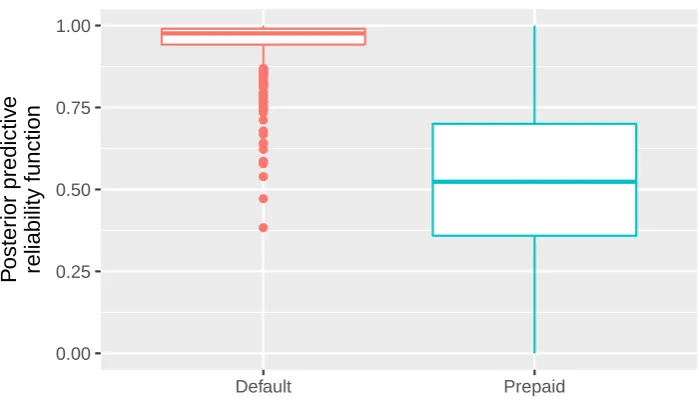
The contrast between default and prepaid mortgages is also evident when we calculated the predicted reliability function at the observed default or prepayment time. The median predicted reliability function for default mortgages is found to be 0.976 and (2.5,97.5) quantiles being (0.740,0.999), while those for prepaid are 0.524 (0.041,0.981). This confirms that in general the estimation of prepayment time performs well but that we over-estimate the default time. The box plots in figure 7 demonstrates the range of posterior reliability corresponding to both default and prepaid mortgages. Reliability is computed at the time to default or prepay.
7. Conclusion and future work
● ● ●
● ●
● ● ● ● ●
● ● ● ● ● ● ● ●
● ● ● ● ● ● ● ●
●
● ● ● ● ●
● ●
●
● ● ●
●
● ● ●
● ●
● ●
●
0.00 0.25 0.50 0.75 1.00
Default Prepaid
P
oster
ior predictiv
e
[image:17.595.123.473.112.314.2]reliability function
Figure 7: Box plots of posterior predictive reliability function computed for mortgages at time to default and prepay.
and vice versa; hence observation of one does contain information about the other that should be used in inference. Model inference can be done even for quite large data sets, as has been illustrated here for a set of single family loan data from Freddie Mac, where the relative effects of the different covariates on eventual prepayment or default have been quantified. Some difficulties with the inference were encountered, particularly for the defaults that were only a small percentage of the data. In particular, the identifiability issues with this model can cause some convergence issues with the MCMC implementation of the inference.
A natural extension of this work is to consider heterogeneity between mortgages, which would allow one to explore the between-mortgage variability and identify clusters of mortgages with similar properties. A random effects model is a simple way to allow for this e.g. the failure rates for mortgage iare now
λD,i(t, |XD,i(t)) =rD(t) exp(θTDXD,i(t) +φD,i) and λP,i(t, |XD,i(t)) =rP(t) exp(θTPXD,i(t) +φP,i),
whereφD,iandφP,i have a zero-mean prior distribution such as a Gaussian with variances that are
either known or are also specified by prior distributions. TheφD,iandφP,iquantify the differences
between default and prepay times from the average behaviour that is specified throughθD andθP. In terms of implementing inference for his model, the full conditional distributions ofθD and θP,
mortgage in the data set, with a resulting slowdown in the computation time.
8. References
Aktekin, T., Soyer, R. and Xu, F. (2013), ‘Assessment of mortgage default risk via Bayesian state space models’, The Annals of Applied Statistics7(3), 1450–1473.
Ambrose, B. W. and Capone, C. A. (1998), ‘Modeling the conditional probability of foreclosure in the context of single-family mortgage default resolutions’,Real Estate Economics26(3), 391–429.
Andritzky, J. R. (2014), ‘Resolving residential mortgage distress: Time to modify?’, IMF Working Paper, WP/14/226. Calhoun, C. A. and Deng, Y. (2002), ‘A dynamic analysis of fixed and adjustable-rate mortgage terminations’,The
Journal of Real Estate Finance and Economics24(1), 9–33.
Ciochetti, B. A., Deng, Y., Gao, Y. and Yao, R. (2002), ‘The termination of commercial mortgage contracts through prepayment and default: A proportional hazard approach with competing risks’,Real Estate Economics 30(4), 595–633.
Cox, D. R. (1972), ‘Regression models and life tables’,Journal of the Royal Statistical Society, Series B34(2), 187– 220.
Cox, D. R. and Oakes, D. (1984),Analysis of survival data, CRC Press.
Danis, M. A. and Pennington-Cross, A. (2008), ‘The delinquency of subprime mortgages’,Journal of Economics and Business60(1-2), 67–90.
Deng, R. and Haghani, S. (2018), ‘FHA Loans in foreclosure proceedings: Distinguishing sources of interdependence in competing risks’,Journal of Risk and Financial Management11(1), 1911–8074.
Deng, Y. (1997), ‘Mortgage termination: An empirical hazard model with a stochastic term structure’,The Journal of Real Estate Finance and Economics14(3), 309–331.
Deng, Y. and Order, R. V. (2000), ‘Mortgage terminations, heterogeneity and the exercise of mortgage options’, Econometrica68(2), 275–307.
Deng, Y., Quigley, J. M. and Order, R. V. (1996), ‘Mortgage default and low down payment loans: The costs of public subsidy’,Regional Science and Urban Economics26(3), 263–85.
Eddelbuettel, D. and Fran¸cois, R. (2011), ‘Rcpp: Seamless R and C++ integration’,Journal of Statistical Software 40(8), 1–18.
Fitzpatrick, T. and Mues, C. (2016), ‘An empirical comparison of classification algorithms for mortgage default prediction: evidence from a distressed mortgage market’,European Journal of Operational Research249(2), 427– 439.
Galloway, M., Johnson, A. and Shemyakin, A. (2017), ‘Time-to-default analysis of mortgage portfolios’, Model Assisted Statistics and Applications12(4), 359–367.
Gelfand, A. E. and Mallick, B. K. (1995), ‘Bayesian analysis of proportional hazards models built from monotone functions’,Biometrics51(3), 843–852.
Gilberto, S. M. and Houston Jr., A. L. (1989), ‘Relocation ppportunities and mortgage default’, Real Estate Eco-nomics17(1), 55–69.
Goodman, A. C. and Smith, B. C. (2010), ‘Residential mortgage default: Theory works and so does policy’,Journal of Housing Economics19(4), 280–294.
Kau, J. B., Keenan, D. C., III, W. J. M. and Epperson, J. F. (1990), ‘Pricing commercial mortgages and their mortgage-backed securities’,The Journal of Real Estate Finance and Economics3(4), 333–356.
Kiefer, N. M. (2010), ‘Default estimation and expert information’, Journal of Business and Economic Statistics 28(2), 320–328.
Lambrecht, B. M., Perraudin, W. R. M. and Satchell, S. (1997), ‘Time to default in the UK mortgage market’, Economic Modelling14(4), 485–499.
Lambrecht, B. M., Perraudin, W. R. M. and Satchell, S. (2003), ‘Mortgage default and possession under recourse: A competing hazards approach’,Journal of Money, Credit and Banking35(3), 425–442.
Lee, Y., R¨osch, D. and Scheule, H. (2016), ‘Accuracy of mortgage portfolio risk forecasts during financial crises’, European Journal of Operational Research249(2), 440–456.
Leece, D. (2004),Economics of the mortgage market: Perspectives on household decision making, Wiley-Blackwell. Lessmann, S., Baesens, B., Seow, H.-V. and Thomas, L. C. (2015), ‘Benchmarking state-of-the-art classification
algorithms for credit scoring: An update of research’,European Journal of Operational Research247(1), 124–136. Liu, F., Hua, Z. and Lim, A. (2015), ‘Identifying future defaulters: A hierarchical Bayesian method’, European
Journal of Operational Research241(1), 202–211.
Popova, I., Popova, E. and George, E. I. (2008), ‘Bayesian forecasting of prepayment rates for individual pools of mortgages’,Bayesian Analysis3(2), 393–426.
Quercia, R. G. and Stegman, M. A. (1992), ‘Residential mortgage default: A review of the literature’,Journal of Housing Research3(2), 341–379.
Soyer, R. and Xu, F. (2010), ‘Assessment of mortgage default risk via Bayesian reliability models’,Applied Stochastic Models in Business and Industry26(3), 308–330.
Sun, D. and Berger, J. O. (1993), Recent developments in Bayesian sequential reliability demonstration tests, in A. P. Basu, ed., ‘Advances in Reliability’, North-Holland, Amsterdam.
Tierney, L. (1994), ‘Markov chains for exploring posterior distributions’,The Annals of Statistics22(4), 1701–1728. Tong, E. N., Mues, C. and Thomas, L. C. (2012), ‘Mixture cure models in credit scoring: If and when borrowers
9. Appendix
Deriving the failure rate of the lognormal distribution
Let T be a lognormally distributed random variable with parameters µ and σ2 and density
function
f(t|µ, σ2) = √ 1
2πσ2texp
− 1
2σ2(log(t)−µ) 2
.
The failure rate is defined as
r(t) = f(t|µ, σ
2) P(T > t|µ, σ2) =
f(t|µ, σ2) R∞
t f(s|µ, σD)ds .
The lognormal failure rate can be calculated in terms of the normal cdf because T has the property that log(T) is normally distributed. Therefore
Z ∞
t
f(s|µ, σ2)ds= 1−P(T < t) = 1−P(log(T)<log(t)) = 1−Φ((log(t)−µ)/σ),
where Φ is the standard normal cdf. Hence
r(t) = (2πσ
2)−1/2t−1exp −0.5(log(t)−µ)2/σ2
1−Φ((log(t)−µ)/σ) . (.1)
Computing the integral of the failure rate function
The integral of the failure rate function appears in the likelihood function. It is assumed that the covariates X(t) vary piecewise constantly on intervals with mid-points τ1 < τ2 < · · · < τm.
So X(t) = X(τj) forsj−1 < t≤sj, with interval end-pointss0 = 0 and sj = 0.5(τj+τj+1), j =
1, . . . , m, withτm+1 =∞.
Let m0 = max{j|τj < tD}. The integral of the failure rate, needed in the specification of the
distribution of TD, is then:
Z tD
0
λD(w|XD(w))dw = m0 X
j=1
exp(θD0 XD(τj)) Z sj
sj−1
rD(w)dw+exp(θD0 XD(τj)) Z tD
sm0
rD(w)dw (.2)
The integral of the lognormal failure rate can be calculated in a closed form expression, using the fact that log(T) is Gaussian, and that
−log(P(T > t)) =
Z t
0
r(s)ds
holds for any failure rate, so that:
Z tb
ta
r(s)ds =
Z tb
0
r(s)ds−
Z ta
0
r(s)ds
= −log(P(T > tb)) + log(P(T > ta))
Substituting Equation .3into Equation .2gives:
Z tD
0
λD(w|XD(w))dw
=
m0 X
j=1
exp(θ0DXD(τj)) "
−log(1−Φ[(log(sj)−µD)/σD]) + log(1−Φ[(log(sj−1)−µD)/σD]) #
+ exp(θD0 XD(τm0)) "
−log(1−Φ[(log(tD)−µD)/σD]) + log(1−Φ[(log(sm0)−µD)/σD]) #
(.4)
The integral for TP, RtP
0 λP(w|XP(w))dw is also given by Equation .4 with tD, θD, µD and σD replaced bytP,θP, µP and σP respectively.
Details of the MCMC Algorithm for the Homogeneous Model
Sampling of the posterior distribution of Equation 6, with likelihood given by Equation 7, is done by a Metropolis within Gibbs algorithm. Each block of parameters are sampled from their full conditional distribution, with those samples obtained through a Metropolis proposal, as follows:
Sample θD. From a current valueθD, a random walk proposalθD∗ is made from a Gaussian with mean θD and variance s2θ,DIm×m, where Im×m is the identity matrix of dimension m and s2D is
tuned to provide a reasonable acceptance rate. The proposal is accepted with probability
min
1,p(tD,tP,tC|θ
∗
D, θP, ψ,X)p(θ
∗
D) p(tD,tP,tC|θD, θP, ψ,X)p(θD)
= min
1,p(θ
∗
D) QnD
i=1λ∗D(tDi |Xi(tDi )) p(θD)QnD
i=1λD(tDi |Xi(tDi ))
exp(−A∗−B∗−C∗) exp(−A−B−C)
,
where
A∗ =
nD
X
i=1 Z tDi
0
λ∗D(w|Xi(w))dw, B∗=
nD+nP
X
i=nD+1
Z tPi
0
λ∗D(w|Xi(w))dw and
C∗ =
N X
i=nD+nP+1
Z tCi
0
λ∗D(w|Xi(w))dw,
and,
A=
nD
X
i=1 Z tDi
0
λD(w|Xi(w))dw, B =
nD+nP
X
i=nD+1
Z tPi
0
λD(w|Xi(w))dw and
C=
N X
i=nD+nP+1
Z tCi
0
λ∗D(t|X(t)) is given by Equation3withθD =θ∗D,X(t) is given by Equation5andR0tλD(w|X(w))dw
is given by Equation.4.
Sample θP. This is identical to sampling from θD, with λD(t|X(t)) replaced by λP(t|X(t))
throughout.
Sample µD. From a current valueµD, a random walk proposalµ∗D is made from a Gaussian with
mean µD and variance s2µ,D, where s2µ,D is tuned to provide a reasonable acceptance rate. The proposal is accepted with probability
min
1,p(tD,tP,tC|θD, θP, ψ
∗,X)p(µ∗
D) p(tD,tP,tC|θD, θP, ψ,X)p(µD)
= min
1,p(µ
∗
D) QnD
i=1λ
∗
D(tDi |Xi(tDi )) p(µD) Qni=1D λD(tDi |Xi(tDi ))
× exp(−A
∗−B∗−C∗)
exp(−A−B−C)
,
whereA∗, B∗, C∗, A, BandChave already been defined earlier. ψ∗ = (µ∗D, σD2, µP, σP2),λ∗D(t|X(t)) is given by Equation3withµD =µ∗D,X(t) is given by Equation5and
Rt
0 λD(w|X(w))dwis given
by Equation.4.
Sample µP. This is identical to sampling from µD, with λD(t|X(t)) replaced by λP(t|X(t)) throughout andψ∗ = (µD, σ2D, µ∗P, σP2).
Sampleσ2D. From a current value σD2, a proposalσ2,D∗ is generated from a uniform distribution on the interval (aσ2D, σ2D/a), where a∈ (0,1) is tuned to provide a reasonable acceptance rate. The proposal is accepted with probability
min
(
1,p(tD,tP,tC|θD, θP, ψ
∗,X)p(σ∗,2
D )p(σD2 |σ 2,∗
D ) p(tD,tP,tC|θD, θP, ψ,X)p(σD2)p(σD2,∗|σD2)
)
= min
(
1,σ 2 Dp(σ
2,∗
D ) QnD
i=1λ∗D(tDi |Xi(tDi )) σ2,D∗p(σD2) QnD
i=1λD(tDi |Xi(tDi ))
× exp(−A
∗−B∗−C∗)
exp(−A−B−C)
) ,
where: ψ∗ = (µD, σD2,∗, µP, σP2),λ∗D(t|X(t)) is given by Equation3 with σD2 =σ 2,∗
D ,X(t) is given
by Equation5 and R0tλD(w|X(w))dw is given by Equation.4. Terms in the second multiplicand e.g.A∗, A, . . . etc have already been defined earlier.
Sample σP2. This is identical to sampling from σD2, with λD(t|X(t)) replaced by λP(t|X(t))
throughout andψ∗ = (µD, σ2D, µP, σP2,∗). MCMC output plots
to the twin problem of identifiability and low number of mortgages in this category. A larger proportion of default mortgages data and/or a longer run of the chain would have prevented this problem.
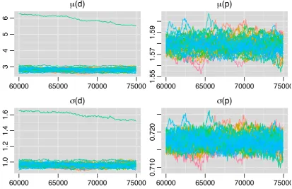
Trace plots of distributional parameters µd, µp, σd, σp are provided in .8. Note the single slow converging chain in the default category. The trace plots for all the variables for category default
μ(d)
60000 65000 70000 75000
3
4
5
6
μ(p)
60000 65000 70000 75000
1.55
1.57
1.59
σ(d)
60000 65000 70000 75000
1.0
1.2
1.4
1.6
σ(p)
60000 65000 70000 75000
0.710
[image:23.595.94.508.205.472.2]0.720
Figure .8: Trace plot of all distributional parameters. For parameters in default category, the single slow converging chain is visible here as well.
are provided in figure.9which seem to indicate towards fair convergence. The problem with a single chain is again noticeable in the intercept (βd0) trace. Trace plots of parameters associated with category prepaid are provided in figure.10. The traces converge well and seem to have identified the posteriors satisfactorily.
Machine learning output
The ML outputs - logistic regression+lasso and Random Forest are provided in this section.
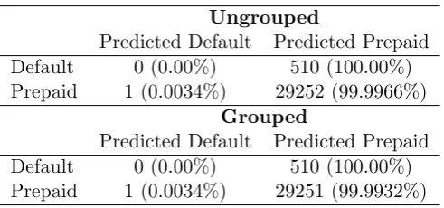
Ungrouped
Predicted Default Predicted Prepaid
Default 0 (0.00%) 510 (100.00%)
Prepaid 1 (0.0034%) 29252 (99.9966%)
Grouped
Predicted Default Predicted Prepaid
Default 0 (0.00%) 510 (100.00%)
[image:24.595.174.420.108.223.2]Prepaid 1 (0.0034%) 29251 (99.9932%)
Table .4: Confusion matrix of classification results for the test set, for both types of lasso penalties applied to logistic regression. Nearly all mortgages have been classified asPrepaid.
Random Forest. Table .5 is the confusion matrix for the random forest implementation to our data. Performance is much better that lasso, however default detection is lower than our model.
Predicted Default Predicted Prepaid
Default 143 (28.04%) 367 (71.96%)
Prepaid 0 (0.00%) 29253 (100.00%)
Credit score
60000 65000 70000 75000
-0.64
-0.62
-0.60
-0.58
Mortgage insurance %
60000 65000 70000 75000
0.36
0.38
0.40
0.42
0.44
Number of units
60000 65000 70000 75000
-0.02
0.00
0.02
0.04
DTI
60000 65000 70000 75000
0.08
0.10
0.12
0.14
0.16
UPB
60000 65000 70000 75000
-0.10
-0.06
-0.02
Original interest rate
60000 65000 70000 75000
0.38
0.40
0.42
0.44
Number of borrowers
60000 65000 70000 75000
-0.34
-0.32
-0.30
-0.28
-0.26
Intercept
60000 65000 70000 75000
-3
-2
-1
0
First homebuyer flag
60000 65000 70000 75000
-0.35
-0.25
-0.15
Occupancy status
60000 65000 70000 75000
0.3
0.4
0.5
0.6
Foreclosure state
60000 65000 70000 75000
-0.18
-0.14
-0.10
-0.06
Property type
60000 65000 70000 75000
0.20
0.25
0.30
0.35
[image:25.595.124.479.117.689.2]0.40
Credit score
60000 65000 70000 75000
0.122
0.126
0.130
Mortgage insurance %
60000 65000 70000 75000
0.064
0.068
0.072
Number of units
60000 65000 70000 75000
-0.056
-0.052
-0.048
DTI
60000 65000 70000 75000
0.016
0.020
0.024
UPB
60000 65000 70000 75000
0.300
0.304
0.308
Original interest rate
60000 65000 70000 75000
0.372
0.376
0.380
Number of borrowers
60000 65000 70000 75000
0.050
0.054
0.058
Intercept
60000 65000 70000 75000
0.14
0.18
0.22
First homebuyer flag
60000 65000 70000 75000
-0.020
-0.010
0.000
Occupancy status
60000 65000 70000 75000
0.23
0.25
0.27
Foreclosure state
60000 65000 70000 75000
-0.090
-0.080
-0.070
Property type
60000 65000 70000 75000
-0.070
-0.060
[image:26.595.123.479.124.697.2]-0.050