S Bandyopadhyay, D S Sharma and R Sangal. Proc. of the 14th Intl. Conference on Natural Language Processing, pages 23–32, Kolkata, India. December 2017. c2016 NLP Association of India (NLPAI)
Reference Scope Identification for Citances Using
Convolutional Neural Network
Saurav Jha MNNIT Allahabad, India
Aanchal Chaurasia NIT Rourkela, India
Akhilesh Sudhakar IIT (BHU), Varanasi, India
Anil Kumar Singh IIT (BHU), Varanasi, India
Abstract
In the task of summarization of a scientific paper, a lot of information stands to be gained about a refer-ence paper, from the papers that cite it. Automatically generating the ref-erence scope (the span of cited text) in a reference paper, corresponding to citances (sentences in the citing pa-pers that cite it) has great signifi-cance in preparing a structured sum-mary of the reference paper. We treat this task as a binary classi-fication problem, by extracting fea-ture vectors from pairs of citances and reference sentences. These fea-tures are lexical, corpus-based, sur-face and knowledge-based. We extend the current feature set employed for reference-citance pair identification in the current state-of-the-art system. Using these features, we present a novel classification approach for this task, that employs a deep Convolu-tional Neural Network along with two boosting ensemble algorithms. We outperform the existing state-of-the-art for distinguishing between cited spans and non-cited spans of text in the reference paper.
1 Introduction
Citation sentences or ‘citances’ that cite a reference paper (RP) can give valuable infor-mation about the larger context in which the RP is written, key ideas behind the RP and a concise synopsis of it. All of this is impor-tant for a task like scientific paper summa-rization, which not only requires the content of a paper but also meta-information about
it. This kind of information would otherwise have to be obtained from sources such as lit-erature reviews and surveys about the paper, which in turn is time-consuming and labor-intensive. This goal has also been outlined in a recent shared task on scientific paper summarization, the 3rd Computational
Lin-guistics Scientific Document Summarization Shared Task1.
The first step towards building a system that can obtain information about an RP from a citing paper (CP) that cites it, is to find spans of text in the RP that are cited by a particular citance in the CP. In the context of the above-mentioned shared task, this first step is referred to as Task 1A. Task 1A, thus offers a good foundation for the goal men-tioned above, by identifying the relevant ref-erence sentences for a citance. We present a novel approach to Task 1A. While we build on previous work by Yeh et al. (2017), our major contributions can be described as:
• We model a new feature set to rep-resent a citance-reference sentence pair along with building a classification sys-tem that uses a binary classification technique for classifying a <CP sen-tence, RP sentence> pair according to whether the CP sentence cites the RP sentence or not.
• We show performance gains over the results of Yeh et al. (2017)(which is the current state-of-the-art) by achiev-ing better F1-scores, usachiev-ing a feature set that has lesser number of features than that used in the above work.
• We explore various measures for evaluat-ing similarity between texts while
build-1http://wing.comp.nus.edu.sg/ cl-scisumm2017/
ing this feature set. Feature representa-tions extracted (as described later), are used to train three binary classifiers - an Adaptive Boosting Classifier (ABC), a Gradient Boosting Classifier (GBC) and a CNN classifier.
The datasets provided for this year’s as well as last year’s shared task have been used.
2 Related Work
There has been a large amount of work on the task of summarizing scientific docu-ments. However, as is clear from review sur-veys and papers such as Jones (2007), Teufel and Moens (2002) and Nenkova (2011), just using citances of a paper does not taken into account the context of a user or place the paper in a larger perspective of related work. Most of the related work on the task of iden-tifying text spans in the RP that correspond to a particular citance, have been presented at the shared task mentioned in the previ-ous section. We highlight some relevant work and various methods used for this task.
Yeh et al. (2017) also used a binary clas-sification approach for Task 1A, as we do. They used five classification algorithms to learn the binary classification model, with L2-SVM performing the best. Moraes et al. (2016) used SVM with subset tree ker-nel, a type of convolution kernel. They com-puted similarities between three tree repre-sentations of the citance and reference text. Li et al. (2016) used an SVM classifier with a topical lexicon to identify the best matching reference spans for a citance, using IFD simi-larity, Jaccard similarity and context similar-ity. The PolyU system by Cao et al. (2016), for Task 1a, used SVM-rank with lexical and document structural features to rank reference text sentences for every citance. Klampfl et al. (2016) applied a modified ver-sion of an unsupervised summarization tech-nique (TextSentenceRank) to the reference document. Nomoto (2016) treated the prob-lem as a ranking probprob-lem, learning one com-ponent of the similarity through a neural net-work and using TF-IDF scores for the other component. Aggarwal and Sharma (2016a) employed lexical and syntactic dependency cues in writing rules to extract text spans
in the RP for a given CP citance. Malen-fant and Lapalme (2016) presented a novel approach to solve this task. They first per-formed another task of identifying the facet of each sentence of the RP. These facets be-longed to a predefined set of facets, such as introduction, abstract, results, etc. They then used the facet information to match each sentence to a citance having the same facet in the CP.
3 Method
The structure of the dataset is described in Section 4.1. Citances and their actual refer-ence texts are extracted from gold-standard annotations. Citances in CPs are paired with each sentence in the RPs, along with a bi-nary label indicating their actual reference relations - 0 if the citance actually refers to the RP sentence and 1 if it doesn’t. For each such pair, a feature vector is extracted that describes the relatedness between the given citance and the reference sentence. These feature vectors, along with their correspond-ing labels, are used to train the binary clas-sifiers.
3.1 Feature Extraction
As mentioned in the section on related work, most approaches to this task have either been based on ranking of possible cited sentences in the RP for a given CP citance, or on binary classifying each RP sentence as rel-evant or irrelrel-evant to a given CP citance. We use the latter approach. Our method is based on the assumption that a CP sentence and corresponding RP sentence should be se-mantically and lexically similar, represent-ing similar meanrepresent-ing, idea or abstract con-cept. This is a natural assumption to make, since modeling the problem based on this assumption helps to separate relevant sen-tences (to the CP citance) in the RP from irrelevant ones. Inspired by the idea of Yeh et al. (2017), the feature set for each citance-reference pair is divided into three different
ferent from Yeh et al. (2017), when it comes to the set of features used. Through control experiments (Section 5.1), we show the effect of using our set of feature over theirs. We in-corporate several modified and newly added features.
The features marked by an asterisk (∗) are
the ones that are borrowed, but modified. The features marked by two asterisks (∗∗) are
the newly added features in this work. For features that have been borrowed from Yeh et al. (2017), more elaborate details about them can be seen in their work.
3.1.1 Lexical features
This class deals with the features represent-ing similarity measure of words for each pair of citance and reference sentence. As sug-gested by the results of Kenter et al. (2016) for short text similarity tasks, the overall sen-tence similarity measure based on each fea-ture is calculated by averaging the similari-ties over all the words in the sentences.
1. Word overlap∗: Word overlap between
the citance and the reference sentence based on five metrics: Dice coefficient, Jaccard coefficient, Cosine similarity, Levenshtein distance based fuzzy string similarity and modified gestalt pattern-matching based sequence matcher score, the last one as reported by Ratcliff and Metzener (1988).
2. TF-IDF similarity: The TF-IDF vec-tor cosine similarity between the ci-tance and the reference sentence as reported by Baeza-Yates and Ribeiro-Neto (2011).
3. ROUGE measure: The ROGUE (Lin and Hovy, 2003) metrics used are: ROGUE-1, ROGUE-2 and ROGUE-L.
4. Named entity overlap∗: Measured
using Dice coefficient, fuzzy string sim-ilarity, sequence matcher score and word2vec similarity.
5. Number overlap∗: Number overlap
between the citance and the reference sentence measured by fuzzy string simi-larity and sequence matcher score.
6. Significance of citation-related word pairs: The number of significant word pairs and the summation of significance scores of such word pairs extracted for each citance-reference pair based on Pointwise Mutual Information (PMI) score (Church and Hanks, 1989) collected from a dictionary containing significant words pairs appearing in the cited citance-reference pairs.
3.1.2 Knowledge-based features
1. WordNet-based semantic
similarity∗: The best semantic
similarity score between words in the citance and the reference sentence out of all the sets of cognitive synonyms
(synsets) present in the WordNet, following Miller (1992) and Pedersen et al. (2004).
3.1.3 Corpus-based feature
1. Word2Vec-based semantic
similarity∗∗: The word-to-word
semantic similarity between the ci-tance and the reference sentence is obtained based on the pre-trained embedding vectors of the GoogleNews corpus, following Mikolov et al. (2013). Campr and Jezek (2015) show several advantages that such embeddings of-fer, compared to those generated by traditional algorithms, such as LSA.
3.1.4 Surface features
This class includes features dealing primar-ily with the morphology of the reference sen-tences. These include:
1. Count of words: The count of words in the reference sentence.
2. Count of characters∗∗: The total
count of all characters in the reference sentence.
3. Count of numbers: The count of numbers in the reference sentence.
4. Count of special characters∗∗: The
number of special characters in the ref-erence sentence : “@”, “#”, “$”, “%”, “&”, “*”, “-”, “=”, “+”, “>”, “<”, “[”, “]”, “{”, “}”, “/”.
5. Normalized count of punctuation markers∗∗: The ratio of count of
punc-tuation characters to the total count of characters in the reference sentence.
6. Count of long words∗∗: The count of
words in the reference sentence exceed-ing six letters in length.
7. Average word Length∗∗: The ratio of
count of total characters in a word to the count of words in the reference sentence.
8. Count of named entities: The num-ber of named entities in the reference sentence.
9. Average sentiment score∗∗: The
overall positive and negative sentiment score of the reference sentence averaged over all the words, based on the Sen-tiWordNet 3.0 lexical resource as de-scribed by Baccianella et al. (2010).
10. Lexical richness∗∗: The lexical
rich-ness of the reference sentence based on Yule’s K index.
3.2 Classification Algorithms
As our approach treats the training data as pairs of citances and reference sentences, the number of reference sentences that a citance refers to is much smaller for a reference pa-per, leading to a highly imbalanced data set with the ratio of non-cited to cited pairs be-ing 383.83 : 1 in the combined corpus of de-velopment and training set and 355.76 : 1 in the test set corpus. This is not surprising since CPs usually cite only a small text span of an entire RP. Hence, our dataset is hugely imbalanced with negative examples being the majority. Following the work of Bowyer et al. (2002), we experimented with com-binations of three different degrees of Ran-dom under-sampling (20%, 30% and 35%) on the majority class (negative samples). On each undersampled dataset, we apply the SMOTE (Synthetic Minority Over-sampling Technique) method (Bowyer et al. (2002) ) to generate synthetic cited pairs until the ratio of the cited to non-cited pairs is 1:1. The best results were obtained with 30% ran-dom undersampling rate. To take care of
correlated features, if any, Principal Compo-nent Analysis (PCA), following Tipping and Bishop (1997) is applied on both training and testing feature sets. Experiments were done by varying the number of principal compo-nents from 30-40 and the best performance was obtained by retaining the top 35 princi-pal components.
For the classification task, we use two boosting ensemble algorithms: Adaptive Boosting Classifier (ABC) as described by Abe et al. (1999), Gradient Boosting Classi-fier (GBC) as described by Friedman (1999) and a deep Convolutional Neural Network (CNN) as described by Schmidhuber (2015). The implementation of ABC and GBC rely on sci-kit learn2, while the CNN is
imple-mented using Keras3 (Chollet et al. (2015)). Gensim (Rehurek and Sojka (2010)) is used to carry out word2vec related operations.
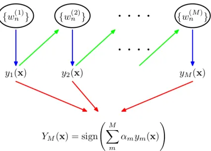
3.2.1 Boosting Ensemble Algorithms Boosting ensemble algorithms work by creating a sequence of models that attempt to correct the mistakes of the models used be-fore them in the sequence. Therebe-fore, these offer the added benefit of combining out-puts from weak learners (those whose perfor-mance is at least better than random chance) to create a strong learner with improved pre-diction performance, by paying higher focus on instances that have been misclassified or have higher errors by preceding weak rules. This is assisted by a majority vote of the weak learner’s predictions weighted by their individual accuracy. Figure 1 shows the il-lustration of such a boosting framework, as described by Bishop and Nasrabadi (2007).
The Adaptive Boosting Classifier (ABC)algorithm works in a similar way dis-cussed above. The base classifier (or weak learner) used in this case is a decision tree.
Gradient Boosting Classifier (GBC), on the other hand, begins by training sev-eral models sequentially on the original data set while allowing each model to gradually minimize the loss function of the whole sys-tem using the Gradient Descent method, as described by Collobert et al. (2004). The
2http://scikit-learn.org 3https://keras.io
Figure 1: Schematic illustration of the boost-ing framework. Adapted from Bishop and Nasrabadi (2007): each base classifier ym(x)
is trained on a weighted form of the train-ing set (blue arrows) in which the weights wn(m)depend on the performance of the
pre-vious base classifierym−1(x) (green arrows).
Once all base classifiers have been trained, they are combined to give the final classifier YM(x) (red arrows)
base classifiers in a GBC are regression trees. Since our task is a binary classification, only one regression tree is used as a special case.
3.2.2 Convolutional Neural Network Convolutional Neural Networks, as described in Schmidhuber (2015), have the ability to extract features of high-level abstraction with minimum pre-processing of data. They have been widely used for sentence classifica-tion problems, such as by Kim (2014). Re-cently, Ngoc Giang et al. (2016) also used CNNs for a sequence classification problem involving classification of DNA sequences by considering these sequences as text data. Given the success of CNNs on these, we ex-plore their use in our task.
However, in our case, a class-imbalance problem occurs due to the number of posi-tive reference-citance instances being far too low (495). These are too few examples for any deep learning model to extract mean-ingful features from the original text. Using the original sentences, and modeling it di-rectly as a sequence classification on pairs of sentences would introduce too much sparsity owing to this imbalance. Not surprisingly, our experiments on using original sentences
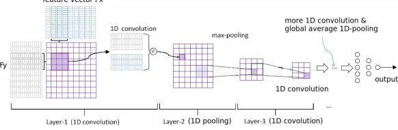
directly in an attention-based RNN model (2015) resulted in a precision score of 0.002 for positive and 0.24 for negative samples. Thus, we choose to train the CNN on the feature sets as inputs instead of the sentences directly. Figure 2 describes the CNN archi-tecture chosen by us after repeated experi-ments and tuning on the development data.
A 1D Convolutional layer accepts inputs of the form(Height * Width * Channels). In our case, we can visualize each feature vector as an image with a unit channel, unit height and a width equal to the number of features in the reduced feature vector obtained after applying PCA. Therefore, the input shape for the vector to be fed into the input layer of the CNN, becomes(No. of features * 1).
3.3 Post Filtering
The binary classifier may classify multiple sentences in the RP as positive, i.e., being relevant to a particular citance. However, the existence of inherent errors in the model means that all of these sentences may not be in the ideal text span of the RP corre-sponding to the citance. In order to reduce our false positive error rate, we post-process by filtering out some of these false positives. We use the approach of Yeh et al. (2017) for the post-filtering task. In this approach, the final output denotes the top-ksentences from the ordered sequence of classified refer-ence sentrefer-ences based on the TF-IDF vector cosine similarity score to measure the rele-vance between the citance and the reference sentences. All sentences other than the top-k are not included in the final output text span, even though the model might have labelled them as positive.
4 Experiments
4.1 Dataset
We use the development corpus, the training corpora and the test corpus provided for the CL-SciSumm Shared Tasks 20164 and 20175. As reported in Jaidka et al. (2016), each cor-pus comprises 10 reference articles, their cit-ing papers and annotation files for each refer-ence article. The citation annotations specify
4http://wing.comp.nus.edu.sg/cl-scisumm2016/ 5http://wing.comp.nus.edu.sg/ cl-scisumm2017/
Figure 2: Our CNN architecture: stack of two 1-D convolutional layers with 64 hidden units each (ReLu activations) + 1-D MaxPooling + stack of two 1-D convolutional layers with 128 hidden units each (ReLu activations) + 1-D Global Average Pooling + 50% Dropout + a single unit output dense layer (sigmoid activation)
citances, their associated reference text and the discourse facet that it represents.
4.2 Experimental Settings
Precision, Recall and F1-Score are used as evaluation metrics. The average score on all topics in the test corpus is reported. We run experiments on two separate training sets.
In the first run, we use data only from the 2016 shared task, and not from the 2017 shared task. This is because we need a com-mon ground for comparison with the existing state-of-the-art (Yeh et al. (2017)), which used this dataset. We first train our data on the training set, and tune the CNN’s hy-perparameters on the development set. We then augment the training data and the de-velopment data to train the final models. We test our model on the test provided as part of this dataset. Table 2 shows the perfor-mance of the CNN model on this test set, and compares it with the existing state-of-art and another well-performing model. We have reported only the CNN’s performance in this table as (as will be seen in the results of the second run), this is a better performing model than ABC and GBC, in our experi-mental setup.
In the second run, we make use of the datasets from both 2016 and 2017. Both the training datasets are augmented to form the initial training set. After tuning the CNN’s hyperparameters on the development set (which is the same for both 2016 and 2017), the initial training and development sets are augmented to form the final train-ing set. Grid search algorithm, as given by Bergstra and Bengio (2012), over 10-fold
cross validation is used to find the best model parameters for ABC and GBC listed in Ta-ble 1. Since the gold-standard annotations for the 2017 test set were not yet available at the time of conducting our experiments, we use only the test set of 2016. We report per-formance of ABC, GBC as well as the CNN classifier on this test set. Table 3 shows these results.
Table 1: Model parameter settings
Classifier Architecture and Param-eter settings
ABC
Learning rate for shrinking the contribution of each de-cision tree = 1.3, Boosting algorithm =SAMME.Rfor faster convergence
GBC
Learning rate for shrinking the contribution of regression tree = 0.15, Loss = De-viancefor probabilistic out-puts, No. of Boosting stages
=100
5 Results and Analysis
Precision, recall and F1-score obtained by the models on the test set with respect to the positive classes, evaluated by 10-fold cross validation are shown in Table 3. The CNN-based classifier was trained for 30 epochs. The best scores for each metric have been shown in bold.
Table 2: F1 scores of previous models
System
F1-scores
Yeh et al. (2017) 0.1443
Aggarwal and
Sharma (2016b) 0.11
Our Method 0.2462
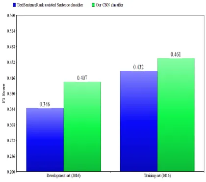
vious models used for the task. The L2-SVM system by Yeh et al. (2017) produced an F1-score of 0.1443, which is the highest reported yet to the best of our knowledge. Our model outperforms it in terms of F1-score. It must be mentioned here that Klampfl et al. (2016) reported an F1-score of 0.346 on the develop-ment set corpus and 0.432 on the training set corpus of 2016. However, we have not con-sidered their system in Table 2 because of the unavailability of their performance results on the test set corpus. Figure 3 compares the performance of our CNN classifier with their TextSentenceRank assisted sentence classi-fier on the development and training set cor-pus(80:20 train:test split)of 2016. Although the CNN classifier performs better on both the corpora, the improvement on the devel-opment corpus is much more significant than that on the training.
5.1 Control Studies
We run control studies to analyze the con-tribution of each class of features to our fi-nal performance. We also control for the different techniques used, such as SMOTE and PCA, to see their effect. These con-trol studies also help us to understand why our model outperformed the previous state-of-art. Since the CNN is our best performing classifier, we make use of it to perform these control studies.
[image:7.612.81.296.84.169.2]5.1.1 Effect of feature classes
Figure 4 shows the effect of each class of fea-tures. We obtain these graphs by removing one class of features each time from the fea-ture set and calculating the performance us-ing all the other classes. From the bar plot in Figure 4, it is apparent that the class of lexical features contributes the most in
dis-Figure 3: A comparison of the performance of our CNN-based classifier on the develop-ment and training set of 2016 with that of Klampfl et al. (2016)
Figure 4: F1 Scores of CNN Model with dif-ferent feature selection settings
pers. This class also has a high number of features, i.e., 10. Not using the class of sur-face features gives 0.0706 lesser F1-score than when using all the features. The plot also shows that the impact of WordNet-based fea-tures contribute the least to distinguishing between positive and negative examples.
It might therefore be concluded that part of the reason why our model outperforms the state-of-the-art is that their model does not make use of word2vec, while we do so. It also appears that the modified lexical features that we have used, namely, named entity overlap, number overlap and word overlap provide an added advantage to our model, over the state-of-the-art.
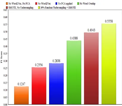
5.1.2 Effect of data-handling techniques
Figure 5 shows the contribution of differ-ent pre-processing and processing techniques used such as SMOTE (oversampling), under-sampling and dimensionality reduction us-ing PCA. There are a few observations that can be drawn from the bar plot in Figure 5. Firstly, dimensionality reduction is a crucial important step in this task. When PCA was not used on the feature set, the performance dropped from 0.5558 to 0.2838, which is a re-duction in F1-score of 0.2720. The existing
Figure 5: F1 Scores of CNN Model with dif-ferent feature selection settings
state-of-the-art has a higher number of fea-tures than our work does, and does not per-form dimensionality reduction on these fea-tures, which might be one of the reasons be-hind the better performance achieved in our work. Further, we see that oversampling us-ing SMOTE gives an improvement of 0.0555 and using undersampling over and above this further improves the performance by 0.0615.
Table 3: Results obtained by different models
Model Precision Recall
F1-score
ABC 0.7141 0.3579 0.4925
GBC 0.7439 0.3237 0.4512
CNN 0.6556 0.5973 0.5558
[image:8.612.90.293.59.233.2]false positives while a significant number of true positives have been missed out.
6 Future Work
To our knowledge, this is the first attempt which has used a deep learning model for addressing the task. However, for training our model, we had to be entirely dependent on the feature sets extracted. The num-ber of positive instances in the corpus pro-vided is still too low to train the model using the conventional CNN sequence-to-sequence approach, which, given more data, might be able to learn more interesting patterns in the citance-reference pairs. Also, recent extensions to word2vec such as the Para-graph Vector (Le and Mikolo (2014)) can be used to further enhance the semantic simi-larity measures between the reference-citance pairs.
Furthermore, the binary labels assigned to each <CP sentence, RP sentence> pair can be used to establish some partial order in be-tween the training instances, which in turn, can help in modeling the task as a Learning to rank problem. This ordering can then be incorporated to predict the relevance-based ranking of referenced sentences for a citance.
7 Conclusions
We describe our work on reference scope identification for citances using an extended feature set applied to three different classi-fiers. Among the classifiers trained to distin-guish cited and non-cited pairs, the CNN-based model gave the overall best results with an F1 score of 0.5558 on the combined corpus of CL-SciSumm 2016 and 2017. We also achieved an F1 score of 0.2462 on the 2016 dataset, which surpasses the previous state-of-the-art accuracy on the dataset. In addition to this, we carry out control studies reporting the contribution of various feature classes as well as feature selection methods that have been used by us.
References
Naoki Abe, Yoav Freund, and Robert E.
Schapire. 1999. A short introduction to boost-ing.
Peeyush Aggarwal and Richa Sharma. 2016a. Lexical and syntactic cues to identify reference scope of citance. InBIRNDL@ JCDL, pages 103–112.
Peeyush Aggarwal and Richa Sharma. 2016b. Lexical and syntactic cues to identify reference scope of citance. InBIRNDL@JCDL.
Stefano Baccianella, Andrea Esuli, and Fabrizio Sebastiani. 2010. Sentiwordnet 3.0: An en-hanced lexical resource for sentiment analysis and opinion mining. InLREC.
Ricardo A. Baeza-Yates and Berthier A. Ribeiro-Neto. 2011. Modern information retrieval - the concepts and technology behind search, second edition.
James Bergstra and Yoshua Bengio. 2012.
Random search for hyper-parameter optimiza-tion. Journal of Machine Learning Research, 13:281–305.
Christopher M. Bishop and Nasser M. Nasrabadi. 2007. Pattern recognition and machine learn-ing. J. Electronic Imaging, 16:049901.
Kevin W. Bowyer, Nitesh V. Chawla,
Lawrence O. Hall, and W. Philip Kegelmeyer.
2002. Smote: Synthetic minority
over-sampling technique. J. Artif. Intell. Res. (JAIR), 16:321–357.
Michal Campr and Karel Jezek. 2015. Compar-ing semantic models for evaluatCompar-ing automatic document summarization. InTSD.
Ziqiang Cao, Wenjie Li, and Dapeng Wu.
2016. Polyu at cl-scisumm 2016. In
BIRNDL@JCDL.
François Chollet et al. 2015. Keras. https: //github.com/fchollet/keras.
Ronan Collobert, Patrick Gallinari, Léon Bottou, Hélène Paugam-Moisy, Samy Bengio, and Yves Grandvalet. 2004. Large scale machine learn-ing.
Jerome H. Friedman. 1999. Greedy function ap-proximation: A gradient boosting machine.
Kokil Jaidka, Muthu Kumar Chandrasekaran,
Sajal Rustagi, and Min-Yen Kan. 2016.
Overview of the cl-scisumm 2016 shared task. InBIRNDL@JCDL.
Karen Spärck Jones. 2007. Automatic summaris-ing: The state of the art. Information Process-ing & Management, 43(6):1449–1481.
Tom Kenter, Alexey Borisov, and Maarten de
Ri-jke. 2016. Siamese cbow: Optimizing
word embeddings for sentence representations.
CoRR, abs/1606.04640.
Yoon Kim. 2014. Convolutional neural networks for sentence classification. InEMNLP.
Stefan Klampfl, Andi Rexha, and Roman Kern. 2016. Identifying referenced text in scientific publications by summarisation and classifica-tion techniques. InBIRNDL@JCDL.
Quoc V. Le and Tomas Mikolov. 2014. Dis-tributed representations of sentences and doc-uments. InICML.
Lei Li, Liyuan Mao, Yazhao Zhang, Junqi Chi, Taiwen Huang, Xiaoyue Cong, and Heng Peng. 2016. Cist system for cl-scisumm 2016 shared
task. InBIRNDL@JCDL.
Thang Luong, Hieu Pham, and Christopher D.
Manning. 2015. Effective approaches to
attention-based neural machine translation. In
EMNLP.
Bruno Malenfant and Guy Lapalme. 2016. Rali system description for cl-scisumm 2016 shared task. InBIRNDL@ JCDL, pages 146–155.
Tomas Mikolov, Ilya Sutskever, Kai Chen, Gre-gory S. Corrado, and Jeffrey Dean. 2013. Dis-tributed representations of words and phrases and their compositionality. InNIPS.
George A. Miller. 1992. Wordnet: A lexical database for english. Commun. ACM, 38:39– 41.
Luis Moraes, Shahryar Baki, Rakesh M. Verma, and Daniel Lee. 2016. University of houston at cl-scisumm 2016: Svms with tree kernels and sentence similarity. InBIRNDL@JCDL.
Ani Nenkova, Kathleen McKeown, et al. 2011. Automatic summarization. Foundations and Trends® in Information Retrieval, 5(2–3):103– 233.
Nguyen Ngoc Giang, Vu Anh Tran, Duc Luu Ngo, Dau Phan, Favorisen Lumbanraja, M Reza Faisal, Bahriddin Abapihi, Mamoru Kubo, and Kenji Satou. 2016. Dna sequence classification by convolutional neural network. 09:280–286, 01.
Tadashi Nomoto. 2016. Neal: A neurally en-hanced approach to linking citation and refer-ence. InBIRNDL@ JCDL, pages 168–174.
Ted Pedersen, Siddharth Patwardhan, and Jason Michelizzi. 2004. Wordnet: : Similarity - mea-suring the relatedness of concepts. InAAAI.
John W. Ratcliff and David Metzener. 1988.
Pattern Matching: The Gestalt Approach.
Radim Rehurek and Petr Sojka. 2010. Software framework for topic modelling with large cor-pora.
Jürgen Schmidhuber. 2015. Deep learning in neural networks: An overview. Neural net-works : the official journal of the International Neural Network Society, 61:85–117.
Simone Teufel and Marc Moens. 2002. Summa-rizing scientific articles: experiments with rel-evance and rhetorical status. Computational linguistics, 28(4):409–445.
Michael E. Tipping and Christopher M. Bishop. 1997. Probabilistic principal component anal-ysis.
Jen-Yuan Yeh, Tien-Yu Hsu, Cheng-Jung Tsai, and Pei-Cheng Cheng. 2017. Reference scope identification for citances by classification with text similarity measures. InICSCA ’17.