Visualization of Dynamic Reference Graphs
Ivan Rodin and Ekaterina Chernyak and Mikhail Dubov and Boris Mirkin National Research University Higher School of Economics
Moscow, Russia
Abstract
We present a tool for dynamic reference graph visualization. A reference graph is a graph based on key phrases retrieved from a time-indexed natural language text corpus. This tool may be useful for the analysis of con-nected pairs of latent topics, changes in the significance of these topics as well as in the relationship between them over various time periods.
1 Introduction
“Text visualization” is a rather ambiguous term. One of the approaches to text visualization is scene gen-eration, as described in (Chang et al., 2014). In our work, however, text visualization has a differ-ent meaning. Our interest lies in plotting meaning-ful elements from texts such as key phrases, named entities or terms. Retrieved plots may serve as a tool for information extraction and summarization. As shown in (Kucher and Kerren, 2015), there are many techniques for textual data analysis and visu-alization, and their number is rapidly growing.
In fact, the problem of text visualizaton can be di-vided into two subproblems: visualization of static and temporal textual data. The most known static text visualization technique is called “tag clouds” (Coupland, 1996). Many visualization techniques extend the idea of a tag cloud. For instance, in (Greene et al., 2015) key phrases are used to con-struct a concept lattice for a dataset of publica-tions. Lattice is visualized as an interactive tag cloud browser. In (Coppersmith and Erin, 2014), tags ex-tracted from tweets are colored according to the
po-litical preferences of tweet authors. Vennclouds, in-troduced in (Wang et al., 2012) present another ex-tention of tags clouds, comparing two texts by show-ing three tag clouds: one cloud containshow-ing tags from the first text, another one with tags from second text, and the third cloud showing words and phrases that appear in both texts.
Approaches based on tag cloud construction are also quite successful in the visualization of tempo-ral textual data. For example, the ThemeRiver vi-sualization tool, introduced in (Havre et al., 2000), shows thematic variations over time within a large collection of documents. In (Shahaf et al., 2013), tag clouds are placed inside graph nodes. The nodes are connected by an edge if they have a lot in com-mon, and are placed on the time axis as well.
Tag graphs are another extension of tag clouds. To construct a tag graph, one needs to introduce some sort of relation between tags. For example, in (Lloyd and D. Kechagias, 2005), the tags stand for named entities and one draws edges between tags that co-occur. (Berendt and Subasic, 2009) present a dynamic visualization technique for these tempo-ral co-occurence graphs.
In this paper, we suggest an approach to temporal textual data analysis which is based on dynamical reference graphs. The main difference of these ref-erence graphs from co-occurence graphs is that they are oriented. This allows to analyze how one term “refers” to another, as well as to retrieve more pat-terns describing the relations between terms. Our visualization also allows to analyze how the signifi-cance of certain terms changes over time.
2 Dynamic reference graph
To build a dynamic reference graph for a text collec-tion, one can use Algorithm 1.
Algorithm 1: Dynamic reference graph con-struction
Input :Time-indexed corpus of text documents and a list of key phrases.
Output:Dynamic reference graph.
1 Divide the corpus evenly intoTsequential time
periodsτ = 1..T.
2 Set a list ofNkey phrases (concepts)wi, i= 1..N. 3 forτ= 1..T do
4 Extract the information about static weighted
oriented reference graphGτthat should
include: 1) significance (the support value) of each concept in periodSτ(wi), which is the
number of documents where the concept appeared; 2) reference significance levels
Cτ(wi, wj),Cτ(wj, wi)for all pairs of
conceptswi, wj.
5 end
6 Define the lower threshold for support and
confidence levels. Draw a reference graphG1for τ= 1with respect to these thresholds.
7 forτ= 2..T do
8 Remove edges fromGτ−1are not inGτ 9 Remove nodes fromGτ−1are not inGτ 10 Add nodes fromGτthat are not inGτ−1 11 Add edges fromGτthat are not inGτ−1 12 end
Initial steps. The input to our system is a time-indexed corpus. The system divides documents into several time periods assuming that the number of documents in each time period is commensurable.
Next, we should define a list of concepts. They can be chosen just as the top frequent terms from the corpus. Sometimes it also makes sense to set the list of concepts manually. For example, if we want to analyze some specific topics from a corpus of news-paper articles, we can set a list of keywords to mon-itor and analyze, for example, only economical or technological news. This approach can be also use-ful in the analysis of the interaction between char-acters in fiction books where the concepts are just their names. Other possible approaches for term ex-traction are presented in (Siddiqi and Sharan, 2015) Building Gτ. Concepts define the nodes ofGτ. Weighted oriented edges of this graph are defined
by the co-occurrence of these concepts. We also re-trieve and store information about the significance of each concept in all time periods.
Support estimation. Let us define the signifi-cance of a conceptwiin time periodτ asSτ(wi) =
|Dτ(wi)|, whereDτ(wi)is a set of documents inτ where conceptwiappears more thanσtimes. By de-fault, we takeσ = 0, but in some cases that thresh-old may be increased.
Confidence estimation. Once we know the sup-port values for each conceptwiinτ, we can compute confidence values for the connections between pairs of concepts with non-zero support values. We say that conceptwi“refers” to conceptwjin time period
τ with confidenceCτ(wi, wj), whereCτ(wi, wj) =
|Dτ(wi)∩Dτ(wj)|
|Dτ(wi)| ∈[0; 1].
Having computed these confidence levels for con-nections between concepts in time periodτ, we can finally build a static oriented weighted graphGτ for that time period. An edge from conceptwi to con-ceptwjwith weightCτ(wi, wj)in this graph means thatwirefers towj with confidenceCτ(wi, wj). We can also specify the threshold for confidence which defines wheter or not edges should be displayed. Note that values ofCτ(wi, wj)close to1mean that ifwi occurs in a document, thenwj usually occurs as well. In other words, wj tends to occur in the context ofwi.
3 Datasets
Our test collection corresponds to the topic of newspaper analysis. We have collected a set of articles on economics from four Russian news-portals (“Izvestia”, “Kommersant”, “Moscow Kom-somoltes”, “Nezavisimaya gazeta”) that were pub-lished in 2014. This corpus (called “RuNeWC” – Russian Newspaper Web Corpus ) contains 4061 Russian language articles, divided into 26 time peri-ods. Every period has a length of 2 weeks.
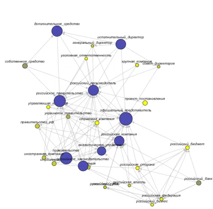
and 100 most frequent words. Finally, we manu-ally removed some concepts that are not semanti-cally important (ex.: “Kommersant reporter” [“Ko-rrespondent Kommersanta”] ). For graph visualiza-tion, we set the confidence threshold at 28 and sup-port threshold at 0.9. An example of dynamic graph visualisation for RuNeWC is presented in fig. 1.
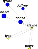
In order to provide an even more clear example, we created an English language corpus based on four books from a series of popular epic fantasy nov-els “A Song of Ice and Fire” (ASOIAF) written by George R. R. Martin. If we take the list of characters of that novel as an initial set of concepts the refer-ence graph then shows the co-occurrefer-ence of charac-ters in the book pages, typical cluscharac-ters of characcharac-ters, the significance of characters, as well as the change of these parameters over the time.
The plot in the first four books develops linearly: every next chapter describes actions that occurred after the actions of a previous one. To construct our corpus, we divided each chapter into several equal parts (2–7 parts, depending on the size of that chap-ter). Each part was then taken to the corpus as a single document. Then, the set of all documents was divided into groups of 50 sequential documents, forming 14 time periods. We didn’t take one chapter as a single time period, as the story of each chap-ter goes on behalf of one specific characchap-ter, and he automatically becomes the most important one. In constrast, the division of each chapter into several documents increased the precision of our support and confidence estimations for the concepts from the book.
In our experiment, we set the term frequency threshold σ = 1, i.e. considered a concept to be mentioned in a document if it appeared in that docu-ment two or more times. The threshold for the sup-port value was set at the level of 5, and minimum confidence value to 0.3.
As a result, we obtained a dynamic reference graph visualization that may serve as a schematic retelling of “Song of Ice and Fire” novel. Examples of dynamic graph visualisation for ASOIAF corpus are presented in figs. 2 to 41.
1Visualization video is available at
https://youtu.be/UaUGVPTdM-w.
[image:3.612.318.530.73.281.2]4 Visualization
Figure 1: RuNeWC reference graph at time periodτ = 9
(weeks 17-18 in 2014)
There are several tools for dynamic graph visual-ization, such as GraphStream2, KeyLines3, Gephi4.
For our task, we decided to use GraphStream as it is a well-documented Java Library which was specif-ically created for dynamic graphs editing and visu-alization. GraphStream is also effective in visual-ization of large graphs with thousands of nodes as it allows to create zoomable interface.
Our software tool can animate dynamic reference graphs based on their textual description. It ensures that the layout of a reference graphGτ for time pe-riodτ > 1depends on the layout ofGτ−1. It also
takes into account the information about the support of concepts: the greater the support, the bigger the corresponding node. The “age” of concepts (num-ber of periods where these concepts consecutively appear) is quite important as well: new nodes are marked with yellow, and when they become older, they gradually turn into blue. Moreover, if a con-cept appears for the first time (not after a break), the corresponding node receives a wide black border.
Our implementation comes with a graphical user interface. At any time step, the user can pause the animation process to explore the graph structure. All nodes of the input graph can be moved by simple
2http://graphstream-project.org/
Figure 2:This is dynamic graph at time periodτ = 11, which corresponds to the end of the third book. Color and border dif-ferentiation of nodes can show the age of concept in graph. For ex.: Oberyn is a character that appears for the first time, as cor-responding node is yellow with wide border, while “Tyrion” and other three nodes with deep blue colour have been presented in all periods from the very beginning.
drag and drop actions. Our software also handles node clicks: once a node is clicked, only those edges and nodes that are adjacent to it are displayed. More-over, the information about the support of the cor-responding concept during all time periods is dis-played in a separate window.
5 Future Work
Let us mention some future directions of our work: Integration. We are going to integrate our visu-alization software with a corpus browser that will allow users to generate and visualize their own cor-pora. To achieve that, we will have to build a unified system that will be responsible for both graph con-struction and visualization. The concept extraction system will be improved as well: it is possible to use the annotated suffix tree method (Dubov, 2015) for automatic concept extraction in case the user does not provide any.
[image:4.612.79.297.66.264.2]Analysis of connections. The system presented in this paper can be improved by adding support for contextual synonym extraction, as, for example, Petyr – Lord Baelish – Littlefinger in the ASOIAF
[image:4.612.390.464.234.330.2]Figure 3:The change of support for conceptRenlyduring the time periods.
Figure 4: As node of graph is clicked only nodes connected with chosen one are displayed.
corpus orRussian president – Vladimir Putinin the RuNeWC corpus. We will also compare presented mesure for confidence estimation with other simi-larity measures.
Graph analysis. Temporal cluster analysis can be particularly informative. Retrieving and highlight-ing of strongly connected components would allow users to detect some strong ongoing trends.
Graph layout. The layout of dynamic graphs still can be improved. In particular, we have to solve the problem of overlapping nodes that occasionally ap-pears in our software.
Acknowledgements
References
B. Berendt and I. Subasic. 2009. Stories in time: A graphbased interface for news tracking and discovery. In WI-IAT09.
A. X. Chang, M. Savva, and C. D Manning. 2014. Se-mantic parsing for text to 3d scene generation. In Proceedings of the ACL 2014 Workshop on Semantic Parsing.
G. Coppersmith and K. Erin. 2014. Dynamic Word-clouds and VennWord-clouds for Exploratory Data Analysis.
Association for Computational Linguistics. D. Coupland. 1996. Microserfs, Flamingo.
Mikhail Dubov. 2015. Text analysis with enhanced an-notated suffix trees: Algorithms and implementation. In Analysis of Images, Social Networks and Texts -4th International Conference, AIST 2015, Yekaterin-burg, Russia, April 9-11, 2015, Revised Selected Pa-pers, pages 308–319.
Gillian J Greene, Marcel Dunaiski, Bernd Fischer, Dmitry Ilvovsky, and Sergei O Kuznetsov. 2015. Browsing publication data using tag clouds over con-cept lattices constructed by key-phrase extraction. Susan Havre, Beth Hetzler, and Lucy Nowell. 2000.
ThemeRiver: Visualizing Theme Changes over Time.
Proceedings of the IEEE Symposium on Information Vizualization 2000.
A. Hulth. 2003. Improved automatic keyword extraction given more linguistic knowledge. The conference on Empirical methods in natural language processing. K. Kucher and A. Kerren. 2015. Text visualization
browser: A visual survey of text visualization tech-niques. Proceedings of IEEE Pacific Visualization Symposium (Visualization Notes), Englewood Cliffs, NJ.
L. Lloyd and S. Skiena D. Kechagias. 2005. Lydia: A system for large-scale news analysis, String Process-ing and Information Retrieval. Springer Berlin Hei-delberg.
O. A. Mitrofanova and V. P. Zaharov. 2009.
Automatic Analysis of Terminology in the Rus-sian Text Corpus on Corpus Linguistics [Av-tomatizirovannyy analiz terminologii v russkoy-azyichnom korpuse tekstov po korpusnoy lingvis-tike],. Dialog, available at: http://www.dialog-21.ru/digests/dialog2009/materials/.
Dafna Shahaf, Jaewon Yang, Caroline Suen, Heidi Wang Jeff Jacobs, and Jure Leskovec. 2013. Information cartography: creating zoomable, large-scale maps of information. Proceedings of the 19th ACM SIGKDD international conference on Knowledge discovery and data mining.
S. Siddiqi and A. Sharan. 2015. Keyword and keyphrase extraction techniques: A literature review. Interna-tional Journal of Computer Applications, 109(2).
H. Wang, D. Can, A. Kazemzadeh, F. Bar, and S. Narayanan. 2012.A system for realtime twitter sen-timent analysis of 2012 US presidential election cycle.