Data scarcity in modelling and simulation of a large scale WWTP : stop sign or a challenge

warwick.ac.uk/lib-publications Manuscript version: Author’s Accepted Manuscript

The version presented in WRAP is the author’s accepted manuscript and may differ from the published version or Version of Record.

Persistent WRAP URL:

http://wrap.warwick.ac.uk/116856

How to cite:

Please refer to published version for the most recent bibliographic citation information. If a published version is known of, the repository item page linked to above, will contain details on accessing it.

Copyright and reuse:

The Warwick Research Archive Portal (WRAP) makes this work by researchers of the University of Warwick available open access under the following conditions.

© 2019, Elsevier. Licensed under the Creative Commons Attribution-NonCommercial-NoDerivatives 4.0 International http://creativecommons.org/licenses/by-nc-nd/4.0/.

Publisher’s statement:

Please refer to the repository item page, publisher’s statement section, for further information.

1

Data Scarcity in Modelling and Simulation of a Large-scale WWTP: Stop sign or a

Challenge

Sina Borzooei

_{, Youri Amerlinck}

_{, Soroush Abolfathi}

_{, Deborah Panepinto}

_{, Ingmar}

Nopens

_{, Eugenio Lorenzi}

_{, Lorenza Meucci}

_{, Maria Chiara Zanetti}

1. Department of Environment, land and infrastructure Engineering (DIATI), Politecnico di

Torino, Torino, Italy.

2. Department of Data Analysis and Mathematical Modelling, Faculty of Bioscience

Engineering, Ghent University, Ghent, Belgium.

3. Warwick Water Research Group, School of Engineering, The University of Warwick

Coventry, UK.

4. Società Metropolitana Acque Torino S.p.A. Corso XI Febbraio 14, 10152, Torino (TO),

Italy

*Corresponding author: [email protected]

This is the pre-print version of manuscript. The post-print version can be found online:

https://doi.org/10.1016/j.jwpe.2018.12.010

2

Abstract

Data scarcity can be considered as the main limitation for a more widespread utilization of mathematical

models in the design, optimization and control of biological nutrient removal activated sludge systems

(BNRAS). High cost and demanding workload related to experimental data and sufficient sampling

campaigns make the data collection process an unpleasant necessity for managing stakeholders in

modelling projects. Complicated use of online-sensors leading to frequent erroneous readings and

dynamic nature of wastewater treatment processes can intensify the data scarcity problems. This paper

investigates the influence of data scarcity on the development and calibration of wastewater treatment

plant (WWTP) models. A straightforward methodology is proposed to address the challenges associated

with data quality and quantity problems in modelling of a BNRAS in the largest Italian WWTP located in

Castiglione, Italy. The plant operational modes, weather condition and sensor performance during the

sampling campaigns were the main sources of the data scarcity. Influent, biokinetic, aeration, hydraulic

and transport, clarifier, energy consumption and effluent sub-models were calibrated by use of the

proposed extensive step-wise calibration process. The Monte Carlo analysis was performed to quantify

the uncertainty of the modelling results. The proposed methodology could be implemented in engineering

practice to develop and calibrate the WWTP models while it increases the awareness about modelling

robustness and its characterized uncertainty to avoid bad modelling practice.

3 1. Introduction:

The required effluent limits for wastewater treatment plants (WWTP) proposed in the EU Directive

91/271/EEC were surely the substantial motive for more implementations of the biological process in

wastewater treatment industries. From the inauguration of these stringent effluent criteria, the application

of biological nutrient removal activated sludge (BNRAS) systems has gained great popularity in Europe.

Recently, considering the high capital and operational costs of these systems (Liu et al., 2011), control

and optimization of these processes have become necessities. However, the complex, nonlinear and

dynamic nature of biological and biochemical processes which take place in these systems, make

controlling of their performance a challenging and not straightforward task. Mathematical models provide

a valuable evaluation and decision-making tool for wastewater engineers to move forward towards the

controlling and optimization of various wastewater treatment processes including BNRAS. The by far

mostly used mechanistic models to mimic complex interactions in BNRAS systems are Activated Sludge

Models (ASM) developed by the task group of International Association on Water Pollution Research and

Control (IAWPRC) and summarized in Henze et al. (2000). The successful applications of these models

in learning, design or process optimization and control have been reported in several studies (e.g. Ferrer

et al., 2004; Balku and Berber, 2006; Beraud, 2009).

The large number and complicated nature of the simulated processes which are described by numerous

state variables as well as kinetic and stoichiometric parameters result in high model complexity which is

the main limitations for more frequent use of ASMs (Rieger et al., 2010a). To study the identifiability of

model parameters and to translate the common quality measurements (e.g. TSS, BOD5) into the ASM

family parameters, several calibration guidelines have been developed: BIOMATH (Vanrolleghem et al.,

2003), STOWA (Hulsbeek et al., 2002), HSG (Langergraber et al., 2004), WERF (Melcer, 2004). The

4

guidelines to obtain model parameters, are not usually accepted and welcomed by stakeholders and

wastewater treatment companies. Erroneous on-line measurements due to irregular and deficient sensors

maintenance and cleaning can cause a reduction of the amount of valid data. Consequently, data scarcity

is the prevailing problem in WWTP modelling projects which has been discussed in several studies (e.g.

Sochacki et al., 2009; Rieger et al., 2010b; Martin and Vanrolleghem, 2014; Borzooei et al., 2016).

Each WWTP is somehow unique, considering its service region, influent quality, industrial discharges,

age of instruments, implemented treatment methods, maintenance program, the effluent standards should

be followed, availability of online monitoring systems; their calibration and maintenance schedule,

environmental conditions such as temperature and rainfall in catchment areas etc. (Bott and Parker, 2011;

Schilperoort, 2011). As a result, implementing the calibration protocols cannot address all the issues and

practical problems which may be encountered during a specific modelling project. Therefore, the pathway

through which a WWTP is being modelled is also unique, challenging, and worth investigating.

This study proposes a stepwise approach for model development and calibration of the BNRAS

system of Castiglione Torinese WWTP in Italy, taking into account the limited available operational data

and a few measuring and sampling campaigns could be conducted. The main objective of this study was

model-based optimization and upgrading of the existing plant to meet the effluent criteria and reduce the

energy consumption which will be discussed in an accompanying study (Borzooei et al., in preparation)

to keep this study focused on the framing of the model development and calibration. This paper adds to

the existing knowledge in the field of WWTP modelling and simulation by presenting an additional

real-world case study with its practical specifications and challenges. This research addresses the practical

obstacles and difficulties, authors encountered due to data scarcity, dynamic nature and large-scale of the

5 2. Materials and methods

2.1 Process description of the Castiglione Torinese WWTP

The centralized Castiglione Torinese plant is the largest Italian WWTP located in about 11 km

Northeast of Turin, capital of Piedmont, Northwest of Italy. The plant was designed for treatment of about

590,000 m3/d of combined municipal and industrial wastewater, corresponding to an organic load of 2.1 million of equivalent inhabitants. The influent wastewater after the pre-treatment (coarse and fine screens

and grit, sand and grease removal) is unevenly introduced to 4 wastewater treatment modules, each

consisting of 2 primary clarifiers (volume VPC = 8070 m3) and 2 anoxic tanks (VAN = 13500 m3), 6 aeration

basins (volume VAR = 8736 m3) with fine bubble membrane diffusers and 6 secondary clarifiers (volume

VSC = 8020 m3). This resembles a typical Modified Ludzack-Ettinger (MLE) activated sludge system with

primary clarifiers. The mixed liquor recirculation (MLR) pipes connect the aerobic to the anoxic zones to

bring the nitrate to be denitrified in the anoxic units. The underflow from 6 secondary clarifiers flows back

to the anoxic tanks through a return activated sludge (RAS) recycle channel by three Archimedes screws

in each module. A part of activated sludge also is continuously extracted from the system and sent to the

sludge treatment units as the waste activated sludge (WAS) to ensure the biological balance in the system.

The final effluent of the secondary clarifiers flows to the final filtration units where it is divided between

27 multilayers sand and coal filtrations. Reject water from sludge treatment units (RWS) and reject water

from final filtration units (RWF) are entered to the main wastewater stream after pre-treatment units. The

plant was designed to remove organic matter and nitrogen. In addition, chemical phosphorous removal

(CPR) is achieved by adding a ferric chloride solution (Fecl3) into the RAS stream. Currently, the plant

6 2.2 Collection of existing data

Several visits to the WWTP and frequent meetings with operators and management staff were

carried out to thoroughly understand the plant configuration and identify the current process schemes.

Various implemented operational modes, number and locations of the online measuring instruments and

their cleaning and maintenance periods in addition to number and locations of the automatic samplers

used for regular sampling of the plant, were identified. Further, all the existing information including

routinely collected data based on 24 h time proportional composite samples (available from 2009 to 2016),

physical characteristics of treatment units (e.g. tanks configurations, detail information about aerators and

mixers, capacity and control scheme of pumps etc.) and operational data (e.g. flow splits, aeration control

parameters, recycle streams etc.) were collected and studied.

2.3 Additional measurement campaigns

Due to a large scale of the WWTP, practical challenges in monitoring and controlling of some operational

parameters during the short period of sampling time and financial limitations of the project, a restricted

modelling boundary was determined. In place of modelling of the whole plant, half of the single

wastewater treatment module was investigated. Based on the availability of sensors and accessibility of

measurement points, measurement campaigns were carried out to estimate MLR (QMLR) and RAS (QRAS)

flow rates. MLR tubes were lain down underground with low accessibility and to protect them against

corrosion action of the wet soil, they have been coated by the thick layer of the coal-tar pitch which makes

the applicability of the ultrasonic flowmeter, impossible. Instead, QMLR was estimated based on the

maximum capacity of the recirculation pumps. QRAS was measured by the combination of the float method

(in the access channel) and velocity estimation by ultrasonic velocity meter. The obtained value was

7 2.4 Wastewater characterization

One of the most important factors in WWTP modelling is the characterisation of the influent

wastewater. The initial influent characterization was performed according to the protocol developed by

the Dutch foundation for applied water research (STOWA: Hulsbeek et al., (2002)); however, some minor

modifications were made. For identification of COD fractions, 24 h composite samples with 1.5-hour

intervals were collected in duplicates on 07/03/2016 to 14/03/2016 (4 working days) from influent and

effluent of the studied module. The time between sampling and experimental analyses was kept as short

as possible, and samples preserved in temperature less than 4°C to prevent any biological activities before

laboratory tests. A physico-chemical method based on the combination of flocculation with Zn (OH)2 and

filtration with 0.2 μm nylon filters was implemented for estimation of the readily biodegradable (Ss) and

inert soluble (SI) COD fractions. The slowly biodegradable COD (Xs) fraction was estimated by a BOD

monitoring procedure. For inhibition of nitrification 20 mg/l Allylthiourea (ATU) was added. Each sample

was tested by 2 BOD-flasks for validating the results. The summary of all implemented methods for COD

8 Ta b le 1 . Pr o ce du re , m e tho d a nd re su lts o f CO D fr a cti o na tio n b a se d o n m ea sure m e n ts ca r rie d o u t a t C a stig lio n e T o rin es e WW TP Me as ur ed pa ram et er s C O D f rac ti on s D ef in it ion S ym U ni t A v er ag e v al ue Me th od D ef in it ion S ym U ni t Equat ion A v er ag e v al u e In fl u e n t to tal C OD COD inf g C O D .m -3 557 L T C a In er t so lu b le C OD SI g C OD. m -3 0 .9 C OD s, eff – 1 .5 B OD 5, eff 6 .5 (± 1 .6 ) In fl u e n t so lu b le C OD COD s, inf g C O D .m -3 57 FL

b a

n d L T C a R ea d il y b io d eg rad ab le C OD Ss g C OD. m -3 C OD s, inf – SI 5 0 .1 (± 6 .3 ) E ff lu e n t so lu b le C OD COD s, ef f g C O D .m -3 16 FL

b a

n d L T C a Slo w ly b io d eg rad ab le C OD Xs g C OD. m -3 B C OD – SS 2 4 1 .3 (± 9 .1 ) In fl u e n t B OD 5 BOD 5, i nf g B O D5 .m -3 198.7 L T B c In er t p ar ti cu late C O D XI g C OD. m -3 C OD inf – (S I + SS + X S ) 2 5 8 .5 (± 1 5 .5 ) In fl u e n t B OD u lti m ate BOD u , inf g B O D .m -3 248 CF

d o

f 𝐵 𝑂𝐷 𝑢 = 1 1 − 𝑒 𝐾𝐵𝑂𝐷 𝑡 𝐵 𝑂𝐷 𝑡 R ate co n sta n t o f th e B OD v s. ti m e KB OD - 0.34 CF

d o

9 2.5 Additional sampling campaigns

An intensive 20-daysampling campaign was carried out on working days from 26 September to

21 October 2016. The sampling plan including sampling type, location and frequency as well as sufficient

instructions about handling, storage and laboratory analytical tests, were well-prepared and communicated

to the responsible staff. The grab samples were collected from influent and effluent of each treatment unit

(P1 to P5 in Fig. 1) and from the RAS channel (P6). Between samples collected from one and a subsequent

point, a lag time was set according to the average hydraulic retention time (HRT) of the corresponding

unit. For the sludge line, samples were collected from the RAS on 3:00 pm of each sampling day.

(L) Laboratory measurements (S) Online measurements

(PS) Portable device and online measurements (LS) Laboratory and online measurements

Fig. 1. The scheme of studied half wastewater treatment module in Castiglione Torinese WWTP with locations and types of measurements

Following wastewater characteristics of each grab sample were analysed according to IRSA

methodology (Blundo et al., 1994): total COD (CODt), soluble COD (CODs), supernatant COD (CODsup),

total suspended solids (TSS), total nitrogen (TN), ammonium (NH4), nitrate (NO3). For measurement of

CODsup the supernatant samples were taken from the surface of grab samples after 2-3 min of decantation. Influent

wastewater

Anoxic tank

3 Aeration tanks

Primary sludge

MLR≈ 2000m3_/h

RAS ≈ 3250 m3_/h

WAS V_AN=113500 m3

V_AR= 8736 m3

3 Secondary clarifiers V_SC=8020 m3

Primary clarifier VPC=8067m

3 P1

Flow(S); COD_t(L)

COD_s(L); TN(L)

NH₄(L); TSS(L)

P2 COD_t(L); COD_s(L)

TN(L); NH₄(L)

TSS(L)

P6

COD_s(L); NO₃(L); TSS(L)

VSS(L) P3

COD_sup(L); NH₄(LS)

TSS(L)

P4 COD_sup(L);

COD_s(L) NO₃(LS);

DO(PS) NH₄(LS);

TSS(l) VSS(l)

P5 NO₃(LS); NH₄(S)

TSS(LS)

P7 Flow(S) Air flow (S)

10

All the soluble parameters were measured after filtration with 0.45μm filters following by flocculation.

Starting the sampling point from before primary clarifier, the impact of both reject water streams (RWS

and RWF) was considered. All online measurements (parameters with (S) superscript) were recorded from

the Supervisory Control and Data Acquisition (SCADA) system. To validate some of the online-measured

parameters, laboratory analyses of grab samples (parameters with (LS) superscript) and/or real-time

measurement with the portable device (parameter with (PS) superscript) were carried out. Additionally, a

2-day composite sampling campaign was carried out from influent and effluent of the studied module on

02/11/2016 and 06/11/2016 to understand the dynamic patterns of influent and effluent concentrations on

weekend and weekday. The sampling was conducted from 9:00 am to 6:00 pm. Using two autosamplers,

8 composite samples were collected by 2 h interval and further analyzed in the laboratory to measure

CODt, CODs, N-NH4, N-NO3, and TSS.

2.6 Model development

In this study, wastewater treatment process simulator, GPS-X ver.6.5.1 (Hydromantis, 2016) was

used to mimic various treatment procedures, run the simulations as well as perform parameter estimation

and uncertainty analysis. Since no tracer test was performed during the operation of the WWTP, the

hydraulic characteristics of bioreactors were approximated by a “tanks-in-series” approach. In this

approach for the flow regimes which are between the ideal plug-flow and completely mixed hydraulic

flow patterns, a series of complete-mix reactors are used. The flow condition in aeration units was further

evaluated using an empirical formula. Murphy and Boyko (1970) proposed the Eq. 1 based on the

investigating the results of the dispersed plug flow model in the full-scale aeration reactors with various

depth ratio from 0.87 to 2.04.

𝐸𝐿

𝑊2 = 3.118. (𝑞𝐴)

11

where EL is the longitudinal dispersion coefficient, m2h-1, qA the air flow rate per unit volume of the tank

(T-1) and W is the reactor width (L). The Eq.1 was also recommended in US EPA (1993) for both fine and coarse bubble diffused air systems. For each aeration unit, the average value of EL was calculated in the

sampling campaign period. The corresponding value of the dispersion number was calculated as (EL/uL),

where u is the average longitudinal velocity and L is the length of the aeration tank. Aeration units with a

dispersion number lower than 0.2 and higher than 4 are classified as plug flow and completely mixed

systems respectively (Zima et al., 2008). The average dispersion numbers calculated from Eq. 1 for three

aeration units were between 1.8 and 2. These results suggested that considering continuous

stirred-tank reactor (CSTR) for each aeration unit was a good approximation. Further, assuming the completely

mixed condition in the anoxic unit, it was simulated with a single CSTR. The biochemical activities

occurring in the aeration and anoxic reactors were simulated by the ASM1 model (Henze et al., 2000).

Since due to the data scarcity in this project CPR process was not modelled, ASM1 was the best choice to

mimic carbon and nitrogen removal processes (Gernaey et al., 2004).

Considering the available data about clarifiers, an ideal primary clarifier model (removal efficiency

model) and pre-compiled one-dimensional secondary clarifier model proposed by Takács et al. (1991)

were implemented. The non-reactive flux-based model considers 10 horizontal layers, of which the 5th

(from top) is the feed layer. Since the information regarding the settling parameters was not available, the

correlational model (Hydromantis, 2016) was implemented in which settling parameters are correlated to

the sludge volume index (SVI) and clarification factor (cf). For simplification, assuming an equal

hydraulic load of 3 secondary clarifiers they were modelled as a single flat bottom circular clarifier with

accumulated volume. The endogenous denitrification process due to the presence of biologically active

solids in the secondary clarifiers (see section 3.1) was modelled by placing a virtual anoxic CSTR after

12

by operators, this volume was equal to 50% of VSC. The biochemical processes in this virtual reactor were

described by ASM1.

Available physical and operational parameters were adjusted for each modelling unit. The depth and

volume of the basins, as well as the specification of diffusers (height and number) for each aeration unit

were entered. This information was elaborated for calculation of the standard oxygen transfer efficiency

(SOTE) according to correlation method reported in Hydromantis (2016). To model the aeration system,

initially, SOTE was measured by entering the air flowrates collected during the sampling campaign.

Further, a linear proportional–integral (PI) controller was used to regulate the airflow pumped to each

basin based on dissolved oxygen (DO) measurements.

The energy consumption (EC) of each modelling unit was estimated by implementing the operating cost

models in the GPS-X platform. The aeration energy was estimated based on the air flow rate and the

efficiencies of the blowers and motors. The required blower energy was evaluated from the adiabatic

compression equation (Mueller et al., 2002). Pumping energy was linked with pumping flowrate as well

as head losses. Mixing energy was estimated by considering the power per unit volume of the mixing

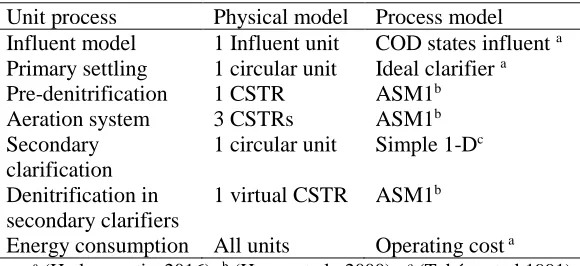
(PPUV) parameter. The sub-models used for each process are summarized in Table 2.

Table 2. Sub-models of the Castiglione Torinese WWTP

Unit process Physical model Process model

Influent model 1 Influent unit COD states influent a

Primary settling 1 circular unit Ideal clarifier a

Pre-denitrification 1 CSTR ASM1b

Aeration system 3 CSTRs ASM1b

Secondary clarification

1 circular unit Simple 1-Dc

Denitrification in secondary clarifiers

1 virtual CSTR ASM1b

13 2.7 Model Calibration

Model calibration is an iterative procedure for adjusting model parameters (physical, operational, kinetic)

to improve the fit to observed set of data. The definition does not include additional measurements and

model structural modification. As a general step-wise calibration procedure in this study, the following

steps were undertaken:

Step 1) The first steady-state simulation of the model was conducted with the reference parameters for a

period equivalent to at least three times the average SRT of the system. and Modelling results were

qualitatively (visual and graphical) compared with available measured data.

Step 2) The most sensitive parameters of each sub-model were detected based on experience and common

sense, engineering judgment, BIOMATH (Vanrolleghem et al., 2003) and STOWA (Hulsbeek et al., 2002)

calibration protocols. In a few cases, full-scale observations and sensitivity analysis using

one-variable-at-a-time approach (Makinia et al., 2005) also contributed in the selection of these parameters.

Step 3) To compensate for the correlational impact of adjusted parameters, first the influent model was

calibrated followed by primary and secondary clarifiers to achieve the solids mass balance in the system.

Further, aeration followed by biokinetic models were calibrated. It should be emphasized that the

calibration of each sub-model is not independent as the modelled processes are coupled together. As a

result, several iterations with loops to the earlier steps were required. Selected parameters in each

sub-model were estimated by a Nelder-Mead simplex (polyhedron) algorithm available in GPS-X. The

methodology is a multi-dimensional method not relying on gradient information for minimization of the

objective function (Press, 2007). The maximum likelihood objective function as well as default values of

reflection, expansion, shrink and contraction constants presented in Hydromantis (2016) were used for

14

literature (e.g. Jeppson, 1996; Henze et al., 2000; Afonso and da Conceição Cunha, 2002) or by

experience. It should be stressed that in case of encountering identifiability problem in which more than

one combination of model parameters could result in a good fit to the observed set of data, the realistic

parameter combinations were identified according to objective of the project and real practical and

theoretical data about the involved process in the plant (Kristensen et al., 1998).

Step 4) The obtained parameters and concentrations from steady state runs in step 3 were used as the initial

conditions for dynamic simulations and the dynamic calibration was performed iterating the procedure in

step 3.

For calibration of the aeration process, initially, α factors (ratio of process water to clean water mass

transfer coefficients) were adjusted to improve the fit to observed set of DO, NH4 and NO3 concentrations

measured in the effluent of each aeration unit. Further, the implemented PI controllers were tuned with

adjustment of the DO setpoint (see section 3.1), proportional gain (Kc) and integral time (Ti) tuning

constants.

The calibration of the EC models was performed considering the specific electricity consumption values

reported in Panepinto et al. (2016) for some of the electro-mechanic devices in the Castiglione Torinese

WWTP. These values were acquired from the tele-control system and some direct measurements to

evaluate overall energy features of the plant. Two calibrating parameters namely pressure drop in piping

and diffuser downstream of blower (PD) and combined blower and motor efficiency (BME) were adjusted,

for calibration of the aeration energy model. The pumping energy models were calibrated by adjustment

of pump efficiency (PE) and pipe friction loss (PFL), assuming constant static system head. Mixing energy

models were calibrated by adjusting power per unit volume (PPUV) parameters. The calibrated parameters

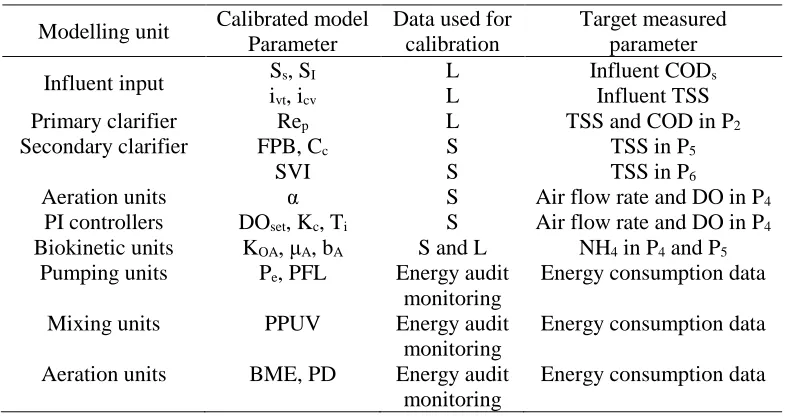
15

Table 3. Calibrated and target parameters

Modelling unit Calibrated model Parameter

Data used for calibration

Target measured parameter

Influent input Ss, SI L Influent CODs

ivt, icv L Influent TSS

Primary clarifier Rep L TSS and COD in P2

Secondary clarifier FPB, Cc S TSS in P5

SVI S TSS in P6

Aeration units α S Air flow rate and DO in P4

PI controllers DOset, Kc, Ti S Air flow rate and DO in P4

Biokinetic units KOA, μA, bA S and L NH4 in P4 and P5

Pumping units Pe, PFL Energy audit

monitoring

Energy consumption data

Mixing units PPUV Energy audit

monitoring

Energy consumption data

Aeration units BME, PD Energy audit

monitoring

Energy consumption data

2.8 Evaluation of the results

The calibrated model was validated to assess the quality of the simulation results by quantifying the

deviations between the model outputs and observations. To this end, the root mean squared error (RMSE)

and the mean absolute percentage error (MAPE) were used as quantitative measures of the model

prediction accuracy with respect to effluent TSS, NH4 and NO3 observations. These statistical criteria

were calculated from Eq. 2 and Eq. 3.

𝑀𝐴𝑃𝐸 =100

𝑛 ∑ |

𝑃𝑡−𝑚𝑡

𝑃𝑡 |

𝑛

𝑡=1 (2)

𝑅𝑀𝑆𝐸 = √∑𝑛𝑡=1(𝑚𝑡−𝑃𝑡)2

𝑛 (3)

where Pt is model predicted output, mt is measured value at the tthtime instance and n is the total number

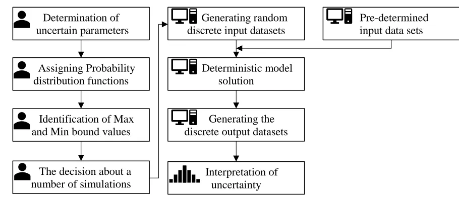
16 2.9 Uncertainty analysis

To assess the input (subjective) uncertainty of the developed model, the Monte Carlo Analysis (MCA)

was performed. MCA provides a probabilistic shell around the deterministic models and quantifies the

uncertainty of the model predictions by expanding the small size sample with the use of probability

distribution functions assigned to input parameters and running several simulations with randomly

selected model inputs (Bixio et al., 2002). Fig. 2 demonstrates the stepwise approach implemented in

MCA.

Fig. 2. Step-wise Monte Carlo analysis

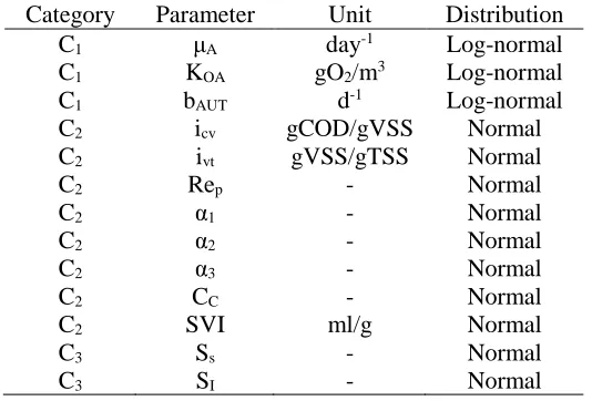
In this study, 13 calibrated parameters (see Table 4) including 7 kinetic and stoichiometric parameters, α

values of aeration basins and 3 operational parameters related to clarifiers were considered as uncertain

input parameters.

Determination of uncertain parameters

Assigning Probability distribution functions

Identification of Max and Min bound values

The decision about a number of simulations

Generating random discrete input datasets

Pre-determined input data sets

Deterministic model solution

Generating the discrete output datasets

17

Table 4. Uncertain parameters and their distribution functions in MCA

These parameters were categorized in 3 uncertainty classes depending on their level of uncertainty and

the extent of available knowledge about them. The first class (C1) corresponded to the numerically

calibrated kinetic parameters. For the parameters in C1 the universal parameter distributions proposed by

Cox (2004) as well as uniform distribution functions were considered. Upper and lower bounds around

their calibrated values were determined according to ranges proposed in the literature (Jeppson, 1996;

Henze et al., 2000; Afonso and da Conceição Cunha, 2002). For the parameters in the second class (C2),

normal distribution functions were assigned with 25% upper and lower bounds around their calibrated

values. The third class (C3) corresponded to 2 influent COD fractions which were obtained by the

calibration process. Parameters in this class were considered as highly uncertain parameters because of

their nature (diurnal, monthly and seasonal variations) and identifiability problems occurred during their

calibration process. For parameters in C3, normal distribution functions were assigned with 50% upper

and lower bounds around their calibrated values. It should be stressed that for the simplicity, parameters

were assumed to be independent and their possible correlations were neglected.

Latin hypercube sampling (LHS) method was implemented for the sampling of the input uncertainty. To

identify the sufficient number of replications in MCA, steady-state simulations were conducted with a

Category Parameter Unit Distribution

C1 μA day-1 Log-normal

C1 KOA gO2/m3 Log-normal

C1 bAUT d-1 Log-normal

C2 icv gCOD/gVSS Normal

C2 ivt gVSS/gTSS Normal

C2 Rep - Normal

C2 α1 - Normal

C2 α2 - Normal

C2 α3 - Normal

C2 CC - Normal

C2 SVI ml/g Normal

C3 Ss - Normal

18

various number of runs (from 100 to 10000) and input probability distribution graphs were developed

accordingly. Graphs were further qualitatively (visual and graphical) analysed and the minimum number

of replications which made the best agreement between assigned distribution function to input variables

and the developed graph, was chosen as the sufficient number of runs. This simplifying method was

chosen considering the available computational power and time of the project. Finally, the results were

represented by mean, 5th _{and 95}th _{percentiles and cumulative distribution functions (CDF).}

3. Results and discussions

3.1 Data collection and practical challenges

Because of the sampling type (daily composite) and location in the plant routine data collection,

the impact of RWS and RWF and wet-weather events could not be captured which makes the historical

data not thoroughly representative of the real condition of the plant. However, modular and temporal

trends of influent flowrate and concentrations in addition to observed ranges for mixed liquor suspended

solids (MLSS) in aeration units and SVI in secondary clarifiers were identified from routinely collected

data which were further elaborated in modelling and calibration (see section 3.3). Since no flow

measurements could be conducted from the effluent of the treatment units, data accuracy evaluation (e.g.

mass balance) could not be scrutinised in both routine data collection and the sampling campaign.

During the additional sampling campaign, mixing deficiency in the anoxic units due to mixer

clogging was frequently observed. Several dead zones and floating sludge areas caused by diffusers

fouling and bulk air emission due to relocated, broken or deformed diffusers bases were noticed in 3

studied aeration tanks.

In the sampling period, managing staff was advised to keep operational conditions of the studied

19

extreme wet-weather events occurred during this period. Since both issues were found very important in

the influent characteristics, recorded results were partitioned into two main categories: the 11-day normal

operational condition in dry weather (NC-D) and the 9-day high load operational condition in wet weather

(HC-W) in which discharge of RWS and heavy rain event occurred. During the 2-day dynamic sampling

campaign the discharge of RWS was recorded in dry weather condition (HC-D). Table 5 shows the

average influent concentrations of the studied module in each operational mode.

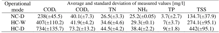
Table 5. Average of the influent concentration in different operational modes observed in sampling campaign period (26.10-21.11.2016)

Operational mode

Average and standard deviation of measured values [mg/l]

CODt CODs TN NH4 TP TSS

NC-D 238(±45.5) 40.1(±7.3) 26.5(±3.3) 25.2(±0.05) 3.7(±2.7) 134.7(±37.9)

HC-W 407(±110.2) 41.9(±4.2) 34.6(±4.6) 29.3(±0.1) 7(±3.7) 274.1(±95.1)

HC-D 734(±135.7) 73.2(±13.2) 44.5(±4.2) 38.4(±2.2) 9(±1.8) 442(±95.1)

Partitioned results highlight the impact of RWS on influent characteristics since concentrations

recorded in NC-D were found almost doubled or tripled in HC-D operational mode. Moreover, the dilution

effect of a wet weather event on influent concentrations can be clearly detected, comparing the results

recorded in HC-D and HC-W modes. Considering the high deviation of influent concentrations in various

operational modes, it was decided to use collected data in NC-D mode for model calibration. The data

collected in HC-D and HC-W modes were further elaborated in model-based optimization and scenario

planning in an accompanying study (Borzooei et al., in preparation) to keep this study focused on the

framing of the model development and calibration.

The collected data was further analysed to investigate the performance of treatment units.

Comparing the CODs, NH4 concentrations recorded in P2 and P3 (see Fig. 1), the reactive nature of the

primary clarifier was revealed with 270 and 110 kg/d increasing of the NH4 and CODs loads respectively.

Comprehensive investigation of the reactive primary clarifier was performed in Borzooei et al. (2017).

20

average, the occurrence of denitrification during the studied period was confirmed. A tentative study based

on decision tree proposed in Comas et al. (2008) was performed to evaluate the risk of rising sludge. The

results confirmed the high risk of sludge rising in denitrifying clarifiers as a result of their high residence

time and the influent nitrate level above the critical value (Henze et al., 1993). However, to certainly link

the sludge rising phenomena, which were frequently observed in the plant, to the denitrification process,

further investigation was proposed.

A high discrepancy was observed between online measurements of NH4 and lab analyses of grab

samples collected from the effluent of aeration units (P4). These discrepancies resulted from the

occurrence of several types of sensors failure including a long period with sensor fault (constant value) as

well as periodic faults (incorrect scaling and/or out of normal range values) during the campaign (see Fig

A. 2). Therefore, lab resultswere used for calibration process. Considering the performance of NH4 sensor

and investigating the DO concentrations and airflow rate recorded in the sampling period, it was induced

that ammonium-based supervisory control system was not really implemented in controlling of the

aeration systems, rather they were controlled manually.

3.2 Wastewater and biomass characterization

The initial fractionation of organic matter in influent wastewater was carried out according to methods

proposed by standard Dutch guidelines (Roeleveld and Van Loosdrecht, 2002). Obtained results are

presented in Table 1. The average contribution of individual ASM1 components to total COD was found

as follows: SI = 1.1%, Ss = 9.1%, Xs = 44 %, XI = 45.8 %. The estimated Ss fraction corresponds to a low

value but still within the reported range in several studies (e.g. Henze, 1992; Chachuat et al., 2005;

Marquot et al., 2006; Pasztor et al., 2009) in which Ss constituted 3-35% and 14-57% of total COD in raw

municipal and settled wastewater respectively. However, the estimated SI fraction was found to be out of

21

2009). To solve the identifiability problem in the calibration of the influent model (see Table 3), SI value

was numerically calibrated while Ss was kept unchanged. The adjusted SI value remained in the suggested

range. The estimated XI/total COD ratio (45.8%) was higher than the reported range (8-39%) (Henze,

1992; Roeleveld and Van Loosdrecht, 2002). The high XI value can be linked to two factors: long

hydraulic residence time in sewage pipelines and share of industrial wastewater in the. As proposed in

several studies (e.g. Szaja et al., 2015; Pasztor et al., 2009; Quevauviller et al., 2007), for the large WWTPs

like Castiglione Torinese which have more complex sewer collection system with a longer retention time

of wastewater, the biological degradation of substrate fraction occur at bigger scale in sewer system which

results the increase of inert particulate components. The higher inert COD fraction can be also linked with

a presence of industrial wastewater (Mhlanga and Brouckaert, 2013). In the case of this study, Castiglione

Torinese is the municipal WWTPs with a dominant contribution of non-industrial discharges in the

wastewater influent.

The first estimated Xs/XI ratio was revised based on calibration of the influent model. The Xs fraction was

reduced from 44% to 37%. After this adjustment, Xs fraction remained within the typical range of 28-68%

(Kappeler and Gujer, 1992; Roeleveld and Van Loosdrecht, 2002). Although the Ss/(Ss+Xs) ratio was

improved with the adjustment but it is still out of the typical range of 0.3-0.5 reported in Makinia et al.

(2006). It should be emphasized that autotrophic (XBA) and heterotrophic (XBH) biomass concentrations

were assumed equal to 0.1-1 and 0 mg/l respectively because these two fractions are included in particulate

22 3.3 Model calibration

The model was calibrated under a dynamic condition with the data originating from both laboratory and

sensor readings on NC-D operational mode in the sampling period (26.10-21.11.2016) following the

approach presented before. The final set of adjusted parameters and their original values are tabulated in

Table 6. After the adjustment of two COD fractions (SI and SS) according to CODs measurements, the

influent model was calibrated by increasing icv to 1.85gCOD. (gVSS)-1 which was assumed based on the

measurement of the CODt and MLVSS in the aeration tanks while keeping ivt constant.

In the calibration of the secondary clarifier model, clarification coefficient (Cc) was decreased to 0.42 to

improve the final effluent TSS model prediction. The SVI was decreased from 150 to 130 ml/ to calibrate

the sludge thickening process in the secondary clarifier and improve the fit to observed TSS values in

RAS. The adjusted SVI value remained in obtained range (85-148 ml/g) from routine data collection (see

section 2.2).

The calibrated α values for 3 aeration basins indicated higher aeration efficiency of one of the tanks in

comparison to others. Since fouling factor (Ff) equal to 1 was assumed for all three tanks, the differences

23

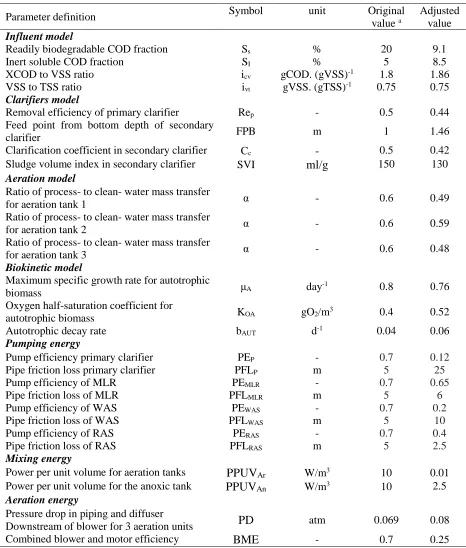
Table 6. Original and adjusted parameters in the calibration process

Parameter definition Symbol unit Original

value a

Adjusted value

Influent model

Readily biodegradable COD fraction Ss % 20 9.1

Inert soluble COD fraction SI % 5 8.5

XCOD to VSS ratio icv gCOD. (gVSS)-1 1.8 1.86

VSS to TSS ratio ivt gVSS. (gTSS)-1 0.75 0.75

Clarifiers model

Removal efficiency of primary clarifier Rep - 0.5 0.44

Feed point from bottom depth of secondary

clarifier FPB m 1 1.46

Clarification coefficient in secondary clarifier Cc - 0.5 0.42

Sludge volume index in secondary clarifier SVI ml/g 150 130

Aeration model

Ratio of process- to clean- water mass transfer

for aeration tank 1 α - 0.6 0.49

Ratio of process- to clean- water mass transfer

for aeration tank 2 α - 0.6 0.59

Ratio of process- to clean- water mass transfer

for aeration tank 3 α - 0.6 0.48

Biokinetic model

Maximum specific growth rate for autotrophic

biomass μA day

-1 _{0.8 0.76}

Oxygen half-saturation coefficient for

autotrophic biomass KOA gO2/m

3 _{0.4 0.52}

Autotrophic decay rate bAUT d-1 0.04 0.06

Pumping energy

Pump efficiency primary clarifier PEP - 0.7 0.12

Pipe friction loss primary clarifier PFLP m 5 25

Pump efficiency of MLR PEMLR - 0.7 0.65

Pipe friction loss of MLR PFLMLR m 5 6

Pump efficiency of WAS PEWAS - 0.7 0.2

Pipe friction loss of WAS PFLWAS m 5 10

Pump efficiency of RAS PERAS - 0.7 0.4

Pipe friction loss of RAS PFLRAS m 5 2.5

Mixing energy

Power per unit volume for aeration tanks PPUVAr W/m3 10 0.01

Power per unit volume for the anoxic tank PPUVAn W/m3 10 2.5

Aeration energy

Pressure drop in piping and diffuser

Downstream of blower for 3 aeration units PD atm 0.069 0.08

Combined blower and motor efficiency BME - 0.7 0.25

24

The nitrification process was initially calibrated by decreasing the maximum specific growth rate for

autotrophic biomass (μA) from 0.8 to 0.76 (d-1) to improve the modelling results fit to the observed set of

the ammonia level at the effluent of aeration tanks. It should be also mentioned that the nitrate

concentration in aeration tanks was slightly decreased by adjusting the μA. This value corresponds to the

reported range (0.2-1.2 d-1) (Henze et al., 2000; Afonso and da Conceição Cunha, 2002). The ammonia and nitrate fits were further improved by increasing the autotrophic decay rate (bA) from 0.04 to 0.06 (d -1_{) and oxygen half-saturation index for autotrophic biomass (K}

OA) from 0.4 to 0.52 gO2/m3. A higher

estimated bA value can be the result of the long oxic-SRT of the system (average 30 days)

(Liwarska-Bizukojc et al., 2011). As stated in Arnaldos et al. (2015), several factors influence half saturation index

including factors involved in transport in the bulk medium, into the floc, through the cell membrane, in

the periplasm and enzymatic binding/release of a substrate. However, among all the influencing factors,

the bulk mixing condition is logically the first factor to be investigated since its impact may overwhelm

the contributions of other factors especially in case of non-uniform mixing condition. Since actual dead

zones were observed in aeration tanks in the Castiglione Torinese plant during the sampling campaign;

the advection limitation can be the explanation for the need to increase the KOA. Both adjusted parameters

(bA and KOA) corresponded well within the reported ranges (Henze et al., 2000; Jeppson, 1996). In the

calibration of the pumping EC models, since no practical information was available about real PE and

PFL values, one of their obtained combinations in the parameter estimation process was used. However,

for calibration of the aeration EC model, based on the sensitivity analysis results, initially, the PD

parameter was adjusted followed by BME.

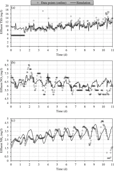
3.3 Evaluation of modelling results

The results of the dynamic simulations for 3 effluent concentrations (TSS, NH4 and NO3) are presented in

25

(Fig. 3a) and expressed by the low values of the MAPE = 19 % and RMSE = 0.33 mg/l. It should be noted

that a short period of sensor failure (constant value) in the first two days of the sampling affected the

model evaluation results.

For both the description of the effluent NO3 and NH4, even though the differences between online data

and model prediction were relatively higher (MAPE = 11-34 % and RMSE= 0.14-1.5 mg/l respectively),

the model predictions reasonably follow the trend of the actual data (Fig. 3 b and c). However, the model

frequently overpredicted the NO3 level in the afternoon (from 14:00 pm) on each simulating day where

real data showed drops and lower values. A possible reason could be the increased residence time (lower

flow rate in afternoons) in the aeration tanks through which simultaneous denitrification can take place,

especially in the dead zones in presence of enough readily biodegradable COD which is not captured by

the way the mixing is currently modelled. Besides, in the ASM1 the same oxygen half saturation

coefficient for heterotrophs (KOH) is considered for modelling both the aerobic and anoxic growth of

heterotrophic biomass. Hence, in the modelling approach, if aerobic growth of heterotrophs decreases, the

capacity for anoxic growth will increase. This emphasizes the importance of KOH in calibration process

which was kept constant in this study due to data scarcity. Moreover, considering the occurrence of the

denitrification in secondary clarifiers during the sampling campaign, a lower flow rate can result in the

higher sludge residence time in the clarifier and consequently intensify the denitrification.

Since the calibration process was conducted based on the results of composite samples, logically the

events with fast dynamics could not be well-captured by the developed model; however, the data with

abrupt changes, disturbance and fluctuations in plant record data brought additional difficulties in the

calibration process and parameter estimation. The removal efficiencies for effluent parameters were

calculated based on actual measurement and dynamically simulated average values. The results proved

26

Fig. 3. Measurements vs. model predictions of effluent TSS (a), N-NO3 (b), N-NH4 (c) within the sampling campaign period (26.10-21.11.2016)

0 2 4 6 8 10 12 14 16 18 20

0 1 2 3 4 5 6 7 8 9 10 11

Eff

luent

TS

S

(m

g/

l)

Time (d)

Data points (online) Simulation

(a)

4 4.5 5 5.5 6 6.5 7 7.5 8 8.5 9

0 1 2 3 4 5 6 7 8 9 10 11

Eff

luent

NO

3

(m

g/

l)

Time (d)

(b)

0 0.5 1 1.5 2 2.5 3 3.5 4 4.5 5

0 1 2 3 4 5 6 7 8 9 10 11

Eff

luent

NH

4

(m

g/

l)

Time (d)

27

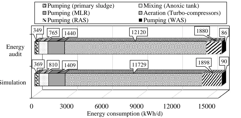
EC modelling results confirmed that aeration and pumping systems are the biggest energy consumers with

70-78% and 20-26 % of the total energy consumption of the studied module respectively. Measured and

simulated daily averaged EC of treatment units were calculated (Fig. 4). The results presented in Fig. 4

proved that the model predictions are in relatively good agreement with energy audit data.

Fig. 4. Comparison of the measured and simulated daily averaged energy consumption of the studied module

3.4 Uncertainty assessment and improving proposals

To evaluate the uncertainty analysis results, CDFs of aggregated measure of averaged effluent TSS, CODt,

NO3 and NH4 concentrations were developed (Fig. 5). Comparing the results of the base-case simulation

(Fig. 4) and the results presented in Fig. 5, one observes that there is considerable uncertainty concerning

all effluent parameters. These results proved that uncertainty of the kinetic, stoichiometric, influent

fractions and operational parameters cause significant variance in the predicted effluent concentrations.

As regards the CDF of the effluent TSS (Fig. 5a) it can be noted that the spread of uncertainty is very

broad. This can be due to two main reasons: (i) No MLSS controller was implemented in the model to

counteract the uncertainty in the input parameters and as a result maintaining relatively stable MLSS level

(ii) uncertainty of the operational input parameters regarding secondary and primary clarifiers.

0 3000 6000 9000 12000 15000

Simulation Energy

audit

369 349

810 765

1409 1440

11729 12120

1898 1880

90 86

Energy consumption (kWh/d)

Pumping (primary sludge) Mixing (Anoxic tank)

Pumping (MLR) Aeration (Turbo-compressors)

28

Fig. 5. Representations of uncertainty in four effluent parameters by the cumulative distribution function (CDF)

Conducting settling tests as well as representative COD fractionation and measuring campaigns

associated with each operational mode and the tracer test to set-up an accurate hydraulic model for

clarifiers were proposed to reduce the uncertainty the modelling results. Likewise, a wide range of

uncertainty was observed in predicted effluent COD and nitrogen concentrations which can be linked to

all sources of the uncertainty although the impact of operational parameters of clarifiers and mass transfer

related parameters may be overwhelmed (Sin et al., 2009). Beside above-mentioned additional tests,

application of the DO, NO3, NH4, TSS in-situ probes and actual implemented airflow controlling system

0.0 0.2 0.4 0.6 0.8 1.0

5 35 65 95 125 155 185

C um ul at iv e pr obabi li ty

Effluent TSS (mg/l)

(a) 0.0 0.2 0.4 0.6 0.8 1.0

10 40 70 100 130 160 190 220

Cum ul at iv e p rob ab il it y

Effluent total COD (mg/l)

(b) 0.0 0.2 0.4 0.6 0.8 1.0

0 2 4 6 8 10 12 14 16

C um ul at iv e pr obabi li ty

Effluent Nitrate (mgN/l)

(c) 0.0 0.2 0.4 0.6 0.8 1.0

0 5 10 15 20 25 30

C um ul at iv e pr obabi li ty

Effluent Ammonium (mgN/l)

29

in aeration units and conducting series of experimental batch tests to measure the kinetics parameters were

proposed to improve the certainty of the modelling results.

5. Conclusions

This study proposes a novel methodology to address the impact of data quality and quantity

problems on modelling and calibration of WWTPs. Historical data of the large-scale Castiglione Torinese

WWTP, from January 2009 to December 2016, in addition to data collected in a few sampling and

measurement campaigns, were utilized for model development and calibration. Unprecedented changes

in weather condition, sensor performance and discharge of reject water from sludge treatment units during

the sampling campaign were found intensifying sources of data scarcity in this project. The practical

information presented in this study, stresses the role of a well-designed data collection process for both

performance investigation and troubleshooting of treatment units which is usually overlooked, or its

importance underestimated. The reactive nature of the primary clarifier and denitrification in the

secondary clarifier were identified based on sampling campaign results. The developed model comprises

biokinetic, aeration, hydraulic and transport, clarifier, input, output and energy consumption sub-models,

and was calibrated by use of an extensive step-wise calibration process. Short-term predictability of the

calibrated model was confirmed by comparing the dynamics of simulated and measured TSS, N-NH4 and

N-NO3 effluent concentrations as well as their removal efficiencies. The uncertainty of the model was

investigated by Monte Carlo Analysis (MCA). The results of the MCA emphasized the impact of data

quality and quantity problem on uncertainty of developed model by showing high variances of effluent

concentrations in MCA results. Considering the MCA results, additional tests, sampling and

30 6. Acknowledgments

This research was financially supported by Società Metropolitana Acque Torino (SMAT). The authors

wish to thank all the SMAT laboratory, maintenance and operations personnel for their engagement and

31 References:

Arnaldos, M., Amerlinck, Y., Rehman, U., Maere, T., Van Hoey, S., Naessens, W., and Nopens, I. (2015). From the affinity constant to the half-saturation index: Understanding conventional modeling concepts in novel wastewater treatment processes. Water Res. 70, 458–470.

Balku S, Berber R (2006). Dynamics of an activated sludge process with nitrification and denitrification: Start-up simulation and optimization using evolutionary algorithm. Computer and Chemical Engineering, 30(3), pp. 490-499.

Beraud, B. (2009). Methodology for the optimization of wastewater treatment plant control laws based on modeling and multi-objective genetic algorithms. Université Montpellier II-Sciences et Techniques du Languedoc.

Bixio, D., Parmentier, G., Rousseau, D., Verdonck, F., Meirlaen, J., Vanrolleghem, P.A., and Thoeye, C. (2002). A quantitative risk analysis tool for design/simulation of wastewater treatment plants. Water Sci. Technol. 46, 301–307.

Blundo, C.M., Campanella, L., Capri, S., La Noce, T., Liberatori, A., Pagnotta, R., and Pettine, M. (1994). Metodi analitici per Acque. Man. IRSA–CNR Ist. Poligr. E Zecca Dello Stato Roma.

Borzooei, S., Zanetti, M.C., Genon, G., Ruffino, B., Godio, A., Campo, G., Panepinto, D., Lorenzi, E., De Ceglia, M., and Binetti, R. (2016), Modelling and calibration of the full-scale WWTP with data scarcity. Proceedings of International Symposium on sanitary and environmental engineering, Rome.

Borzooei, S., Zanetti, M.C., Lorenzi, E., and Scibilia, G. (2017). Performance Investigation of the Primary Clarifier-Case Study of Castiglione Torinese. In Frontiers International Conference on Wastewater Treatment and Modelling, (Springer), pp. 138–145.

Bott, C.B., and Parker, D.S. (2011). WEF/WERF study quantifying nutrient removal technology performance (Water Environment Research Foundation Alexandria, VA).

Chachuat, B., Roche, N., and Latifi, M.A. (2005). Long-term optimal aeration strategies for small-size alternating activated sludge treatment plants. Chem. Eng. Process. Process Intensif. 44, 591–604.

Comas, J., Rodríguez-Roda, I., Gernaey, K.V., Rosen, C., Jeppsson, U., and Poch, M. (2008). Risk assessment modelling of microbiology-related solids separation problems in activated sludge systems. Environ. Model. Softw. 23, 1250–1261.

Cox, C.D. (2004). Statistical distributions of uncertainty and variability in activated sludge model parameters. Water Environ. Res. 76, 2672–2685.

32

Ferrer, J., Morenilla, J.J., Bouzas, A., and Garcia-Usach, F. (2004). Calibration and simulation of two large wastewater treatment plants operated for nutrient removal. Water Sci. Technol. 50, 87–94.

Gernaey, K.V., van Loosdrecht, M.C., Henze, M., Lind, M., and Jørgensen, S.B. (2004). Activated sludge wastewater treatment plant modelling and simulation: state of the art. Environ. Model. Softw. 19, 763– 783.

Henze, M. (1992). Characterization of wastewater for modelling of activated sludge processes. Water Sci. Technol. 25, 1–15.

Henze, M., Dupont, R., Grau, P., and De La Sota, A. (1993). Rising sludge in secondary settlers due to denitrification. Water Res. 27, 231–236.

Henze, M., Gujer, W., Mino, T., and Van Loosdrecht, M.C.M. (2000). Activated sludge models ASM1, ASM2, ASM2d and ASM3 (IWA publishing).

Hulsbeek, J.J.W., Kruit, J., Roeleveld, P.J., and Van Loosdrecht, M.C.M. (2002). A practical protocol for dynamic modelling of activated sludge systems. Water Sci. Technol. 45, 127–136.

Hydromantis Environmental Software Solutions, Inc. (2016). GPS-X Version 6.5: GPS-X Technical Reference. Ontario, Canada.

Jeppson, U. (1996). Modeling aspects of wastewater treatement plants. PhD thesis, IAE, Lund, Sweden.

Kappeler, J., and Gujer, W. (1992). Estimation of kinetic parameters of heterotrophic biomass under aerobic conditions and characterization of wastewater for activated sludge modelling. Water Sci. Technol.

25, 125–139.

Kristensen, G.H., la Cour Jansen, J., and Jørgensen, P.E. (1998). Batch test procedures as tools for calibration of the activated sludge model-A pilot scale demonstration. Water Sci. Technol. 37, 235–242.

Langergraber, G., Rieger, L., Winkler, S., Alex, J., Wiese, J., Owerdieck, C., Ahnert, M., Simon, J., and Maurer, M. (2004). A guideline for simulation studies of wastewater treatment plants. Water Sci. Technol.

50, 131–138.

Liu, C., Li, S., and Zhang, F. (2011). The oxygen transfer efficiency and economic cost analysis of aeration system in municipal wastewater treatment plant. Energy Procedia 5, 2437–2443.

Liwarska-Bizukojc, E., Olejnik, D., Biernacki, R., and Ledakowicz, S. (2011). Calibration of a complex activated sludge model for the full-scale wastewater treatment plant. Bioprocess Biosyst. Eng. 34, 659– 670.

Makinia, J., Rosenwinkel, K.-H., and Spering, V. (2005). Long-term simulation of the activated sludge process at the Hanover-Gümmerwald pilot WWTP. Water Res. 39, 1489–1502.

33

Marquot, A., Stricker, A.-E., and Racault, Y. (2006). ASM1 dynamic calibration and long-term validation for an intermittently aerated WWTP. Water Sci. Technol. 53, 247–256.

Martin, C., and Vanrolleghem, P.A. (2014). Analysing, completing, and generating influent data for WWTP modelling: a critical review. Environ. Model. Softw. 60, 188–201.

Melcer, H. (2004). Methods for wastewater characterization in activated sludge modelling (IWA publishing).

Mhlanga, F.T., Brouckaert, C.J., 2013. Characterisation of wastewater for modelling of wastewater treatment plants receiving industrial effluent. Water SA 39, 403–408.

Mueller, J., Boyle, W.C., and Popel, H.J. (2002). Aeration: Principles and practice (CRC press).

Murphy, K.L., and Boyko, B.I. (1970). Longitudinal mixing in spiral flow aeration tanks. J. Sanit. Eng. Div. 96, 211–221.

Panepinto, D., Fiore, S., Zappone, M., Genon, G., and Meucci, L. (2016). Evaluation of the energy efficiency of a large wastewater treatment plant in Italy. Appl. Energy 161, 404–411.

Pasztor, I., Thury, P., and Pulai, J. (2009). Chemical oxygen demand fractions of municipal wastewater for modeling of wastewater treatment. Int. J. Environ. Sci. Technol. 6, 51–56.

Press, W.H. (2007). Numerical recipes 3rd edition: The art of scientific computing (Cambridge university press).

Quevauviller, P., Thomas, O., Van Der Beken, A., 2007. Wastewater quality monitoring and treatment. John Wiley & Sons.

Rieger, L., Takacs, I., Shaw, A., Winkler, S., Ohtsuki, T., Langergraber, G., Gillot, S., and Models, I.T.G. on G.M.P.G. for U. of A.S. (2010a). Status and future of wastewater treatment modelling (IWA Publishing).

Rieger, L., Takács, I., Villez, K., Siegrist, H., Lessard, P., Vanrolleghem, P.A., and Comeau, Y. (2010b). Data reconciliation for wastewater treatment plant simulation studies-planning for high-quality data and typical sources of errors. Water Environ. Res. 82, 426–433.

Roeleveld, P.J., and Van Loosdrecht, M.C.M. (2002). Experience with guidelines for wastewater characterisation in The Netherlands. Water Sci. Technol. 45, 77–87.

Schilperoort, R.P.S. (2011). Monitoring as a tool for the assessment of wastewater quality dynamics. PhD thesis, Water Management Academic Press - Delft, the Netherlands.

Sin, G., Gernaey, K.V., Neumann, M.B., van Loosdrecht, M.C., and Gujer, W. (2009). Uncertainty analysis in WWTP model applications: a critical discussion using an example from design. Water Res.

34

Sochacki, A., Knodel, J., Gei\s sen, S.U., Zambarda, V., Miksch, K., and Bertanza, G. (2009). Modelling and simulation of a municipal WWTP with limited operational data. In Proceedings of a Polish-Swedish-Ukrainian Seminar, pp. 23–25.

Szaja, A., Aguilar, J.A., Lagód, G., 2015. Estimation of Chemical Oxygen Demand Fractions of Municipal Wastewater by Respirometric Method–Case Study. Rocz. Ochr. Śr. 17, 289–299.

Takács, I., Patry, G.G., and Nolasco, D. (1991). A dynamic model of the clarification-thickening process. Water Res. 25, 1263–1271.

Vanrolleghem, P.A., Insel, G., Petersen, B., Sin, G., De Pauw, D., Nopens, I., Dovermann, H., Weijers, S., and Gernaey, K. (2003). A comprehensive model calibration procedure for activated sludge models. Proc. Water Environ. Fed. 2003, 210–237.

Zawilski, M., Brzezińska, A., 2009. Variability of COD and TKN Fractions of Combined Wastewater. Pol. J. Environ. Stud. 18.

Zima, P., Makinia, J., Swinarski, M., and Czerwionka, K. (2008). Effects of different hydraulic models on predicting longitudinal profiles of reactive pollutants in activated sludge reactors. Water Sci. Technol.

35

Appendix:

Fig. A.1. Comparison of sensor and sampling results for effluent NH4 at 3 aeration tanks within the sampling campaign period (26.10-21.11.2016)

0 5 10 15 20 25 30 35

0.0 2.0 4.0 6.0 8.0 10.0

NH

4

C

once

nt

rat

ion

(m

g

/l

)

Time (d)

Aeration tank 1 (sensor) Aeration tank 2 (sensor)

Aeration tank 3 (sensor) Aeration tank 1 (sampling)