Numerical Simulation of Wave-Plasma
Interactions in the Ionosphere
by
Patrick David Cannon
A thesis submitted in partial fulfillment for the degree of Doctor of Philosophy
in the
Faculty of Science and Technology Department of Physics
I, Patrick David Cannon, declare that this thesis titled,‘Numerical Simulation of Wave-Plasma Interactions in the Ionosphere’ and the work presented in it are my own. I confirm that:
This work was done wholly or mainly while in candidature for a research degree at this University.
Where any part of this thesis has previously been submitted for a degree or any other qualification at this University or any other institution, this has been clearly stated.
Where I have consulted the published work of others, this is always clearly at-tributed.
Where I have quoted from the work of others, the source is always given. With the exception of such quotations, this thesis is entirely my own work.
I have acknowledged all main sources of help.
Where the thesis is based on work done by myself jointly with others, I have made clear exactly what was done by others and what I have contributed myself.
Signed:
Date:
‘but it doesn’t alter facts.’”
Queen’s Play
Ionospheric modification by means of high-power electromagnetic (EM) waves can result in the excitation of a diverse range of plasma waves and instabilities. This thesis presents the development and application of a GPU-accelerated finite-difference time-domain (FDTD) code designed to simulate the time-explicit response of an ionospheric plasma to incident EM waves. Validation tests are presented in which the code achieved good agreement with the predictions of plasma theory and the computations of benchmark software.
The code was used to investigate the mechanisms behind several recent experimental observations which have not been fully understood, including the effect of 2D density inhomogeneity on the O-mode to Z-mode conversion process and thus the shape of the conversion window, and the influence of EM wave polarisation and frequency on the growth of density irregularities.
The O-to-Z-mode conversion process was shown to be responsible for a strong depen-dence of artificially-induced plasma perturbation on both the EM wave inclination angle and the 2D characteristics of the background plasma. Allowing excited Z-mode waves to reflect back towards the interaction region was found to cause enhancement of the electric field and a substantial increase in electron temperature.
Simulations of O-mode and X-mode polarised waves demonstrated that both are capa-ble of exciting geomagnetic field-aligned density irregularities, particularly at altitudes where the background plasma frequency corresponds to an electron gyroharmonic. In-clusion of estimated electrostatic fields associated with irregularities in the simulation algorithm resulted in an enhanced electron temperature. Excitation of these density features could address an observed asymmetry in anomalous absorption and recent un-explained X-mode heating results reported at EISCAT.
The PhD process is a journey that cannot be made alone; I am indebted to many heroic individuals who have helped me immeasurably along the way:
Firstly I would like to thank my supervisor, Prof. Farideh Honary, for giving me an opportunity to study at Lancaster University and for being a constant source of support, guidance and good advice throughout my PhD.
I am grateful to those with whom I have collaborated during my PhD research, par-ticularly to Prof. Nikolay Borisov for taking the time to read and contribute to my article manuscript, and to the staff at the Lancaster University High-End Cluster for their patience and technical assistance. I would also like to thank all members, past and present, of the research group formerly known as SPEARS, who have helped make working at Lancaster a thoroughly enjoyable experience.
That my sanity has been maintained during the past few years is in part thanks to Rowan, Richy and Tom (and around 30,726 unfortunate zombies).
Special thanks are due to those back in the Shire, family and faithful hounds all: it has been a great comfort to know that there is always an unlocked door, a warm fire and a healthy dram waiting just up the road.
Finally, especially, I would like to thank Janette Mill, who would have carried me all the way to Mordor on her own if necessary; without her encouragement and companionship this thesis could have never have been written.
Declaration of Authorship i
Abstract iii
Acknowledgements iv
List of Figures viii
List of Tables xix
Abbreviations xx
1 Introduction: Plasma Physics and the Ionosphere 1
1.1 Plasma Fundamentals . . . 2
1.1.1 Quasi-neutrality and the Debye Length . . . 2
1.1.2 Plasma Parameter . . . 5
1.1.3 Cold Plasma Oscillation . . . 6
1.2 Single-Particle Motion . . . 9
1.2.1 Lorentz Motion and Gyration . . . 9
1.2.2 Guiding Centre Drift . . . 11
1.3 Plasma Dynamics . . . 16
1.3.1 Kinetic Formulation . . . 16
1.3.2 Fluid Formulation . . . 18
1.4 Waves in Plasma . . . 19
1.4.1 Electromagnetic Waves . . . 21
1.4.1.1 Unmagnetised Plasma . . . 21
1.4.1.2 Magnetised Plasma . . . 23
1.4.1.3 EM Waves in a Vertically-Stratified Magnetised Plasma . 29 1.4.2 Electrostatic Electron Waves . . . 32
1.4.3 Ion Waves . . . 36
1.4.4 Kinetic Waves . . . 40
1.4.4.1 Landau Damping . . . 41
1.4.4.2 Cyclotron Damping . . . 43
1.4.4.3 Bernstein Waves . . . 44
1.5 Earth’s Ionosphere and Near-Space Environment . . . 47
1.5.2 The Ionosphere . . . 50
1.6 Ionospheric Modification Experiments . . . 53
1.6.1 E-Field Amplitude Swelling . . . 54
1.6.2 Linear Mode Conversion . . . 56
1.6.3 Plasma Modification . . . 57
1.6.4 Parametric Instabilities . . . 60
1.6.5 Thermal Resonance Instabilities . . . 63
1.6.6 Self-Focusing Instabilities . . . 64
2 Introduction: Numerical Simulation 65 2.1 The Finite-Difference Time-Domain Method . . . 66
2.1.1 Discretisation and the Yee Cell . . . 67
2.1.2 Finite-Difference Approximation . . . 69
2.1.3 Update Equations for Electromagnetic Waves . . . 71
2.2 Dispersion and Stability . . . 75
2.2.1 Dispersion in the FDTD Domain . . . 75
2.2.2 Stability Criteria and the Courant-Friedrichs-Lewy Condition . . . 82
2.2.3 Choosing Simulation Parameters . . . 84
2.3 Boundary Conditions . . . 85
2.3.1 Mur Absorbing Boundary Conditions . . . 86
2.3.2 Perfectly-Matched Layer . . . 89
2.4 FDTD Advantages and Limitations . . . 94
3 Development of a GPU-Accelerated FDTD Scheme for Electromag-netic Wave Interaction with Plasma 98 3.1 Introduction . . . 98
3.2 Methodology . . . 101
3.2.1 Governing Equations . . . 101
3.2.2 Discretisation Scheme . . . 102
3.2.2.1 Update Equation for Magnetic Field . . . 103
3.2.2.2 Update Equation for Electric Field . . . 103
3.2.2.3 Update Equation for Fluid Velocity . . . 103
3.2.2.4 Update Equation for Plasma Density and Temperature . 107 3.2.2.5 Full Update Algorithm . . . 109
3.2.3 Stability and Accuracy . . . 109
3.3 Computational Performance . . . 116
3.4 Validation . . . 121
3.4.1 Wave Propagation Through Homogeneous Plasma . . . 121
3.4.2 Wave Propagation Through Inhomogeneous Plasma . . . 129
3.5 Summary and Conclusions . . . 133
4 Simulation of the Radio Window and Magnetic Zenith Effect 135 4.1 Introduction . . . 135
4.2 Methodology . . . 139
4.3 Numerical Simulation of Radio Window . . . 142
4.4 Impact of Z-mode on Heating Effects . . . 155
4.6 Summary and Conclusions . . . 176
5 Simulation of Density Irregularity Growth During O-Mode and X-Mode Heating 182 5.1 Introduction . . . 182
5.2 Methodology . . . 188
5.3 Excitiation of Density Irregularities . . . 190
5.4 Contribution of Electrostatic Fields to Temperature . . . 212
5.5 Summary and Conclusions . . . 217
6 Comparison of Simulated X-mode Wave Fields with Theoretical Para-metric Instability Thresholds 221 6.1 Introduction . . . 222
6.2 Threshold Calculation and Comparison to Experiment and Observation . 223 6.3 Numerical Simulation Results . . . 228
6.4 Summary and Conclusions . . . 232
7 Summary and Conclusions 234 7.1 Development of a GPU-Accelerated FDTD Scheme . . . 235
7.2 Simulation of the Radio Window and Magnetic Zenith Effect . . . 236
7.3 Simulation of Density Irregularity Growth During O-Mode and X-Mode Heating . . . 239
7.4 Comparison of Simulated X-mode Wave Fields with Theoretical Paramet-ric Instability Thresholds . . . 240
7.5 Further Investigation . . . 242
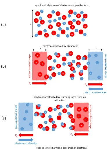
1.1 Schematic diagram of the fundamental cold plasma oscillation in response to the displacement of electrons by an external field. . . 7 1.2 Schematic diagram of an electron moving in a uniform, time-invariant
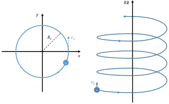
B-field, B = Bˆz. Presence of a magnetic field causes the electron to rotate in a plane perpendicular to the field direction. Motion parallel to the magnetic field combined with simultaneous gyrorotation in the perpendicular plane leads to helical motion of the particle following the field direction. A positive ion would rotate in the opposite sense to the electron due to their opposing polarities. . . 11 1.3 Schematic diagram of electron and ion drift motion for the cases of no
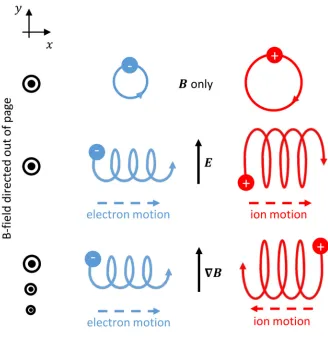
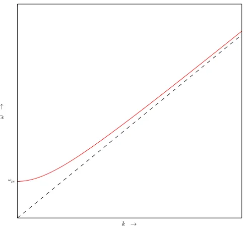
perpendicular field, a perpendicular E-field and a perpendicular B-field gradient. (note that this is a cartoon only: the gyroradii are not to scale) 13 1.4 Dispersion relation for electromagnetic waves in a cold, collisionless,
un-magnetised plasma (red). There is a frequency cut-off at ω=ωpe, below which there is no wave propagation. The relationship asymptotically ap-proaches the ω =ck vacuum expression as frequency is increased (indi-cated by dashed-black line). . . 23 1.5 Dispersion relation for electromagnetic waves in a cold, collisionless,
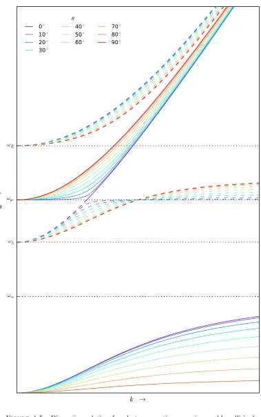
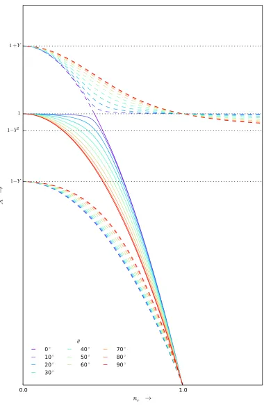
mag-netised plasma for a range of propagation angles between θ= 0 (parallel) and θ = π/2 (perpendicular). The effect of the anisotropy introduced by the static background magnetic field is to split EM wave propagation into several distinct modes determined by polarisation and direction. The solid lines show the “+” solutions from the Appleton-Hartree equation (1.73) (referred to in this thesis as O-modes), while the dashed lines show the“-” solutions (referred to in this thesis as X-modes). . . 27 1.6 Real part of the refractive indexn=nr+ini =c2k2/ω2 for EM waves in a
cold, collisionless, magnetised plasma where the electron density gradient increases linearly along the magnetic field direction, plotted for a range of propagation angles. The O-mode branch is indicated by the solid lines, and shows a clear cut-off at X = 1. The X-mode branches are indicated by dashed lines and show cut-offs at X = 1±Y, and a resonance at X = 1−Y2/ 1−Y2cos2θ. Here,X =ωpe2 /ω2 andY =ωce/ω. . . 30
1.7 Dispersion relation for electrostatic electron plasma-fluid waves in a warm (non-zero temperature), collisionless, magnetised plasma, shown for a range of propagation angles between θ= 0◦ (parallel) and θ= 90◦ (per-pendicular). Electron cyclotron wave modes can be seen at low frequencies (ω < ωce). High-frequency modes range from Langmuir waves (plasma oscillations drifting with a non-zero thermal velocity) with propagation parallel to the static magnetic field (θ= 0◦), to upper-hybrid waves with propagation perpendicular to the field (θ = 90◦). For oblique angles in between, the high-frequency plasma wave is a hybrid of the Langmuir and UH wave. The thermal velocity limit, ω =
q γ
2vT ek is indicated by the dashed line. For the case of unmagnetised B0 = 0 plasma, the hybrid modes disappear and only the Langmuir plasma wave remains. . . 35 1.8 Dispersion relation for electrostatic plasma-fluid waves in a warm,
colli-sionless, magnetised plasma. In both plots the ion acoustic relationship ω =ciskis indicated by the dashed line. The lower panel shows that the ion acoustic branch is modified by the appearance of electrostatic ion-cyclotron waves at low frequencies close to the resonance atω=ωci. The upper panel shows parallel and perpendicular dispersion for the cases of Ti'0 (dashed lines) andTi ' 12Te(solid lines) at higher frequencies. For perpendicular propagation, a new hybrid resonance appears at ωlh corre-sponding to lower-hybrid waves. ForTeTi, both the ion-cyclotron and lower-hybrid branches of the acoustic wave asymptotically tend towards the constant-frequency ion plasma oscillation,ω2 =ω2
pi for largek. . . 39 1.9 Dispersion relation for kinetic perpendicular ES electron waves in a
mag-netised, collisionless plasma, plotted for several values of the ratio (ωpe/ωce)2. Several successive bands of electrostatic Bernstein modes can be seen lo-cated close to the gyroharmonic frequencies. For each value of (ωpe/ωce)2, the upper-hybrid branch is preserved and can be identified as the mode crossing k⊥ = 0 between gyroharmonic resonance frequencies (the
cold-plasma upper-hybrid frequency ω2U H = ωpe2 +ωce2 is indicated for each ω2
pe/ω2ce by a circular marker). The dispersive behaviour of the Bernstein waves can be seen to differ depending on whether the wave frequency is below or above the UH band. . . 46 1.10 Schematic representation of the plasma and magnetic field structure of
the Sun-Earth system. Solid lines indicate the magnetic field. Image credit: [Baumjohann and Treumann, 1996] . . . 48 1.11 Schematic representation of the main current systems existing in the
Earth’s magnetosphere. Image credit: [Baumjohann and Treumann, 1996] 49 1.12 Typical ionospheric vertical electron density profile at moderate solar
ac-tivity, shown for day-time and night-time conditions, for the cases of solar-cycle maximum (solid lines) and solar-cycle minimum (dashed lines).
Image credit: [Hunsucker and Hargreaves, 2002] . . . 50 1.13 Typical vertical temperature profiles for ionospheric electrons, ions and
1.14 Calculated growth of a high-amplitude E-field standing wave produced as an O-mode pump wave approaches the reflection height at x3,0 in a vertically-inhomogeneous ionosphere. From top to bottom, the panels show the fields calculated by [Lundborg and Thid´e, 1986] for the cases of EM wave frequenciesf0 = 5.13,5.423,and 3.515M Hz, electron cyclotron frequencies fce = 1.1,1.3, and 1.4M Hz and magnetic dip angles α = 42◦,13◦,and 13◦. Indicated in the plots are the parallel E-field amplitude (solid line), the perpendicular amplitudes (bold-ish lines) and the E-field pattern for the case of no geomagnetic field (dot-dashed line). Image credit: [Lundborg and Thid´e, 1986] . . . 55 1.15 Electron temperature enhancement variation with time as reported by
[Honary et al., 2011] for an O-mode heating experiment performed at EISCAT on 27 September 2007. For the results shown in the upper panel, the heater pump wave was directed along the local geomagnetic field direction; for the results in the lower panel, it was directed vertically along the electron density gradient. The large variation in perturbed tem-perature with heater direction demonstrates the Magnetic Zenith Effect.
Image credit: [Honary et al., 2011] . . . 58 1.16 Parametric wave-matching conditions for the following instabilities: (A)
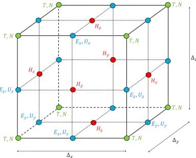
decay of a Langmuir electron plasma wave to an ion-acoustic wave plus a frequency-downshifted Langmuir wave (EDI / LDI); (B) decay of an EM pump wave to a Langmuir wave and an ion-acoustic wave (PDI); (C) decay of an EM pump wave to a frequency-downshifted EM wave plus an ion-acoustic wave (SBS); (D) decay of an EM pump wave to a pair of plasma waves propagating in opposite directions (TPD). Image credit: [Chen, 1984] . . . 61 2.1 Schematic diagram of the fundamental Yee cell [Yee, 1966]. E-field and
H-field component nodes are offset in both space and time, enabling the simulation to be advanced in time using a leapfrog-style update algorithm. 68 2.2 Variation of numerical phase velocity ˜cp with the number of grid cells per
wavelength λ0/∆x for the case of a plane wave propagating along one of the principle gird axes. As the Courant number is reduced, the magnitude of the numerical dispersion error can be seen to increase, particularly at low resolutions. . . 79 2.3 Variation in numerical phase velocity error with wave propagation angle,
for a range of grid resolutions. The Courant ratio was fixed at Sc= 0.5. The ideal case of ˜cp =c is indicated by a dotted line. . . 80 2.4 Variation in numerical phase velocity error with wave propagation angle,
for a range of Courant ratios. The resolution was fixed at ∆x = λ0/16. The ideal case of ˜cp = c is indicated by a dotted line. For cases where Sc > 1/
√
2, the numerical phase velocity is superluminal at some or all propagation angles. . . 81 2.5 Comparison between 1st-order (red) and 2nd-order (blue) Mur-style ABCs
when a Gaussian pulse signal is incident from the left, for the case of Sc=1/
√
3. . . 88 3.1 The basic computational grid unit cell, with the positions of field nodes
3.2 Dispersion curves (upper) and relative errors when compared to the continuous-world regime (lower) for a range of dimensionless parameter ωp4t shown for the ordinary mode (left) and extraordinary mode (right) branches of (3.25). Positive root shown only. Image reproduced from [Cannon and Honary, 2015] © 2015 IEEE. . . 114 3.3 Dissipation curves (upper) and relative errors when compared to the
continuous-world regime (lower) for a range of dimensionless parame-ter ωp4t shown for the ordinary mode (left) and extraordinary mode (right) branches of (3.25). Positive root shown only. Image reproduced from [Cannon and Honary, 2015] © 2015 IEEE. . . 115 3.4 Variation in code performance with the number of work groups per device
compute unit, for a constant work group size. Image reproduced from [Cannon and Honary, 2015] ©2015 IEEE. . . 118 3.5 Variation in code performance with the number of wavefronts in a work
group, for a constant total number of work groups. Image reproduced from [Cannon and Honary, 2015] © 2015 IEEE. . . 119 3.6 Code performance for varying offsets of the z-direction work item index.
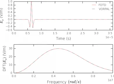
Offset multiples of 32 correspond to coalesced memory access. Image reproduced from [Cannon and Honary, 2015] © 2015 IEEE.. . . 120 3.7 Exsignal for an EM pulse of form (3.29) propagating through a free-space
simulation, recorded at a point 128 cells from the z = 0 launch plane. Upper panel shows time domain comparison of signals measured using the FDTD algorithm described in this work (red) and an equivalent VORPAL simulation (black). Lower panel shows the frequency domain form of the signals, which peak at ωpeak = 4.55×10⁶rad s−1. Computational grid parameters of ∆t= 1.939×10⁻⁸sand ∆x = 11.626m were used in these simulations. Image reproduced from [Cannon and Honary, 2015] © 2015 IEEE. . . 123 3.8 Time domain Ex signal for pulse propagating through an unmagnetised
plasma simulation. Upper panel shows FDTD signal (red), VORPAL signal (blue) and the expected result from plasma theory (black). Central panel shows the error between the simulated signals and the predictions of plasma theory. Lower panel shows the error between FDTD and VORPAL signals. Computational grid parameters of ∆t= 1.939×10⁻⁸sand ∆x= 11.626mwere used in these simulations. Image reproduced from [Cannon and Honary, 2015] © 2015 IEEE. . . 124 3.9 Frequency domain Ex signal for pulse propagating through an
3.10 Time domainExsignal for pulse propagating through a magnetised plasma simulation. Upper panel shows FDTD signal (red) and VORPAL signal (blue). Lower panel shows the error between FDTD and VORPAL signals. Computational grid parameters of ∆t= 1.939×10⁻⁸sand ∆x= 11.626m were used in these simulations. Image reproduced from [Cannon and Honary, 2015] © 2015 IEEE. . . 127 3.11 Frequency domain Ex signal for pulse propagating through a
magne-tised plasma simulation. Upper panel shows discrete Fourier transform of FDTD signal (red) and VORPAL signal (blue). Clear cutoffs can be seen due to the different propagation characteristics of the right- and left-hand circularly polarised components. The expected positions of the cutoffs are indicated in black. Lower panel shows the error between FDTD and VORPAL signals. Computational grid parameters ∆t = 1.939×10⁻⁸s and ∆x = 11.626m were used in these simulations. Image reproduced
from [Cannon and Honary, 2015] © 2015 IEEE. . . 128 3.12 Upper panel shows the numerical refractive index curves for a magnetised
plasma of density profile (3.33). Lower panel shows a comparison of the time averaged O- and X-mode E-field amplitudes measured along the central axis of the computational domain. Computational grid parameters ∆t = 1.939×10⁻⁸s and ∆x = 11.626m were used in the O-mode and X-mode propagation simulations. Image reproduced from [Cannon and Honary, 2015] © 2015 IEEE. . . 130 3.13 Comparison between standing wave pattern developed in FDTD
simula-tion and theoretical calculasimula-tion following the method of [Lundborg and Thid´e, 1986]. Computational grid parameters ∆t = 1.939×10⁻⁸s and ∆x= 11.626m were used in the simulation of the O-mode E-field stand-ing wave pattern. Image reproduced from [Cannon and Honary, 2015] © 2015 IEEE. . . 131 4.1 Angular dependence of O-mode to Z-mode conversion for linear vertical
4.2 Simulated Z-mode window for varying horizontal slope scale sizeLx when background density profile (4.9) is used as a background density profile (smaller Lx implies a steeper slope). It can be seen that increasing the steepness of the slope shifts the centre of the radio window away from the Spitze direction and towards the magnetic zenith. This effect is most pronounced in the case of the 20km curve (the steepest horizontal gra-dient considered here), with no radio window peak seen in the range of angles between vertical (0◦) and field-aligned (12◦); from the shape of the curve, it appears likely that the peak in this case occurs just beyond the zenith direction. The background plasma density, magnetic field direction (dashed line), vertical direction (dotted line) and position of the O-mode reflection height (solid black line) used for each Lx are shown in upper panels. . . 148 4.3 Simulated Z-mode window for varying duct width Lwidth when density
perturbation of (4.10) is included in the background density profile. Initial amplitude of perturbation was set as 5% of the unperturbed background density given by (4.7). Smaller-width structures withLwidth ≤0.1km can be seen to shift the distribution away from the Spitze direction towards vertical by (0.5−1)◦. As the irregularity width increases, the window broadens and loses its Gaussian shape. For widths≥0.2km, a significant fraction of incident wave amplitude was transmitted at all sampled an-gles, leading to a dramatic widening and flattening of the window. The background plasma density, magnetic field direction (dashed line), verti-cal direction (dotted line) and position of the O-mode reflection height (solid black line) used for eachLwidthare shown in upper panels. Compu-tational grid parameters ∆t = 9.17×10⁻⁹s and ∆x = 5.50m were used in these simulations. . . 151 4.4 Time-averaged E-field amplitude for pump wave inclination angles of 0.6◦,
4.5 Time-averaged E-field amplitude for pump wave inclination angles of 0.6◦, 2.9◦, 5.2◦, 7.4◦, 9.7◦and 12.0◦ when periodic density perturbations of the form (4.11) and with Lwidths of 0.08, 0.10, 0.20, 0.50 and 0.80km are included in the background density profile. The position of the X = 1 O-mode reflection contour is marked by a solid line. The colour range has been scaled to more clearly show the transmitted and scattered Z-mode waves beyond the O-Z-mode reflection height. Upper panels show the background electron density, position of the O-mode reflection layer (solid black line), magnetic field direction (dashed black line) and vertical direction (dotted black line) for each Lwidth condition. Computational grid parameters ∆t= 9.17×10⁻⁹sand ∆x = 5.50m were used in these simulations. . . 156 4.6 Upper panels show comparison of the E-field amplitude averaged over
1×10⁵ time steps (9.17×10⁻⁴s) for the case that the upwards boundary of the computational domain is terminated with an absorbing PML (blue) or a reflecting layer (red-dashed). Traces are shown for a selection of initial pump wave inclination angles. Lowermost panel shows the variation of maximum averaged E-field amplitude with inclination angle. It can be seen that allowing the Z-mode wave to reflect enhances the amplification of E-field around the interaction region, particularly for waves directed towards the centre of the radio window around 5.5◦. Computational grid parameters ∆t = 9.17×10⁻⁹s and ∆x = 5.50m were used in these simulations. The critical density for reflection of O-mode waves zc was set to occur 4.1kmabove the lower edge of the computational domain. . . 157 4.7 Change in the simulated E-field amplitude, electron density perturbation
(expressed as a fraction of the background densityNe0), density irregular-ity amplitude (Ne− hNeix)/Ne0, and electron temperature perturbation with time, when Z-mode reflection was suppressed. Spatial snapshots of each quantity are shown for times 1.83×10⁻⁴s, 1.83×10⁻²s, 9.17×10⁻²s, 1.83×10⁻¹s, 2.93×10⁻¹sand 1.10s. Background conditions are shown in the uppermost panel. Computational grid parameters ∆t= 1.83×10⁻⁸s and ∆x = 11.0m were used in this simulation. Field-aligned density irregularities with scale-sizes of approximately 30−40m (∼ 3−4 ∆x) perpendicular to the geomagnetic field can be seen to grow with time around the upper-hybrid resonance height. . . 160 4.8 Change in the simulated E-field amplitude, electron density perturbation
4.9 Variation of electron density and electron temperature perturbation with pump wave inclination angle, for the cases that Z-mode reflection is al-lowed and Z-mode reflection is suppressed. In the reflection-alal-lowed sce-nario, the strongest electron temperature enhancement was found to occur for the pump wave inclined an angle of 5.2◦ (close to the Spitze angle), supporting the argument that the pump wave that is most effectively con-verted the Z-mode excites the greatest temperature perturbation. In the reflection-suppressed scenario, the wave launched in a near-vertical di-rection produced the greatest temperature enhancement. The lowermost panels show the variation of the maximum value of electron temperature enhancement and electron density depletion in the simulation domain with time, for the Z-mode reflection allowed (solid lines) and suppressed (dashed lines) scenarios. Background conditions are shown in the up-permost panel. Computational grid parameters ∆t = 1.83×10⁻⁸s and ∆x= 11.0m were used in these simulations. . . 166 4.10 Right-hand three columns show the simulated growth of small-scale
field-aligned density irregularities with time in a narrow band of altitude be-low the UH resonance level for pump waves directed along 0.0◦, 5.2◦ and 8.6◦ to the vertical. The UH resonance height is indicated by a dashed line. Panels in the leftmost column show the 1D spatial discrete Fourier transform (DFT) ofδN/Ne0 sampled along the horizontal axis of the sim-ulation domain at the height at which the irregularities begin to develop (∼ 2.8km above the lower boundary of the simulation). Amplitude of spatial frequency components around this value increases with time cor-responding to the growth of irregularities and is greater by a factor of 2 or more in the case of the 5.2◦-directed wave. Computational grid param-eters ∆t= 1.83×10⁻⁸sand ∆x= 11.0m were used in these simulations. 168 4.11 Variation in electron density perturbation and electron temperature
per-turbation with pump wave inclination angle when horizontal density slopes of the form (4.9) with Lx = 20km and Lx = 50km were included in the background density profile. Uppermost panels show the background con-ditions for eachLxcase. Lowermost panels show the variation of minimum density perturbation and maximum temperature perturbation recorded in the simulation with time for Lx = 20km (solid line) and Lx = 50km (dashed line). The inclination angle responsible for the greatest temper-ature enhancement shifts from the Spitze position towards the magnetic zenith direction with decreasing Lx, consistent with the modification of the Z-mode window simulated in Section 4.3 (shown in Figure 4.2). Com-putational grid parameters ∆t = 1.22×10⁻⁸s and ∆x = 7.33m were used in these simulations. . . 171 4.12 Variation in electron density perturbation and electron temperature
4.13 Variation in electron density perturbation and electron temperature per-turbation with pump wave inclination angle when periodic density-depleted field-aligned irregularities of the form (4.11) with Lwidth = 0.08km and Lwidth = 0.8km were included in the background density profile. Upper-most panels show the background conditions for each Lwidth. Lowermost panels show the variation of minimum density perturbation and maxi-mum temperature perturbation recorded in the simulation with time, for Lwidth = 0.08km (solid line) andLwidth = 0.8km(dashed line). Compu-tational grid parameters ∆t = 1.22×10⁻⁸s and ∆x = 7.33m were used in these simulations. . . 174 5.1 Variation of background electron plasma frequency (red) and background
electron temperature (blue) with vertical distance from lower edge of the computation domain. From left to right these represent the profiles used in the case of simulated pump wave frequency in the ranges ω0 = (2− 3)ωce,ω0 = (3−4)ωce, andω0 = (4−5)ωce respectively. The points where the electron plasma frequency matches one of the electron gyroharmonics are indicated by ’x’ symbols. . . 194 5.2 Evolution of density perturbation with time for the case of an O-mode
pump wave with frequency ω0 = 4.8ωce. Top panel shows spatial vari-ation of ωpe and ωU H with altitude in the simulation domain. Lower panels show density perturbation snap-shots at various simulation times (increasing downwards). Large-amplitude density depletion can be seen at the O-mode reflection height. Below this, several populations of small-scale density irregularities can be seen to emerge and grow with time, particularly whenωpeandωU H approach an electron gyroharmonic. Com-putational grid parameters ∆t = 1.51×10⁻⁸s, ∆x = 8.82m were used in this simulation. The particularly clear irregularities which form just above ωpe= 3ωce have horizontal spatial scales in the range∼20−40m (∼3−5∆x). . . 196 5.3 Evolution of density perturbation with time for the case of an X-mode
5.4 Examples of the density perturbations developed in the simulation us-ing pump wave frequencies in the range (2−3)ωce. For each frequency, the upper panel displays the spatial snapshot of the electron density per-turbation developed after 0.75s. Note that the colour-map has been logarithmically-normalised. The gyroharmonic heights are indicated by dotted lines. The lower panel for each frequency shows horizontally-averaged vertical profiles of the density perturbation for a range of heights (solid lines). The horizontally-averaged profile from the corresponding O-mode simulation is indicated by the dotted line (recorded after 0.75s simulated time). Computational grid parameters used in these simula-tions can be found in Table 5.1. . . 201 5.5 Examples of the density perturbations developed in the simulation
us-ing pump wave frequencies in the range (3−4)ωce. For each frequency, the upper panel displays the spatial snapshot of the electron density per-turbation developed after 0.72s. Note that the colour-map has been logarithmically-normalised. The gyroharmonic heights are indicated by dotted lines. The lower panel for each frequency shows horizontally-averaged vertical profiles of the density perturbation for a range of heights (solid lines). The horizontally-averaged profile from the corresponding O-mode simulation is indicated by the dotted line (recorded after 0.72s simulated time). Computational grid parameters used in these simula-tions can be found in Table 5.1. . . 203 5.6 Examples of the density perturbations developed in the simulation
us-ing pump wave frequencies in the range (4−5)ωce. For each frequency, the upper panel displays the spatial snapshot of the electron density per-turbation developed after 0.56, s. Note that the colour-map has been logarithmically-normalised. The gyroharmonic heights are indicated by dotted lines. The lower panel for each frequency shows horizontally-averaged vertical profiles of the density perturbation for a range of heights (solid lines). The horizontally-averaged profile from the corresponding O-mode simulation is indicated by the dotted line (recorded after 0.56, s simulated time). Computational grid parameters used in these simula-tions can be found in Table 5.1. . . 205 5.7 Comparison of the electron density perturbation simulated after 0.4sfor
5.8 Top panel shows an example of the anomalous absorption asymmetry for pump wave frequencies ω0 ' 3ωce measured at EISCAT (plot adapted from the upper panel in Figure 10 of [Stubbe et al., 1994]). Central panel shows the variation of the mean-squared irregularity amplitude
h|δN|2i/N02 with ωpe close to the third gyroharmonic height, sampled at similar frequency steps to those used in the upper panel. Bottom panel shows the temporal evolution of h|δN|2i/N02, averaged over the altitude rangezc≥z≥zc−2km. The greatest irregularity amplitude, and hence the greatest expected anomalous absorption, can be seen to occur for 3.1ωce. Computational grid parameters used in these simulations can be found in Table 5.1. Image credit (upper panel): [Stubbe et al., 1994]. . . . 209 5.9 Comparison of the electron temperature perturbations developed in the
simulation domain with and without the inclusion of estimated E-fields due to excited density irregularities in the electron temperature update calculation. Spatial snap-shots of temperature perturbation with and without EES are shown for example pump wave frequenciesω0 = 3.8ωce, ω0 = 4.2ωce andω0 = 4.8ωce(from top to bottom respectively). The gyro-harmonic heights are indicated by dotted lines. The more coarsely-dashed line indicates the X-mode reflection layer for each case. Computational grid parameters used in these simulations can be found in Table 5.1. . . . 215 6.1 The simulated Ek amplitude around the X-mode reflection height for
each set of experimental conditions, averaged over 2 × 10⁵ timesteps (∼2.67ms). The field amplitude corresponding to 3% of the pump wave ERP is indicated by a dashed line for the cases of the 19 October 2012 and 22 October 2013 experiments. For the remaining experiment, the PDI threshold corresponded to ∼ 50% of EPR and therefore was much higher than the maximum simulated E-field amplitude shown here. . . 230 6.2 The variation of maximum simulatedEk amplitudes with irregularity
per-pendicular scale-size when field-aligned density depletions with amplitude 5% of background density were included in the simulation. Results are shown for the pump wave conditions of 22 October 2013 (blue), 19 Octo-ber 2012 (red) and 8 March 2010 (black). For the cases of the 19 OctoOcto-ber 2012 and 22 October 2013 experiments, the maximum simulated Ek for
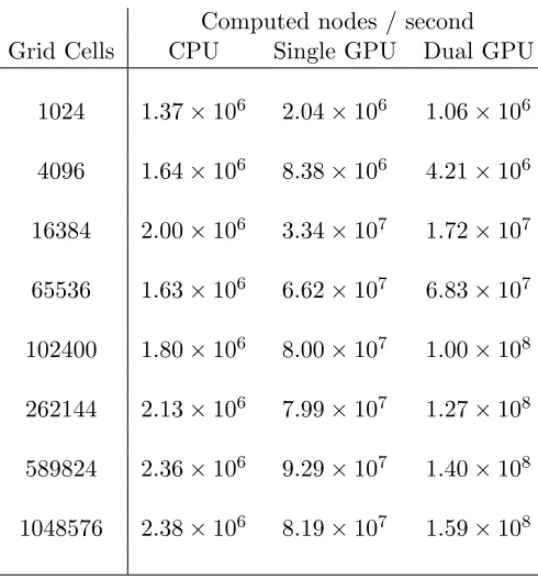
1.1 Parameters typical to the daytime ionosphere . . . 53 3.1 Table comparing the performance of a serial implementation of the FDTD
code running on a single CPU with parallel implementations running on a single GPU and on two networked GPUs. Table reproduced from [Cannon and Honary, 2015] © 2015 IEEE. . . 121 5.1 List of computational grid parameters used for each simulated pump wave
frequencyω0. . . 192
ABC Absorbing Boundary Condition
ADI Alternating-DirectionImplicit
BUM Broad UpshiftedMaximum
CPU Central Processing Unit
CFL CourantFriedrichsLewy
DFT DiscreteFourier Transform
DM Downshifted Maximum
EDI Electron Decay Instability
EM Electromagnetic
ES Electrostatic
FDTD Finite-Difference Time-Domain
FFT FastFourierTransform
GPU GraphicalProcessing Unit
LDI LangmuirDecayInstability
LH LowerHybrid
MZE MagneticZenithEffect
PDI ParametricDecayInstability
PIC Particle-in-Cell
PML Perfectly-MatchedLayer
OTSI OscillatingTwo-StreamInstability
SBS StimulatedBrillouinScattering
SFI Self-Focusing Instability
TPD Two-PlasmonDecay
UH Upper Hybrid
UHR Upper HybridResonance
Introduction: Plasma Physics and
the Ionosphere
Plasma can be defined as a gas in which a fraction of the constituent molecules have non-zero electrical charges. Typically consisting of large numbers of electrons and ionised atoms or molecules moving freely against a background of neutral, un-ionised gas par-ticles, plasmas occur naturally when a neutral gas is subjected to extreme conditions; plasma can be created through raising the temperature of a gas sufficiently high such that increased thermal motion of particles causes collisional ionisation, by bombarding a gas with energetic particles, by illuminating a gas with high-frequency UV or X-ray radiation, or via any other process that can strip electrons from the constituent parti-cles to leave a partially- or fully-ionised gaseous state. Unlike a neutral gas, charged plasma particles can interact with each other through their mutual Coulomb force and will respond to external electrical stimuli such as applied magnetic fields or incident electromagnetic radiation. As such, the dynamical behaviour of even a weakly-ionoised plasma is determined by these electric and electromagnetic interactions, resulting in a diverse range of complicated and collective behaviour not found in neutral gases. The particles in a plasma must beunbound: thermal kinetic energy must dominate over elec-tric potential energy, allowing the plasma to conduct and sustain elecelec-trical currents, and redistribute in response to external electrical stimuli. Several other criteria that must
be met for an ionised gas to be considered a plasma are outlined in Section 1.1 below. Despite the relatively extreme circumstances required for their formation, plasmas make up 99% of all observable matter in the Universe and form a crucial component of almost every aspect of space physics.
This Chapter introduces the fundamental plasma physics principles that form the basis of the numerical simulation code and research studies presented in Chapters 3-6 of this thesis. The structure of the ionosphere and several important observations made by iono-spheric modification experiments are also reviewed briefly below. The descriptions and derivations in this Chapter draw from number of source textbooks, primarily [Baumjo-hann and Treumann, 1996], [Chen, 1984], [Inan and Golkowski, 2011], [Kelley, 1989] and [Kivelson and Russell, 1995]; further detail on any of the topics discussed here can be found within these reference texts.
1.1
Plasma Fundamentals
In this section, the basic properties and collective dynamics of a plasma are derived from simple theory, and the conditions that distinguish a plasma as a specific class of ionised gas, as defined by [Baumjohann and Treumann, 1996], are outlined.
1.1.1 Quasi-neutrality and the Debye Length
perturbations. In response to an applied electric field, the plasma particles will naturally redistribute in order to shield as much of the bulk plasma as possible from the effects of the field. This collective response to external disturbances is known as Debye Shielding
and is an intrinsic and important property of all plasma.
Consider a quasineutral plasma consisting of electrons with number densityNe at equi-librium with singly-ionised positive ions with number density Ni. The quasineutrality condition dictates that Ne ' Ni ' N0. A stationary test point-charge Q located at the origin of a spherically-symmetric coordinate system would induce an electrostatic potentialφat a radial distance r given by:
φ= Q 4πε0r
(1.1)
Over time, the constituent plasma particles will rearrange to form a new equilibrium distribution which takes into consideration the perturbing presence of the test charge. In this simple model, electron motion is assumed to be sufficiently fast compared to the ion motion such that the ions can be considered to be stationary; the plasma can be described by a population of fast-moving electrons immersed in a neutralising bath of static ions. When the plasma has established thermal equilibrium in the presence of applied potential φ, the ion density is thus unchanged and the perturbed electron number density can be expressed using a Boltzmann distribution:
Ne(r) =N0exp
eφ(r) kBTe
(1.2)
where e is the fundamental electric charge, Te is the electron temperature and kB is Boltzmann’s constant. The new potential due to the rearranged particle distribution can be evaluated using Poisson’s equation:
∇2φ(r) =−ρ
ε0
=−Ni−Ne
ε0
where ρ is the charge density. In spherically-symmetric coordinates, (1.3) can be ex-pressed as:
1 r2
d dr
r2 d
drφ
=−1
ε0
eN0−eN0exp
eφ(r) kBTe
' −eN0
ε0
1−
1 +eφ(r) kBTe
' e
2N 0
ε0kBTe
φ(r) (1.4)
Solving this differential equation forr >0 results in the solution:
φ(r) =φ0(r) exp
− r
λD
(1.5)
where φ0(r) is the potential from the perturbing test charge as shown by (1.1) and λD is the Debye shielding length:
λD =
ε0kBTe N0e2
12
(1.6)
The collective response of the plasma to the perturbation is therefore to rearrange such that the potential due to the test charge is exponentially attenuated with distance. At short distances from the charge (r → 0) the potential tends to that of the unshielded test charge (φ(r)→φ0(r)). As the distance from the charge increases, the potential falls more rapidly than the free-space Coulomb potential, until at long distances (r λD) the test charge is effectively completely shielded (φ(r)→0). Thus, the Coulomb force due to the test charge is able to extend only∼λD into the plasma. As the electron temperature increases, λD increases as electrons have a greater thermal kinetic energy and can more easily resist the attractive / repulsive effect of the test charge. λD decreases as plasma density increases as there are more particles available to contribute to the shielding process. In a more realistic case, where the ions are not static, the Te term in (1.6) is replaced by an effective temperature Te+Ti.
the plasmaLmust be much greater than the Debye scale (LλD) otherwise shielding cannot take place and quasineutrality cannot be established.
1.1.2 Plasma Parameter
The shielding of excess charge in plasma takes place over radial distance scaleλD, in a volume known as theDebye Sphere. The number of particles of a single species involved in the shielding process,nD, can be expressed as:
nD ' 4 3πλ
3
DN0 (1.7)
where N0 is the unperturbed density of electrons or ions. This allows the plasma
pa-rameter, Λ, to be defined as:
Λ≡N0λ3D (1.8)
Substituting the definition ofλD, (1.6):
Λ∝ (kBTe)
3/2
N01/2 (1.9)
In a plasma, the constituent particles must be unbound and free to move. For this to be the case, the thermal kinetic energy of the particles (∝ kBT) must dominate over the Coulomb potential energy (∝interparticle distance, N0−1/3). Thus the plasma parameter can be used to define a second key condition for an ionised gas to be considered a plasma [Baumjohann and Treumann, 1996]:
Λ =N0λ3D 1 (1.10)
1.1.3 Cold Plasma Oscillation
In the simplified model of cold plasma described above, low-mass, fast electrons move against a background of heavy, slow ions. In response to an external force, the electrons will be displaced while the position of the ions will remain relatively unchanged; the mu-tual attraction between the stationary ions and displaced electrons provides the restoring force in a simple harmonic oscillator system, in which the displacement of plasma elec-trons fluctuates periodically around an equilibrium position with a frequency defined by the plasma conditions. The periodic oscillation of plasma particles in response to an applied electric field is a fundamental property of a plasma: the plasma frequency. To demonstrate this, consider an isolated block of cold plasma of dimensions L×L×L, at equilibrium at time t = 0, shown schematically in Figure 1.1 (a). If an externally-applied force was to suddenly displace all electrons from their equilibrium positions by a distance +x, this would leave an excess charge of +eN0L2xon one edge of the plasma due to all the stationary ions left behind, as shown in 1.1 (b). From Gauss’s Law, the E-field between the displaced electrons and the un-moved ions is given by:
I
S
E·dS= 1 ε0
Qenclosed
where surfaceS surrounds the volume of excess positive charge.
⇒ExL2 =
eN0L2x
ε0
Ex = eN0
ε0
x (1.11)
The force exerted on the electrons due to this induced E-field is given by:
F =me d2x
dx2 =−eEx
⇒ d
2x
dx2 =−
e2Ne ε0me
x (1.12)
ex ces s p o sitiv e cha rg e 𝐸𝑥 ex ces s n egative cha rg e 𝐸𝑥 electron acceleration + + + + + + + + + + + + + + + + + + + + + -- -- -+ + + + + + + + + + + + + + + + + + + + + -- --
-electrons displaced by distance 𝑥
quasineutral plasma of electrons and positive ions
L 𝑥 excess p o siti ve ch ar ge ex ces s n egative cha rg e 𝐸𝑥 𝐸𝑥 electron acceleration
(a)
(b)
+ + + + + + + + + + + + + + + + + + + + + -- ---electrons accelerated by restoring force from ion attraction
(c)
leads to simple harmonic oscillation of electrons around equilibrium positions
[image:28.596.123.493.134.651.2]𝑥
Figure 1.1: Schematic diagram of the fundamental cold plasma oscillation in response
can be expressed as a function of the plasma density:
ωpe =
e2Ne ε0me
12
(1.13)
In reality, the ions are unlikely to be completely motionless, and will oscillate around their equilibrium position in response to an applied E-field with frequencyωpi:
ωpi=
Z2 ie2Ni ε0mi
12
(1.14)
where Ze is the total charge on the ionised particle. This leads to a to an overall fundamental frequency of plasma oscillation given by:
ω2p =ωpe2 + X ion species
ωpi2 (1.15)
Due to the significant mass difference between electrons and ions,memi, the electron plasma frequency usually dominates the ion plasma frequency, meaning that ωp ' ωpe under most conditions.
Any perturbation to a cold plasma resulting in small displacements of the plasma par-ticles from their displacement positions; for example, the effect of a propagating radio wave will cause the plasma to oscillate at a frequency entirely determined by the local plasma properties. Most plasmas are only partially-ionised, with the charged species moving against a background of un-ionised neutral particles: plasma oscillations can only be sustained if the collision rate between electrons and neutrals, νen, is sufficiently small compared to the plasma oscillation frequency. From this, a third criterion re-quired for an ionised gas to be classified as a plasma can be defined [Baumjohann and Treumann, 1996]:
ωp νen
1 (1.16)
the case of imperfectly-ionised, collisional plasmas.
From the definition of the Debye length:
λD =
ε0kBTe N0e2
12
=
kBTe me
12
1 ωpe
' vT e
ωpe
(1.17)
where vT e is the electron thermal velocity. The Debye length can be defined as ap-proximately the distance an electron can travel via thermal motion during one plasma oscillation period.
1.2
Single-Particle Motion
Much of the plasma behaviour discussed in this thesis is in the context of the plasma as a fluid; the collective, bulk response of the plasma medium to externally-applied forces or perturbations, such as illumination via high-power electromagnetic waves. The root of this macroscopic behaviour, however, arises from the microscopic dynamics of individual charged particles in the presence of applied electric or magnetic fields. In this Section, the basic motion of a single charged particle due to external applied forces is discussed.
1.2.1 Lorentz Motion and Gyration
The motion of a single non-relativistic particle of charge q and mass m is governed by the Lorentz force:
F=mdv
dt =q(E+v×B) +Fother (1.18) wherevis the particle velocity andFotherbundles together of all the non-electromagnetic forces acting on the particle, for example pressure or gravity.
In the presence of an electric field only (B = 0), the particle simply experiences a constant acceleration qEparallel to the applied E-field. The direction of acceleration is dictated by the polarity of the particle’s charge: positive ions follow the E-field direction; electrons and negative ions travel anti-parallel to the E-field. Under an applied E-field,
In the presence of a magnetic field only (E = 0), the particle is accelerated in a di-rection perpendicular to both B and v. The kinetic energy of the particle will remain unperturbed, as demonstrated by taking the dot-product of v with (1.18) (assuming Fother'0):
mv·dv
dt =qv·(v×B)
⇒ d
dt
1 2m|v|
2
= 0 (1.19)
No work is done on the particle by the applied B-field, and the particle therefore can receive no acceleration along the field direction. Instead, the particle rotates conserva-tively in the plane perpendicular to the B-field, as shown in Figure 1.2; this orbit around Bis known asgyromotion. Assuming an externally-applied B-field along thez-direction, B=Bˆz, the particle acceleration can be expressed as:
mdv dt =m
˙ vx ˙ vy ˙ vz = qBvy
−qBvx 0 (1.20)
Note that vx and vy are π/2 out of phase. Taking the second derivative of (1.20) and substituting in expressions for ˙vx,y yields:
¨ vx ¨ vy ¨ vz = qB mv˙y
−qBmv˙x 0 =
−ω2 cvx
−ωc2vy 0 (1.21)
From this equation it is clear that, provided the particle initially has a non-zero compo-nent of velocity in the plane perpendicular to the B-field, circular motion in this plane will occur with an orbital frequency defined as thegyrofrequency orcyclotron frequency, ωc:
ωc=− q|B|
m (1.22)
𝐵ො𝒛 𝐵ො𝒛
𝑣‖ 𝑦
𝑥
-𝑣⊥ 𝑅𝑐
[image:32.596.121.466.94.308.2]‖
Figure 1.2: Schematic diagram of an electron moving in a uniform, time-invariant
B-field,B=Bˆz. Presence of a magnetic field causes the electron to rotate in a plane perpendicular to the field direction. Motion parallel to the magnetic field combined with simultaneous gyrorotation in the perpendicular plane leads to helical motion of the particle following the field direction. A positive ion would rotate in the opposite
sense to the electron due to their opposing polarities.
pointing towards the observer); positive ions will rotate in the opposite sense. Due to
the large mass difference (me mi), the gyrofrequency for electrons is generally much
greater than for ions (ωce ωci).
1.2.2 Guiding Centre Drift
In the presence of an applied magnetic field, a charged plasma particle will orbit in
the plane perpendicular to the field with frequencyωc, with the parallel component of
velocity unperturbed; non-zero parallel motion combined with simultaneous gyrorotation
in the perpendicular plane leads to helical motion of the particle following the magnetic
field line, as shown in Figure 1.2. In more complex situations, perhaps with the inclusion
of an electric field, or where the magnetic field is not uniform, it is useful to consider the
average motion of the particle’s guiding centre: following the centre of the gyromotion allows the motion of the particle to be followed as if it were time-averaged over several
To illustrate this, consider the case of an time-independent force acting on the particle in addition to a constant B-field. A force aligned with the magnetic field,Fk, will simply
accelerate the particle such that its parallel velocity component can be described by:
dvk
dt = Fk
m (1.23)
⇒vk(t) =vk(0) +
Fk
mt (1.24)
More interesting is a force lying in the plane perpendicular to the magnetic field, F⊥,
which may act such that the position of the guiding centre is not necessarily constant in this plane. In this case, the perpendicular velocity will be described by:
dv⊥
dt =ωc×v⊥+ F⊥
m (1.25)
whereωc=−qB/m. Differentiating (1.25) with respect to time and rearranging yields:
d2v⊥
dt2 =ωc×
dv⊥
dt
=ωc×
ωc×v⊥+
F⊥
m
= −ω2cv⊥
| {z }
gyromotion
+ωc×F⊥ m
| {z }
drift
(1.26)
using ωc×ωc×v⊥ = ωc(ωc·v⊥)−ωc2v⊥ = −ωc2v⊥. The first term is simply the
harmonic gyromotion derived in Section 1.2.1 above. The second term causes the guiding centre of the particle’s rotation to drift in a direction perpendicular to both the force direction and the magnetic field direction, with a constant drift velocity vF⊥:
vF⊥=
ωc×F⊥
mω2 c
=
1 q
F⊥×B
B2 (1.27)
Figure 1.3: Schematic diagram of electron and ion drift motion for the cases of no perpendicular field, a perpendicular E-field and a perpendicular B-field gradient.
(note that this is a cartoon only: the gyroradii are not to scale)
both the applied E-field and applied B-field:
vE⊥ =
1 q
(qE⊥)×B
B2 =
E⊥×B
B2 (1.28)
the particle in the plane of rotation will reduce rc. Over the remaining part of its gyrorotation, the particle moves in the same direction as the E-field and is accelerated, increasing its radius of rotation. The combination of wide loops as the particle moves with the field and tight corners as it moves against the field leads to a net constant drift in the E×B direction. An electron rotates in the opposite sense, but also gains and loses velocity with the field in the opposite direction (accelerates moving against the field, decelerates moving with the field), and thus the drift motion occurs in the same direction as for the positive ion.
An additionalpolarisation drift term emerges when the E-field is allowed to vary slowly with time. In this context,slowly-varyingimplies slow compared to the particle cyclotron frequency. To evaluate this, the cross-product of (1.25) withB/B2 is taken, for the case that perpendicular force F⊥ is a time-dependent E-field perpendicular toB:
dv⊥
dt × B
B2 =ωc×v⊥× B B2 +
qE⊥(t)×B
mB2
Using the expansionωc×v⊥×BB2 =v⊥
ωc·B B2
| {z }
qB
m·
B
B2
−B
B2 (ωc·v⊥)
| {z }
0
=−mqv⊥:
v⊥=
E⊥(t)×B
B2 −
m q
dv⊥
dt × B B2
v⊥=vE−
m qB2
d
dtv⊥×B (1.29)
Averaging over many gyrorotation periods, v⊥×B ' −E⊥. Thus, the slowly-varying
solution can be expressed as:
⇒v⊥=vE + 1 ωcB
dE⊥
dt
| {z }
polarisation drift velocityvP
(1.30)
is proportional to particle mass, and as such is much greater in the case of ions than electrons. The differential motion of electric charges induces a polarisation current,JP, carried mostly by the ions in a electron/positive ion plasma due to the large mass ratio me mi.
JP =eNivP i−eNevP e' N0(mi+me)
B2
dE⊥
dt (1.31)
for a quasineutral plasma with Ni 'Ne'N0.
From the general drift equation (1.27), particle guiding centre velocities can easily be found for any time-invariant applied force using the same technique as above, for example the force due to gravity leads to:
FG=−mg⊥⇒vG=−
1 ωc
g⊥×B
B (1.32)
where g⊥ is the component of gravitational acceleration perpendicular to the applied
B-field. Unlike in the static E-field case, particles of different polarities will drift in different directions and the magnitude of velocity is no longer invariant between particle types.
The above scenarios all assume that the magnetic field is uniform in space. A further class of drifts occur due to inhomogeneities in the magnetic field. Consider a particle in the presence of a weak gradient in the magnetic field, whereweak in this context implies that the scale size of spatial variation of the field is much greater than the particle’s radius of gyrorotation. The variation in the field will cause the radius of gyromotion to change over the course of one orbit, leading to a net drift of the guiding centre, in a similar manner to that described for E×B drift above. This corresponds to a force of the form F∇B =−ΘM∇B acting on the particle, where ΘM =mv⊥2/2B is the magnetic moment of the gyrorotation. Substituting this force into the general drift equation (1.27) yields a particle drift of:
v∇B= mv2⊥
qB3 (∇B)×B (1.33)
the drift plane, 12mv2⊥, as faster particles will experience more of the field variation, as illustrated schematically in Figure 1.3.
A further drift due to B-field inhomogeneity occurs when the field lines are curved. In this case, the particles trying to move along the field line experience a centrifugal force corresponding toFC =mvk2RC/R2
C, whereRC is the radius of curvature. From (1.27) this
leads to a drift of:
vC = mv 2
k
qR2CB2RC×B (1.34)
Again, this drift induces differential motion of electrons and positive ions, and increases in magnitude with kinetic energy along the field line, as particles moving faster in this direction will experience more of the field line curvature.
1.3
Plasma Dynamics
The above Section 1.2.2 describes the motion of a single charged particle under the influence of external stimuli, however to describe the dynamic behaviour of plasma a more collective approach is required. As every pair of particles in a plasma share a mutual interaction, an analytical approach that involves tracking the time-dependent motion of every individual particle is impossible, and numerical computation of the motion of individual particles is far too computationally-intensive to be feasible. To allow the dynamics of a plasma system to be described and modelled, several schemes of approximations can be made; two commonly-used formulations of this nature are described below.
1.3.1 Kinetic Formulation
respectively. The probability of a particle having a particular r and v at time t is de-scribed by the particle distribution functionf(r,v, t). Plasma quantities such as particle count or number density can be evaluated by integrating over this function:
Number of particles: N =
Z Z ∞
−∞
f(r,v, t)drdv (1.35)
Number density: N =
Z ∞
−∞
f(r,v, t)dv (1.36)
There is no restriction on the form of distribution functionf; in the case of cold plasma a delta function is appropriate, while a Maxwellian distribution is often adopted for the case of a warm plasma with non-zero temperature.
To investigate the behaviour of the particle distribution function under the influence of an applied force F, consider an element of phase space with volume dV = drdv, and surface areas in position- and velocity-space dSr and dSv respectively. Assuming conservation of particles, the net flux of particle into the volume in both position- and velocity-space balances the rate of change of particle count within the volume:
d dt
Z
f dV + Z
fv·dSr+ Z
fdv
dt ·dSv = 0 (1.37)
Using the divergence theorem (∇ ·A)dV =A·dS and rearranging gives an expression for thecollisionless Boltzmann equation:
d
dtf drdv+∇r·(fv)drdv+∇v·
fdv dt
drdv= 0
⇒ df
dt + (v· ∇r)f +
F m · ∇v
f = 0 (1.38)
whereF is assumed to be independent ofv,∇r =ˆx∂x∂ +ˆy∂y∂ +ˆz∂z∂ and ∇v =ˆvx∂v∂x +
ˆ
vy∂v∂y+vˆz∂v∂z. In a cold, magnetised plasma, the external force term is provided by the
Lorentz equation to give theVlasov equation:
dfa
dt + (v· ∇r)fa+ ea ma
[(E+v×B)· ∇v]fa= 0 (1.39)
conditions to determine the time dependent, kinetic behaviour of the plasma population. Physical quantities such as density or energy can be deduced taking moments of the distribution function In the case of a collisional plasma, an additional term (∂f/∂t)
coll must be included on the right-hand side of equation (1.39) [Inan and Golkowski, 2011].
1.3.2 Fluid Formulation
The fluid formulation of plasma dynamics follows directly from the kinetic approach: bulk-averaged quantities representing observable parameters such as momentum or en-ergy can be obtained by taking moments of the Vlasov equation (1.39). The fluid average for any parameterA at positionr and timetcan be found via:
A(r, t) =hAi= 1 N(r, t)
Z
A(r, t)f(r,v, t)dv (1.40)
where the number densityN(r, t) is given by (1.35). For example, the plasma bulk-fluid velocity can be expressed as:
U(r, t) =hvi= 1 N(r, t)
Z
v(r, t)f(r,v, t)dv (1.41)
In the multiple-fluid formulation, each plasma species can be represented as a separate fluid. For each component, fluid equations describing the dynamical behaviour of mo-mentum, number density and energy can be found by multiplying the Vlasov equation by these parameters and integrating over velocity space. These can be combined with Maxwell’s equations to give a coupled set of multiple-fluid equations that completely describe the time-dependent evolution of bulk-fluid quantities in an ionospheric plasma, as given by equations (1.42)-(1.48) [Inan and Golkowski, 2011, Gurevich, 1978]:
∇ ·E= 1 ε0
X
a Naea
| {z }
charge densityρ
(1.42)
∇ ·B= 0 (1.43)
−µ0
∂H
ε0
∂E
∂t =∇ ×H− X
a=e,i
NaeaUa
| {z }
current densityJ
(1.45)
Nama
∂Ua
∂t + (Ua· ∇)Ua
=Naea(E+Ua×B)−. . .
· · · −NamaνaUa− ∇(γkBNaTa)
| {z }
pressure gradient∇p
(1.46)
∂Na
∂t +∇ ·(NaUa) = 0 (1.47)
3 2kB
∂
∂t(NaTa) + ∇ ·| {zQa} heat flux transport
=NaeaE·Ua
| {z }
ohmic heating
+ 4εa |{z} collisional
heating
(1.48)
where a =e, i for electrons and ion species, and νa is the effective collision frequency. These equations will form the basis of the plasma-fluid finite-difference time-domain simulation algorithm developed in Chapter 3.
1.4
Waves in Plasma
flavour from a superposition of competing interactions. The need for a way to model the time dependent evolution of many mutually-interacting complicated and often non-linear plasma phenomena is one of the prime motivations behind the development of the time-explicit numerical code described in Chapter 3.
A plasma wave can be described through a medium-dependent dispersion relation, which defines how the wave frequency ω varies with its propagation vector k. To construct a dispersion relation, Maxwell’s Equations (1.42)-(1.45) are converted from the time-domain to the frequency-time-domain assuming plane-wave solutions of the form ei(ωt−k·r) and thus using the Fourier transform pairs ∇ → −ik and∂/∂t→iω to give:
k·ε·E= 0 (1.49)
k·B= 0 (1.50)
k×E=ωB (1.51)
k×B=−ωµ0ε·E (1.52)
In these expressions, the dispersive effects of the plasma have been wrapped up into the dielectric permittivity tensorε, defined such that:
ε·E= 1 iωε0
J+E=
1+ σ iωε0
·E (1.53)
whereσ is the plasma conductivity tensor. Taking the frequency-domain curl of (1.51) and (1.52) and rearranging gives the basic plasma dispersion relation (1.54):
k(k·E)−k2E+
w
c
2
ε·E= 0 (1.54)
whereB= 0. From (1.51), this condition implies that these waves are longitudinal with k×E= 0. The termElectromagnetic (EM) will refer to waves withB6= 0.
1.4.1 Electromagnetic Waves
In a vacuum, an electromagnetic wave travels at a constant speed of light and obeys the simple dispersion relation given by (1.55):
ω2=c2k2 (1.55)
However a plasma acts as a dispersive and often anisotropic medium that can signifi-cantly influence the propagation of the wave. Below, the dispersive behavior for elec-tromagnetic waves under various plasma conditions are summarised, treating the wave fields E and B as small perturbations to the medium. As EM waves require B 6= 0, dispersion relations can be found by using equation (1.54) with the appropriate expres-sion for ε. The derivations outlined below can be found in more detail in [Inan and Golkowski, 2011] and other textbooks.
1.4.1.1 Unmagnetised Plasma
The simplest case of plasma is a uniform, cold, collisionless and unmagnetised combina-tion of electrons and singly-ionised positive ions at thermal equilibrium, as encountered in Section 1.1 above. The oscillating electric field of an EM wave travelling through this plasma will displace the plasma particles from their equilibrium positions, causing them to attempt to oscillate at the plasma frequency as described in Section 1.1.3. The restoring electric field induced by the plasma oscillations interferes with the EM field, introducing frequency-dependent dispersive effects. In the cold, collisionless case with B0 = 0 and νc = 0, the electron momentum equation (1.46) can be expressed in the frequency domain as:
iωUe=− e
me
Assuming that the ions are stationary on the timescale of electron oscillations, the induced current can be described by:
Je =−eNeUe = e 2N
e iωme
E (1.57)
where the unmagnetised and thus isotropic condition implies scalar values for the conduc-tivity and permitconduc-tivity. The EM dispersion relation can be obtained by using equation (1.54) in conjunction with the transverse condition k·E= 0 to give:
c2k2
ω2 E=ε·E or
1−c
2k2
ω2
E=− 1
iωε0
J (1.58)
Finally, substitution of (1.57) into (1.58) gives:
1−c
2k2
ω2
E=− 1
iωε0
e2Ne iωme
E (1.59)
which simplifies to give a dispersion relation for EM waves in a cold unmagnetised plasma:
ω2 =ωpe2 +k2c2 (1.60)
using expression (1.13) for the electron plasma frequency ωpe.
The EM dispersion relation for unmagnetised plasma is plotted in Figure 1.4. From this it is clear an unmagnetised plasma is completely opaque to EM waves with a fre-quency below the characteristic frefre-quency of electron oscillation. This corresponds to a frequency cut-off at ω =ωpe, and a critical value of electron number density, NeCrit,
above which the wave cannot propagate:
NeCrit =
ε0me e2 ω
2
0 (1.61)
As the frequency is increased beyond ωpe, the expression converges to the vacuum dis-persion relation (1.55).
Figure 1.4: Dispersion relation for electromagnetic waves in a cold, collisionless, unmagnetised plasma (red). There is a frequency cut-off at ω = ωpe, below which
there is no wave propagation. The relationship asymptotically approaches theω =ck vacuum expression as frequency is increased (indicated by dashed-black line).
the dispersion relation. With effective collision frequencyνc = 0, the frequency-domain
momentum expression (1.56) becomes:
iω1−iνc
ω
Ue=−
e
me
E (1.62)
Addition of collisions effectively corresponds to the substitutionm→m(1−iνc/ω) [Inan
and Golkowski, 2011]. This leads to the appearance of a frequency-dependent
negative-imaginary damping term in the dispersion relation, which manifests physically as an
exponential attenuation of the wave with distance:
ω2 =ωpe2 +k2c2+iνcω
1−k
2c2
ω2
(1.63)
1.4.1.2 Magnetised Plasma
In this unmagnetised plasma scheme above, the components of the propagating electric
field are uncoupled: propagation is not sensitive to the wave polarisation; dispersive