boundary-driven open quantum chains
Federico Carollo, Juan P. Garrahan, Igor Lesanovsky and Carlos P´erez-Espigares School of Physics and Astronomy and
Centre for the Mathematics and Theoretical Physics of Quantum Non-Equilibrium Systems, University of Nottingham, Nottingham, NG7 2RD, UK
(Dated: October 6, 2017)
We consider a class of either fermionic or bosonic non-interacting open quantum chains driven by dissipative interactions at the boundaries and study the interplay of coherent transport and dissi-pative processes, such as bulk dephasing and diffusion. Starting from the microscopic formulation, we show that the dynamics on large scales can be described in terms of fluctuating hydrodynamics (FH). This is an important simplification as it allows to apply the methods of macroscopic fluc-tuation theory (MFT) to compute the large deviation (LD) statistics of time-integrated currents. In particular, this permits us to show that fermionic open chains display a third-order dynamical phase transition in LD functions. We show that this transition is manifested in a singular change in the structure of trajectories: while typical trajectories are diffusive, rare trajectories associated with atypical currents are ballistic and hyperuniform in their spatial structure. We confirm these results by numerically simulating ensembles of rare trajectories via the cloning method, and by exact numerical diagonalization of the microscopic quantum generator.
I. INTRODUCTION
There is much interest nowadays in understanding the collective macroscopic behaviour of non-equilibrium quantum systems that emerges from their underlying microscopic dynamics. This includes problems of ther-malisation [1–5] and of novel non-ergodic [6] and driven phases [7] in quantum many-body systems, issues which also have started to be addressed experimentally [8–13]. Given that in practice interaction with an environment, while sometimes controllable, is always present, an im-portant question is to what extent the interplay between coherent dynamics and dissipation influences the collec-tive properties of such quantum non-equilibrium systems [14–20].
The hallmark of a driven non-equilibrium system is the presence of currents. Recently there has been impor-tant progress in the description of current bearing quan-tum systems with two complementary approaches. One corresponds to the study of quantum quenches where two halves of a system are prepared initially in differ-ent macroscopic states, and where the successive non-equilibrium evolution displays stationary bulk currents associated with transport of conserved charges [21–26]. Another corresponds to studies of one-dimensional spin chains coupled to dissipative reservoirs at the bound-aries and described by quantum master equations [27– 42]. While the transport depends on the precise nature of the processes present in the system, the studies above find that in appropriate long wavelength and long time limits the dynamics can be described in terms of effec-tive hydrodynamics. A central question is to what extent the non-equilibrium dynamics of systems where there is an interplay between quantum coherent transport and dissipation displays behaviour similar to that of classical driven systems [43].
Here we address the statistics of currents in driven
dis-sipative quantum systems and the spatial structure that is associated with rare current fluctuations. We consider quantum chains for either fermionic or bosonic particles driven dissipatively through their boundaries. We also al-low for dephasing and/or dissipative hopping in the bulk. Previous studies of similar systems have shown that with bulk dephasing and/or dissipative hopping transport is diffusive, while in the absence of both it is ballistic [30– 33]. We show that the large scale dynamics of these sys-tems in general admits a hydrodynamic description in terms of macroscopic fluctuation theory (MFT) [44]. In particular, we show that quantum stochastic trajectories can be described at the macroscopic level in terms of fluctuating hydrodynamics (FH) [45]. This macroscopic dynamics corresponds to that of the classical symmetric simple exclusion (SSEP) for fermionic chains, and to the classical symmetric inclusion processes (SIP) for bosonic chains [46–49].
The effective classical MFT/FH description in turn al-lows us to obtain the large deviation (LD) [50] statistics of time-integrated currents [43, 51, 52]. The cumulant generating function, or LD function, plays the role of a dynamical free-energy, and its analytic structure re-veals the phase behaviour of the dynamics [53–64]. We find that in fermionic open chains the LD function dis-plays a third-order transition between phases with very different transport dynamics. Similar LD criticality was found for classical SSEPs with open boundaries [65, 66]. We show that this transition is manifested in a singular change in the structure of the steady state, from diffu-sive for dynamics with typical currents, to ballistic and
II. MODELS AND EFFECTIVE HYDRODYNAMICS
We consider a class of one-dimensional bosonic or fermionic non-interacting quantum systems of L sites, weakly coupled to an environment, and connected at its first and last sites to density reservoirs. In the Markovian regime, we assume the evolution of a system operatorX to obey the following Lindblad equation [68, 69],
∂tXt=i[H, Xt] +D∗[Xt], (1) whereH is a quadratic Hamiltonian
H = M X
h=1
Jh L−h X
k=1
a†k+hak+a†kak+h
, (2)
witha†k, ak denoting (bosonic or fermionic) creation and annihilation operators acting on site k. Here Jh is the coherent hopping rate between a given site k and the sites k±h. The largest hopping distanceM is assumed to be finite and independent of L, with M = 1 corre-sponding to only nearest-neighboring hops. The super-operator D(·) := P
µVµ(·)Vµ† − 1 2{V
†
µVµ,(·)} is a Lind-blad dissipator modelling the coupling to the environ-ment; Vµ are jump operators, and {·,·} stands for the anticommutator. The dissipator has three contributions,
D := D1+DL +Dbulk. The first two corresponds to boundary driving terms where particles are introduced at site 1 and L with ratesγin
1,L and removed with rates γout
1,L, cf. [35, 36],
D∗1,L[X] :=γ1in,L
a1,LXa†1,L− 1 2{a1,La
†
1,L, X}
+
+γ1out,L
a†1,LXa1,L− 1 2{a
†
1,La1,L, X}
. (3) The third contribution accounts for dissipation in the bulk, including site dissipation with rateγand dissipative hopping with rateϕ, cf. [32, 33],
D∗bulk[X] :=γ L X
k=1
nkXnk− 1 2{n
2 k, X}
+ (4)
+ϕ 2
L−1 X
k=1
[[L†k, X], Lk] + [[Lk, X], L†k]
,
with nk =a†kak being thek-th site particle number op-erator, andLk =a†k+1ak.
To derive the effective macroscopic description we con-sider the average occupation on each site hnmit, which from Eqs. (1-4) obeys acontinuity equation,
∂thnmit=−h M X
h=1
jh,mco −j co h,m−h
+ jmdis−j dis m−1
it, (5)
where jco
h,m := −i Jh(a †
m+ham−a †
mam+h), and jmdis := ϕ(nm−nm+1), are the different current contributions:
jh,mco is the coherent, and thus quantum in origin, par-ticle current between sites m and m+h, while jdis
m is the analogous of the stochasticcurrent in SSEPs. The next step is to rescale space and time by suitable pow-ers of the chain lengthLto get meaningful equations in the thermodynamic limit. The correct rescaling is the diffusive one, in which the macroscopic space and time variables are given byx:=m/L∈[0,1], and τ :=t/L2. In the new time-coordinate, the evolution of the average occupation number is implemented by
∂τhnmiτ =−L2h M X
h=1
jh,mco −jcoh,m−h
+ jmdis−jmdis−1 iτ.
(6) In order to derive an equation for the average density one needs to focus on the quantum current jh,mco , and to understand what is its contribution in the diffusive scaling. Neglecting terms which are not contributing in the rescaled space-time framework, (see Appendix A for a detailed discussion on the hydrodynamic limit), one has the following time-derivative for the current
∂τhjh,mco iτ≈L2 h
2Jh2hnm−nm+hiτ−˜γhjh,mco iτ i
, (7) where ˜γ =γ+ 2ϕ >0 is the total dephasing rate. For-mally integrating the above equation, neglecting expo-nentially decaying terms, one has
hjh,mco iτ ≈2Jh2L 2Z
τ
0
due−γL˜ 2(τ−u)hnm−nm+hiu;
for very largeL,L2e−γL˜ 2(τ−u)converges, under integra-tion, to a Dirac delta, (see Eq. (A1) in Appendix A), and thus the quantum contributions to the current become
hjh,mco iτ ≈ 2J2
h
γ+2ϕhnm−nm+hiτ. Substituting this into (6), and recasting the various contributions, one finds
∂τhnmiτ ≈ϕL2hnm+1−2nm+nm−1iτ+ +2L
2
˜ γ
M X
h=1
Jh2hnm+h−2nm+nm−hiτ. (8)
The above expectations are proportional to finite-difference second-order derivatives. This means that when introducing the macroscopic density ρτ(x) :=
hnm=xLit=τ L2, defined on the rescaled macroscopic
space, in the largeLlimit, one obtains the hydrodynamic equation
∂τρτ(x) =D ∂2xρτ(x), (9) where the effective diffusion rate reads
D:= ϕ+ 2 γ+ 2ϕ
M X
h=1
Jh2h2
!
. (10)
allτ (see Appendix A), %0:=
γin 1
γout 1 ±γ1in
, %1:=
γin L γout
L ±γLin
, (11) where plus is for fermionic systems, while the minus, re-stricted to the case γ1out,L−γ1in,L>0, is for bosonic ones. Such restriction is necessary in the bosonic case in or-der to achieve a convergence of the boundary conditions. Equations (9), (10) and (11) encode the diffusive hydro-dynamics of both fermionic and bosonic chains governed by Eq. (1). This result agrees with previously studied special cases: for example, in the tight-binding (M = 1) fermionic case without dissipative hopping, Eq. (7) re-duces to the diffusive rate of [36], while for dissipative hopping without dephasing to the one found in [33]. The macroscopic dynamics Eqs. (9-11), thus unifies previ-ous findings and predicts the behaviour for more general Hamiltonians, including also the bosonic case. For non-quadratic Hamiltonians (interacting systems), our proce-dure cannot be directly applied as it is not straightfor-ward to close the differential equations for the densities in the hydrodynamic limit. However, for particular lim-iting cases, it is possible to make predictions on how mi-croscopic interactions modify the hydrodynamic behavior of the system through a diffusion rate which in general depends on the density profile. In the next section we discuss one of these cases.
III. EXAMPLE OF HAMILTONIAN WITH INTERACTIONS
We consider a fermionic system whose bulk dynamics is implemented by
∂tX =i[HInt, X] +γ L X
k=1
nkXnk− 1
2{nk, X}
,
where the Hamiltonian, HInt =H+HV has also an in-teraction term
H =J L−1 X
k=1
a†k+1ak+a†kak+1
, HV =V L−1 X
k=1
nknk+1.
The driving at the chain’s ends is treated in the same way as in the previous section, providing the same density at the boundaries in terms of the injection and removal rates (11). We are interested in deriving a hydrodynamic equa-tion for the above system in the limit of strong dephas-ing and strong interaction, i.e.|V|, γ |J|, as well as in shedding light on the role played by interactions in the coarse-grained description. To this aim it proves conve-nient to introduce the projectorP, whose action consists in projecting operators onto the subspace of diagonal ele-ments in the number basis. Namely, givenXa monomial in creation and annihilation operators, one hasPX =X, if X is diagonal in the number basis (e.g. X =a†mam), andPX= 0 otherwise (e.g.X =ak†amwithk6=m).
In the strong dephasing and interaction approxima-tion, one obtains the following effective dynamical map [20, 41, 70, 71]
∂tX =−PH ◦ 1
D0
◦ HPX ,
where H[X] = i[H, X] and D0[X] = i[HV, X] + γPL
k=1 nkXnk−12{nk, X}
. Considering the time-derivative of a genericnm in the bulk, one gets
∂tnm= Γm(nm+1−nm)−Γm−1(nm−nm−1), (12) where
Γm= 2J
2γ
γ2+V2(n
m+2−nm−1)2
.
This dynamics resembles the one of stochastic exclusion processes, although jump rates are non-trivial and fea-ture an explicit dependence on the particle configuration [71]. In the mean-field approximation, consisting in ne-glecting correlationshnhnki ≈ hnhihnki, and considering the macroscopic density profileρτ(x), with x= mL, and the rescaled timeτ=L−2t, one obtains
∂τρτ(x)≈L2 "
Γ(x)
ρτ(x+ 1
L)−ρτ(x)
+
−Γ(x− 1
L)
ρτ(x)−ρτ(x− 1 L)
#
,
with Γ(x) = γ2+2VJ22γF(x), and
F(x) =ρτ(x+ 2
L) +ρτ(x− 1
L)−2ρτ(x+ 2
L)ρτ(x− 1 L). In the largeLlimit the differential equation becomes
∂τρτ(x) =∂x
D ρτ(x)
∂xρτ(x)
, (13) where the diffusion rate, D(ρ(x)) := limL→∞Γ(x), is given by
D(ρ) = 2J 2γ
0 0.2 0.4 0.6 0.8 1
0 0.2 0.4 0.6 0.8 1
ρst
(x)
x
V=0 V=1 V=2 V=3
-0.04 -0.02 0 0.02 0.04 0.06
0 0.2 0.4 0.6 0.8 1
ρst
(x)-ρlinear
(x)
x
V=0 V=0.25 V=0.5 V=0.75 V=1 V=1.25 V=1.5
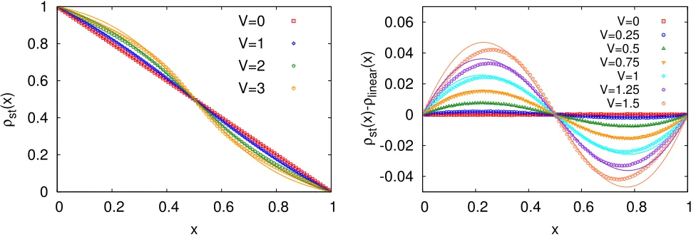
FIG. 1. (Color online) Stationary density profiles forρ0= 1,ρ1 = 0,J= 1 andγ = 1 for increasing values of the interaction strengthV. Solid lines correspond to the analytical density profile derived from equations (13) and (14) while points correspond to the numerical results obtained by simulating the microscopic dynamics given by equation (12) for L = 100. Left panel: Stationary density profiles. Right panel: Difference between the stationary density profiles and the linear one ρlinear(x) = ρ0+ (ρ1−ρ0)x.
the right panel of Fig. 1 deviations from the linear pro-file (V = 0) are displayed; for small values of V (up to V = 0.75) a good agreement is achieved between theory and simulations. Increasing the value of V, we can ob-serve how the numerical results start to deviate from the analytical predictions due to the failure of the mean-field approximation.
IV. STOCHASTIC QUANTUM TRAJECTORIES AND FLUCTUATING HYDRODYNAMICS
We now come back to the original non-interacting model described by equation (1), which is the system we consider in our study. The obtained diffusive charac-ter of the driven quantum chain opens up the possibility of applying MFT [44] for calculating the LD statistics of currents. This would represent a huge simplification as it reduces the non-trivial task of computing the current LD function to a variational problem. Equations (9-11) provide an effective description at the macroscopic level of the exact microscopic master equation, Eqs. (1-4). In order to derive a MFT description we need an equiva-lent macroscopic characterization of the corresponding fluctuating quantum trajectories. In the “input-output” formalism the dynamics of a system operatorXtin terms of both the system and the environment is described in terms of a quantum stochastic differential equation (QSDE) [72] ,
dX=i[H, X]dt+D∗(X)dt (15)
+X
µ
[Vµ†, X]dBµ+dBµ†[X, Vµ]
,
where{Vµ}are the jump operators in the Lindblad mas-ter equation, cf. Eqs. (1-4), and dBµ, dBµ† are
opera-tors on the environment representing a quantum Wiener process and obeying the quantum Ito rules, (dBµ)2 = (dBµ†)2 = dB†
µdBµ = 0 and dBµdBµ† = dt. To under-stand how the quantum trajectories are described at the macroscopic level we consider the simpler case ϕ = 0. In this case, jump operators in the bulk are diagonal in the number operator basis, so that the presence of the environment does not directly affect the evolution of the density. Indeed, the variation in time of a bulk number operator is given by
dnm=− M X
h=1
(jh,mco −jh,mco −h)dt . (16)
The presence of the Wiener process is instead explicit in the stochastic evolution of the quantum current contri-butions; in this case one has
djh,mco ≈
2Jh2(nm−nm+h)−γjh,mco
dt+ +√γ
L X
k=1
[nk, jh,mco ]dBk(t) +dBk†(t)[j co h,m, nm]
,
where we are neglecting those terms that were not con-tributing to the hydrodynamic equation (9) and that can be shown to be irrelevant also in this stochastic regime. The first step is to introduce the time rescaling; it is im-portant to notice that this affects in different ways the two increments: while dt = L2dτ, one has –as for all Wiener processes–dB(t) =LdB(τ). Thus, the rescaled time stochastic equation reads
djh,mco ≈L2
2Jh2(nm−nm+h)−γjh,mco
dτ+ +L√γ
L X
k=1
[nk, jh,mco ]dBk(τ) +dBk†(τ)[j co h,m, nm]
[image:4.612.64.552.55.223.2]
The first term in the above equation is nothing but the deterministic part already present in (7), leading to equa-tion (9). The remaining contribuequa-tion instead, modifies the deterministic equation for the evolution of the macro-scopic density, introducing an extra noisy term (see Ap-pendix B). In particular, rescaling space and considering the largeLlimit, one has that the stochastic macroscopic field ˆρτ obeys the following Langevin equation
∂τρˆτ(x) =−∂xˆjτ(x), (17) where ˆjτ(x) :=−D∂xρˆτ(x) +ξτ(x) indicates the fluctu-ating current field. The coarse-grained macroscopic ef-fects due to the presence of the quantum Wiener process are encoded in the Gaussian noiseξ, determining devia-tions from the average behavior. This zero-mean Gaus-sian noise is characterized by a covariance which, under a local equilibrium assumption for the global quantum state [45], is given by (see Appendix B)
hξτ(x)ξτ0(x0)i=L−1σ( ˆρτ(x))δ(x−x0)δ(τ−τ0), (18) where themobilityσ(ρ) is a function of the density profile
σ(ρ) = 2D ρ(1∓ρ) fermions/bosons. (19) It important to stress the fact that the stochastic macro-scopic fields ˆρτ,ˆjτ represent a coarse-grained hydrody-namic description of the quantum trajectories given by equation (15). The structure of equation (17) remains unchanged for ϕ 6= 0; one only needs to consider the appropriate diffusive parameterD.
Equal densities at the boundaries, %0 = %1 = ρ, corresponds to equilibrium conditions, for which the stationary quantum state is a product thermal one. Thus one can easily compute the compressibility, χ := L−1PL
h,`=1(hnkn`i − hnhihn`i), which can be expressed in terms of the average occupationρas χ(ρ) =ρ(1∓ρ) (for fermions/bosons). This means that theEinstein re-lation [45] connecting the linear response of the density to a perturbation - the mobility - to its spontaneous fluc-tuations in equilibrium - the compressibility - is obeyed, σ(ρ) = 2Dχ(ρ). Notice that we have derivedσ(ρ) start-ing from the quantum trajectories; this extends to generic Hamiltonians the mobility found, by means of pertur-bation theory, for the tight-binding case with dephas-ing [36]. Remarkably, the form of the mobility given by Eq. (19) shows that the fluctuating hydrodynamic behav-ior of these quantum systems is equivalent to the SSEP for fermions and to the SIP for bosons [46–49].
V. CURRENT FLUCTUATIONS, BALLISTIC DYNAMICS AND HYPERUNIFORMITY IN
FERMIONIC CHAINS
The fluctuating hydrodynamics of the quantum chain (17) encodes the evolution of any possible realization
{ρ,ˆ ˆj}of the system. Therefore, not only stationary prop-erties can be derived, but also the dynamical behavior associated with fluctuations and atypical trajectories. In the following, we focus on fermionic chains and study the statistics of the empirical (i.e., time-averaged) total current, ˆq:=T−1R1
0 dx RT
0 dτˆjτ(x), up to a macroscopic time T = t/L2. For long times we expect its probabil-ity to have a LD form, Pt(q) := hδ(q−qˆ)i ≈ e−tφ(q), where φ(q) is the LD rate function. The same infor-mation is encoded in the moment generating function, Zt(s) :=he−s tqi, wheres is thecounting fieldconjugate toq. Zt(s) can be interpreted as a dynamical partition function and allows one to define for eachsa new ensem-ble of trajectories with biased probability, the so-called s-ensemble [54]. Averages in this biased ensemble take the formh·is=Zt(s)−1h(·)e−s tqˆi, withs = 0 being the original non-biased expectation. The dynamical parti-tion funcparti-tion has a LD form, Zt(s)≈etθ(s), where θ(s) is thescaled cumulant generating function(SCGF), and is related to φ(q) via a Legendre transform [50]. The SCGF plays the role of a dynamical free-energy, whose non-analytic behavior accounts for dynamical phase tran-sitions. These correspond to singular changes in the tra-jectories sustaining atypical values of different observ-ables. As shown in [65], the SSEP undergoes a third-order dynamical phase transition for current fluctuations at s = 0. This is reflected in the following limit of the current SCGF obtained in Ref. [65], featuring a discon-tinuity in the third derivative:
˜
θ(s) := lim L→∞
θ(s) L =
σs2
2 +
D√2 24π
σ00σ D2
3/2
|s|3, (20)
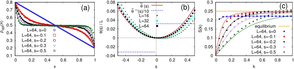
whereσ=σ(ρopt) andσ00=σ00(ρopt) withρoptthe time-independentoptimal profile [73] sustaining the atypical current associated with s. While this dynamical phase transition was already predicted in [65], its physical im-plications at the level of the trajectories is still lacking. In the following, we shall unveil the nature of this tran-sition: while dynamics leading to typical empirical cur-rents is diffusive, the one associated to atypical curcur-rents is ballistic and with hyperuniform spatial structure.
Firstly, we analytically show this change of behavior by means of the FH approach; then we compare our theoret-ical predictions with extensive numertheoret-ical simulations of the rare trajectories of the SSEP, finding good agreement for the largest system size we could reach (L= 64).
Finally, as predicted by (17), we shall show how the FH results correctly describe the hydrodynamics of the quan-tum models introduced in section II through the exact numerical computation of the LD properties of a quan-tum spin chain.
A. Structure factor for rare trajectories
0.1 0.2 0.3 0.4 0.5 0.6 0.7 0.8
0 0.2 0.4 0.6 0.8 1
x
(a)
ρopt
(x)
L=64, s=0 L=64, s=-0.1 L=64, s=-0.2 L=64, s=-0.3 L=64, s=-0.5
-0.04 -0.02 0 0.02 0.04 0.06 0.08
-0.4 -0.2 0 0.2 0.4
(b)
θ
(s) / L
s
θ
~ (s)
θ
~ ’’’(s)/10
L=16 L=32 L=64
0 0.05 0.1 0.15 0.2 0.25 0.3
0 0.2 0.4 0.6 0.8 1 k
(c)
S(k)
equilibrium L=64, s=0 L=64, s=-0.1 L=64, s=-0.2 L=64, s=-0.3 L=64, s=-0.5
FIG. 2. (Color online)Dynamical transition and hyperuniformity in the one-dimensional SSEP with open bound-aries. Here %0 = 0.8,%1=0.2 andD= 1. Lines correspond to analytical predictions while symbols to numerical results. (a) Optimal profiles for four different values ofλ=sLwithL= 64. The numerical results confirm that the profiles tend toρ= 1/2 asλ=sLincreases. (b) SCGF ˜θ(s) given by Eq. (20) (solid red line) together with its third derivative (dashed blue line). (c) Static structure factorS(k,0) for different values of the biass.
structure factor, cf. [74, 75]. In general, this quantity, S(k, t) :=L−1hδ˜n
k(0)δn˜∗k(t)i, is defined in terms of the spatial Fourier transform,δn˜k(t), of the microscopic par-ticle fluctuations, δnm(t) := nm(t)− hnmit. By taking into account the open geometry of the system, this is given by,
δn˜k(t) =√2 L X
h=1
sin(k h)δnh(t)
wherek= πLr, r= 1,2, . . . L−1. By substituting this in the definition of the structure factor one obtains
S(k, t) = 2 L
L X
`,h=1
sin(k `) sin(k h)C`h(t), (21)
withC`h(t) =hδn`(0)δnh(t)isbeing the second cumulant of densities at site hand k averaged in the s-ensemble [54]. While at this microscopic level the computation of density-density correlations is just possible for small sys-tem sizes, one can still derive a closed expression for the structure factor by exploiting the macroscopic approach of fluctuating hydrodynamics. In the large L limit, one can approximate summations with integrals, obtaining the following relation
δn˜k(t) =
√
2L
Z 1
0
dxsin(p x)δρτ(x) =Lδρ˜τ(p), with p = L k, and δρ˜τ(p) being the Fourier sine trans-form of δρτ(x), which encodes the macroscopic den-sity fluctuations around the optimal profile ρopt(x) for a given value of s. Hence we can write S(k, t) in terms of macroscopic quantities, S(k, t) = LS(p, τ) with p = Lk, where S(p, τ) = hδρ˜0(p)δρ˜∗τ(p)is and δρ˜τ(p). These averages over the s-ensemble can be cast in a path-integral representation [76, 77], h·is = e−tθ(s)R
DρDρ¯(·)e−LR
dxdτL[ρ,ρ¯], where ¯ρ is a response field, and the Lagrangian reads
L[ρ,ρ¯] =iρ ∂¯ τρ−D∂x2ρ
−λD∂xρ− σ(ρ)
2 (i∂xρ¯−λ) 2
;
λ=sLis a macroscopic counting field, associated with the average current per site [65, 78]. To evaluateS(p, τ) we need the quadratic expansion of the Lagrangian in terms ofδρandδρ¯,
L2[δρ, δρ¯] =iδρ ∂¯ τδρ−D∂x2δρ
+σ 2(∂xδρ¯)
2 +
−σ
00
4 (i∂xρ¯opt−λ) 2
(δρ)2−iσ0(i∂xρ¯opt−λ)δρ∂xδρ .¯ (22)
Since in general the coefficients in this quadratic expan-sion are space-dependent, the Gaussian integral is non-trivial. However, in the equilibrium case,%0=%1= 1/2, these coefficients become constant, and the integration needed for S(p, τ) becomes straightforward in terms of Fourier modes (see Appendix C). Remarkably, for large
|λ| (i.e. finites), regardless of the density at the bound-aries, the optimal profile tends to maximize σ(ρ), thus adopting the half-filling configurationρ(x) = 1/2, except for vanishingly small regions at the boundaries [65, 75]. This allows for the computation of the structure factor associated with the rare trajectories, which reads (see Appendix C for details),
S(k, t) =σk2exp − t 2
√
4D2k4−2s2σ00σk2 √
4D2k4−2s2σ00σk2 . (23) Notice that the static structure factor associated to equal time density-density correlations is obtained by taking S(k, t= 0).
It follows from (23) that for typical dynamics, s = 0, at equilibrium with%0 =%1= 12, the structure factor is diffusive, S(k, t)∝ exp(−Dk2t). In contrast, and more interestingly, fors 6= 0 and for any value of the density at the boundaries, we get,
S(k, t)∼√ σ|k| −2s2σ00σexp
−|k|t
2 p
−2s2σ00σ
[image:6.612.56.564.52.172.2]
have ballistic dynamical scaling,t≈Lz with dynamical exponent z = 1. (ii) For small k the structure factor vanishes linearly in |k|, i.e. large-scale density fluctua-tions are suppressed and the system becomes spatially
hyperuniform [67]. This shows that for driven fermions the most efficient way to generate dynamics with atypical values of the current is by means of a singular change to a hyperuniform spatial structure, similarly to what occurs in the SSEP with periodic boundaries [74].
B. Simulation and numerical results
The theoretical predictions are based on the assump-tion that the fluctuaassump-tions around the optimal profile are small, so that the Lagrangian can be approximated with its quadratic expansion. To validate this assumption we have performed advanced numerical simulations of the classical stochastic model corresponding to Eq. (17) with σ(ρ) = 2Dρ(1−ρ), namely, the boundary-driven SSEP. These are obtained via the cloning method in continuos time with 1000 clones [79–82]; this method efficiently gen-erates rare trajectories by means of population dynamics techniques similar to those of quantum diffusion Monte Carlo. Figs. 2(a)-(b) display the numerical density pro-files and the associated numerical SCGF, showing good agreement with the MFT predictions. In Fig. 2(c) we observe how the numerical static structure factor follows the theoretical prediction, especially for small values of
|s|. Nevertheless, simulations allow us to explore larger values of s, showing that a hyperuniform spatial struc-ture persists. These computational results confirm the validity of the analytical predictions obtained via the FH approach.
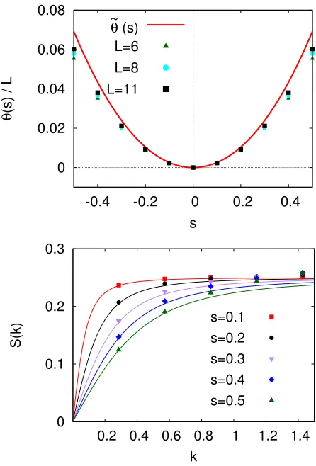
Since we have shown that the quantum trajectories of the models under consideration admit a macroscopic description in terms of Eq. (17), the previous analyt-ical predictions hold as well for the boundary-driven fermionic quantum chains. In order to confirm the va-lidity of our findings, we provide results from exact nu-merical diagonalization of the microscopic quantum tilted generator [56]. We study the case of a fermionic quantum system given by Eq. (1), with M =J1 =γ
in/out 1,L = 1, ϕ = 0, and γ = 2. Following [35, 36], the SCGF for the current in a boundary-driven fermionic chain can be obtained computing the eigenvalues with the largest real part of the tilted generator
Wλ[X] =−i[H, X] +D[X]+ +(eλ−1)aLXa†L+ (e
−λ
−1)a†LXaL.
(25)
We shall consider λ=sL, since we are interested in the total extensive current. Moreover, from the left and right eigenmatrices associated with the largest real eigenvalue of Wλ one can construct the stationary state for each value ofλ[56]. This allows one to compute the density-density correlations necessary to determine the structure factor in the s-ensemble. In Fig. 3 we show the results
0 0.02 0.04 0.06 0.08
-0.4 -0.2 0 0.2 0.4
θ
(s) / L
s θ
~ (s) L=6 L=8 L=11
0 0.1 0.2 0.3
0.2 0.4 0.6 0.8 1 1.2 1.4
S(k)
k
[image:7.612.328.551.51.380.2]s=0.1 s=0.2 s=0.3 s=0.4 s=0.5
FIG. 3. (Color online) Top panel: SCGF for a fermionic quantum system given by the largest eigenvalue of Eq. (25) for different system sizes (symbols), together with the SCGF, ˜
θ(s), predicted by fluctuating hydrodynamics Eq. (20) (solid red line). Bottom panel: Structure factor for L = 11 for different values ofs, along with the fluctuating hydrodynamic prediction (solid lines).
for the SCGF forL = 6,8,11, together with the static structure factor for L = 11. This is the largest size we could reached with exact numerical diagonalization of this quantum problem. In the top panel, we can ob-serve a good convergence towards the predicted SCGF with the system size. Remarkably, in the bottom panel the numerical results of the structure factor show a good agreement with the FH predictions already forL = 11. These results confirm the equivalence between the fluc-tuating hydrodynamics of fermionic chains and SSEPs, predicted by Eq. (17).
VI. CONCLUSIONS
dephasing where interactions give rise to a density de-pendent diffusion coefficient. Furthermore, starting from an unravelling of the open quantum dynamics in terms of stochastic quantum trajectories we have derived, for the non-interacting case, an effective fluctuating hydrody-namic that describes fluctuations in microscopic trajecto-ries at a coarse-grained level. Interestingly, this effective description is equivalent to the fluctuating hydrodynam-ics of classical simple exclusion/inclusion processes for fermionic/bosonic systems. Exploiting this analogy, we have shown that fermionic chains undergo a dynamical phase transition at the level of fluctuations, from a phase corresponding to typical diffusive dynamics when trajec-tories are conditioned on having typical values of (time-integrated) currents, to a phase with ballistic dynamics and hyperuniform spatial structure when trajectories are conditioned on atypical values of currents. Our theoret-ical predictions are confirmed both by extensive numer-ical simulations of rare trajectories in the open classnumer-ical SSEPs - in particular corroborating the dynamical struc-ture factors obtained from the FH approach - and via ex-act numerical diagonalization of the quantum tilted gen-erator - indicating the validity of the effective FH descrip-tion of the open quantum chains. It would be interesting to experimentally probe our predicted phase transitions by monitoring current fluctuations in boundary-driven cold atomic lattice systems, for example via a variant of the experiment reported in Ref. [83].
ACKNOWLEDGMENTS
This work was supported by EPSRC Grant No. EP/M014266/1, H2020 FET Proactive project RySQ (Grant No. 640378), and ERC Grant Agreement No. 335266 (ESCQUMA). We are also grateful for access to the University of Nottingham High Performance Com-puting Facility.
Appendix A: Effective macroscopic description
We present the derivation of the effective diffusive equation, Eq. (9), governing the dynamics of the coarse-grained particle density profile of the quantum chain. First of all, we provide a relation that will be extensively used throughout the derivation: it can be checked that
lim L→∞L
2Z t
0
due−L2γ(t−u)fL(u) = 1
γf∞(t), (A1) whenever {fL(u)}L is a sequence of bounded functions
∀u > 0, converging in L; namely, L2 times the expo-nential converges weakly (under integration) to a Dirac deltaδ(t−u).
Given the quantum master equation∂tXt=i[H, Xt] +
D∗[Xt], we are interested in deriving an effective dynam-ics for the average density of particles in the rescaled
coordinates,τ = t/L2, mL → x∈ [0,1]. The time-scale t/L2can be simply obtained by multiplying the action of the generator by a factorL2,
∂τXτ=L2(i[H, Xτ] +D∗[Xτ]).
Regarding the spatial dimension, coarse-graining consists in mapping theL-site chain onto a line Λ = [0,1], in such a way that them-th site of the chain corresponds to the point mL in Λ. In order to account for this geometric mapping, one has to notice that for largeL, the spacing between sites in Λ, equal to 1
L, becomes infinitesimal. We now introduce a continuous description; namely, we inter-preta†mas the creator of a particle in the one-dimensional box centred in mL of width L1. Mathematically, by means of the continuous fields
αx, α†x x∈Λ, one has
a†m=
√
L
Z
Um dx α†x
where Um is the domain of the box across the point m
L ∈ Λ; the multiplying factor
√
L is needed to guar-antee the commutation (anti-commutation) relations of the discrete bosonic (fermionic) operators, starting from the continuous ones for αx, α†x. Moreover, the integral can be approximated for largeL by
a†m∼ √1
Lα †
m
L . (A2) With this at hand, we have all the ingredients to per-form the hydrodynamic limit. We shall first consider the simplest case of a tight-binding Hamiltonian and then extend the result to more general situations.
1. Nearest-neighbour coherent hoppingM = 1
In this section we focus on the tight-binding Hamil-tonian H = JPL−1
k=1
a†k+1ak+a†kak+1
; its action on quadratic operators reads
iH, a†man
=iJ∆2L a†m
an−a†m∆ 2 L(an)
, (A3) with
∆2L(Xm) =Xm+1−2Xm+Xm−1.
For a generic bulk sitem, the rescaled time-derivative of the expectation of the number operatornm=a†mamcan be cast in the following form
∂τhnmiτ =−L2 hjcom−j co
m−1iτ+hjmdis−j dis m−1iτ
; (A4) the operatorjcom has the meaning of a coherent current through the sitesm,m+ 1 and is defined as
jmco:=−iJa†m+1am−a†mam+1
while
jmdis:=ϕ(nm−nm+1).
To close the equation for the number operators, one needs to work on the currentjco
m. In particular, given the dis-sipatorD∗and by using (A3), itsτ time-derivative reads
∂τjmco=L 2
2J2(nm−nm+1) +J2Qm−γj˜ mco
, (A6) with
Qm=a†m+2am+a†mam+2−a†m+1am−1−a†m−1am+1, (A7) and ˜γ=γ+ 2ϕ >0. The termQmwill be shown not to contribute in the hydrodynamic limit, but still its deriva-tive needs to be considered:
∂τQm=L2(−γQ˜ m+i[H, Qm]) ; (A8) we will study later the action of the Hamiltonian on this operator. Now, by formally integrating (A6) and (A8) and by substituting the result for Qm into the time-evolution of the coherent current, we get
hjcomiτ ∼ −2J2L2 Z τ
0
due−L2γ˜(τ−u)∆Lhnmiu+
+L4
Z τ
0
du
Z u
0
dve−L2˜γ(τ−v)ih[H, Qm]iv, (A9)
with ∆Lnm=nm+1−nm and where we have neglected exponentially decaying terms inL. To proceed, we sub-stitute the above result, forjco
m, jmco−1, in equation (A4). By doing this and rearranging terms we find
∂τhnmiτ= 2J2L4 Z τ
0
due−L2γ˜(τ−u)∆2Lhnmiu+
+ϕL2∆2Lhnmiτ−iJ2L6 Z τ
0 Z u
0
dudve−L2˜γ(τ−v)hPmiv, (A10)
with Pm = [H, Qm−Qm−1]. Considering relation (A2) and noticing that Pm is quadratic in bosonic/fermionic operators, we introduce the operator ˜Pm
L, which is the quadratic operator resulting fromPm, just by replacing the discrete field with the continuous ones. In this way one is able to write the following differential equation for the expectation ofηx=α†xαx
∂τhηm
Liτ = 2J
2
L4
Z τ
0
due−L2γ˜(τ−u)∆2LhηmLiu+ +ϕL2∆2Lhηm
Liτ−iJ
2L6Z τ
0 Z u
0
dudve−L2γ˜(τ−v)hP˜m Liv. (A11)
The term L2∆2
LhηmLiτ represents a finite difference sec-ond derivative of the density, which in the largeL limit with m
L →xbecomes lim L→∞ϕ L
2∆2
LhηmLiτ=ϕ ∂
2
xhηxiτ. (A12)
Similarly, taking also into account (A1), one has
lim L→∞2J
2L4Z τ
0
due−L2γ˜(τ−u)∆2Lhηm Liu=
2J2 ˜ γ ∂
2 xhηxiτ. It remains to show that the last term of the r.h.s of equation (A11) does not contribute in the large L limit. Firstly, one can check that the following quantity is bounded:
lim L→∞J
2L4 Z τ
0
du
Z u
0
dve−L2˜γ(τ−v)=C <∞.
As a consequence the modulus of the last term in (A11)
I= lim L→∞
J2L6
Z τ
0 Z u
0
dudve−L2γ˜(τ−v)hP˜m Liv
(A13)
can be bounded by
I≤C lim L→∞max∀t>0
n
L2 h
˜ Pm
Lit
o
. (A14)
To understand the contribution of the operator ˜Pm L, one needs to go back to the operatorQm. The latter is made of the product of operators spaced by two lattice sites. For example, by using equation (A3), one has
i[H, a†m+2am] =iJ∆2L(a †
m+2)am−a†m+2∆ 2 L(am)
; (A15) then, by multiplying by L2 and considering the spatial scaling one has
lim L→∞L
2h∆2 L(α
† m+2
L )αm
L−α †
m+2
L
∆2L(αm L)it= = h∂x2α†xαxit− hα†x∂
2 xαxit
. (A16)
Due to the spatial coarse-graining, all terms of [H, Qm] give the same hydrodynamic contribution equal to (A16). Since Qm is made of two terms with positive sign and another two with negative one, the net result for the hy-drodynamic limit ofh[H, Qm]iτ is zero. This implies that in the large L limit L2hP˜m
Lit → 0. Thus, by defining ρτ(x) =hηxiτ, we have shown that (A11) reads
∂τρτ(x) =
ϕ+ 2J 2
γ+ 2ϕ
∂x2ρτ(x), (A17)
which corresponds to Eq. (9) forM = 1.
Such a differential equation needs to be provided with two boundary conditions; these are given by the extremal sites of the chain. For the expectation value of the num-ber operator of the first sitea†1a1, one has
∂τha†1a1iτ =L2 h
γin1 −(γout1 ±γin1 )ha
†
1a1iτ+
+iJha†2a1−a†1a2iτ+ϕha†2a2−a†1a1iτ i
where the plus is for fermionic systems while the mi-nus for bosonic ones. In the latter case, γout
1 −γin1 >0 is needed for the convergence of the expectations. For-mally integrating the above equation we get, neglecting exponentially decaying terms,
ha†1a1iτ− γin
1
γout 1 ±γ1in
≈L2
Z τ
0
due−L2(γout1 ±γin1 )(τ−u)×
×iJha†2a1−a†1a2iu+ϕha†2a2−a†1a1iu
. (A19)
The right-hand side of the above relation, using (A1), going to the continuous description, and using that
lim L→∞hα
†
2
L α1
L−α †
1
L α2
Liu= 0,Llim→∞hα †
2
L α2
L−α †
1
L α1
Liu= 0, can be shown to go to zero in the large L limit. Thus, one finds that the left boundary density is given by
%0= lim L→∞ha
†
1a1iτ= γ1in
γout 1 ±γin1
. (A20)
Similarly, at the right boundary one has
%1= lim L→∞ha
† LaLiτ=
γLin γout
L ±γ in L
, (A21)
providedγout L ±γ
in L >0.
2. Short-range coherent particle hopping (M finite)
The starting point in this case is the time-rescaled dif-ferential equation (6). As before, one needs to work on the generic quantum current contributionjh,mco ; its time-derivative can be casted in the following form
∂τjcoh,m=L 2h2J2
h(nm−nm+h) +Jh2Q h m+ +Jh
X
`6=h
J`Qh,`m −˜γj co h,m
i
. (A22)
The termQh
mis a generalization ofQmof equation (A7), and reads
Qhm=a†m+2ham−a†m+ham−h−a†m−ham+h+a†mam+2h, while, by defining ∆2L,`(Xm) = Xm+`−2Xm+Xm−`, Qh,`
m can be written as
Qh,`m = ∆ 2 L,`(a
†
m+h)am−a†m+h∆ 2
L,`(am)+
−∆2L,`(a†m)am+h+a†m∆ 2
L,`(am+h).
(A23)
One can show that, in the hydrodynamic limit, neither Qh
mnorQh,`m , contribute to the differential equation. Re-gardingQhm, this can be shown by performing analogous manipulations to the ones involved in the discussion of the term Qm in the previous case. For Qh,`m, we show
below that the contribution is vanishing in the limit of largeL.
Let us focus on the first summand of the right-hand side of the above equation, written in terms of the con-tinuous creation and annihilation operators α†
x, αx (see (A2)) and multiplied by the time-rescaling factor L2. One has, withx=m/L
L2∆2L,`α† x+h
L
αx=`2 α†
x+h+L` −2α
† x+h
L +α†
x+hL−` `
L
2 αx.
In the largeLlimit, considering thath/L→0 and`/L→
0, this term becomes
lim L→∞L
2∆2 L,`
α†x+h L
αx=`2∂x2α † xαx.
Moreover, also the third term on the right-hand side of equation (A23) converges to the same second order derivative obtained above, and, since it appears inQh,`m with a minus sign, it cancels the contribution given by the first term Qh,`
m. The same happens for the remain-ing two terms. Therefore, formally integratremain-ingjco
h,m and substituting the result in the equation for the number operator (6), the hydrodynamic contribution from Qh,` m vanishes. We thus have that the differential equation for the evolution of the densityhηxi=hα†xαxi, which reads
∂τhηm Liτ =L
2ϕ∆2
L(hηmLi)+ + 2
M X
h=1
Jh2L4
Z τ
0
due−L2γ˜(τ−u)∆2L,hhηm Liu.
(A24)
Taking into account relation (A1) and given that, with x= mL,
lim L→∞L
2∆2
L,hhnmiτ=h2∂x2hηxiτ
one obtains in the hydrodynamic limit, with ρτ(x) =
hηxiτ,
∂τρτ(x) = "
ϕ+ 2 γ+ 2ϕ
M X
h=1
Jh2h 2
#
∂x2ρτ(x),
which corresponds to Eq. (9) for finiteM.
Appendix B: fluctuating hydrodynamics
We start from the time-rescaled equations
dnm=−L2 M X
h=1
(jcoh,m−jh,mco −h)dτ; (B1)
and
djh,mco ≈L2
2Jh2(nm−nm+h)−γjh,mco
dτ+ +L√γ
L X
k=1
[nk, jh,mco ]dBk(t) +dBk†(t)[j co h,m, nm]
where, in the latter, we have neglected the termQhmand Qh,`
m of (A22) that, as in the deterministic case of the previous section, can be shown not to contribute to the effective equation. By manipulating the noise term, the above equation can be rewritten as
djh,mco ∼L2
2Jh2(nm−nm+h)−γjh,mco
dτ +L√γJhXh,mdNh,m(τ), withXh,m=a†m+ham+a†mam+h and
dNh,m(τ) =−i
dBm+h(τ)−dB†m+h(τ)
+
+i dBm(τ)−dBm† (τ)
. Integrating the above differential equation forjco
h,m, and substituting it in the equation (B1) one finds, using re-lation (A1),
dnm= 2 γ
M X
h=1
Jh2L2∆2L,h(nm)dτ+
−
M X
h=1
Jh
√
γ(Xh,mdNh,m(τ)−Xh,m−hdNh,m−h(τ)), (B2)
where we have used (A1) and neglected the exponentially decaying term inL. Moving to the continuous coordinate given by (A2), again with ηx =α†xαx, x= mL, one gets, with ∆L,h(Ox) =Ox−Ox−h
L,
∂τηx= 2 γ
M X
h=1
Jh2L2∆2L,h(ηx)+
−L M X
h=1 ∆L,h
J
h
√
Lγ ˜ Xh,x
dνh,x(τ) dτ
,
(B3)
with ˜Xh,x being the analogous operator of Xh,m but written in terms of the continuous fields αx, α†x; dνh,x is also the analogous operator of dNh,m(τ), but writ-ten in term of the coarse-grained environment’s opera-torsdβx(τ), dβx†(τ). In particular, the analogous relation to (A2) holds
dB†m(τ)∼ 1
√
Ldβ † x(τ), which is responsible, for the extra factor √1
L in the round brackets of equation (B3). We see in (B3) the same de-terministic diffusion term of (A24) (forϕ= 0) minus the first derivative of a noise term, that we denote byξτ(x),
ξτ(x) = M X
h=1
Jh
√
Lγh ˜ Xh,x
dνh,x(τ) dτ .
The factor h multiplying each term of the sum is due to the fact that ∆L,h converges, in the hydrodynamic
limit, to h times the first derivative with respect to x. Thus, the evolution equation for the fluctuating density ˆ
ρτ(x) =hηxiτ is given by
∂τρˆτ(x) =D∂x2ρˆτ(x)−∂xξτ(x), where the noise termξτ(x) has a covariance
hξτ(x)ξτ0(y)i=
σ( ˆρτ(x))
L δ(x−y)δ(τ−τ 0), σ(ρ) = 2Dρ(1±ρ), where the plus stands for bosons and the minus for fermions. This covariance can be derived by directly computing
hξτ(x)ξτ0(y)i= M X
h,`=1
JhJ`h` Lγ ×
×
˜ Xh,xX˜`,y
dνh,x(τ) dτ
dν`,y(τ0) dτ0
.
To understand the contribution of the operator ˜Xh,xX˜`,y withx= mL, y= nL, we look at the discrete original one Xh,mX`,n=
a†m+ham+a†mam+h a†n+`an+a†nan+`
;
expanding the product one gets
Xh,mX`,n=a†m+hama†n+`an+a†mam+ha†n+`an+ +a†m+hama†nan+`+a†mam+ha†nan+`. Due to the presence of dephasing, damping quantum co-herences on fastest time-scales than those ofτ, we assume a local “thermal” equilibrium state for the infinitesimal domain across the bondsx= mL, y =Ln [45] . This local equilibrium assumption implies that we have to consider only those terms inXh,mX`,ngiving a non-zero expecta-tion over a free thermal equilibrium state. This happens only whenm=nandh=`, where one has
hXh,m2 i ∼ hnm(1±nm+h) +nm+h(1±nm)i Hence, the contribution of the coarsed-grained operator
˜
Xh,x2 reads
hX˜2
h,xi= 2 ˆρτ(x) (1±ρˆτ(x)),
where the plus stands for bosons and the minus for fermions, and with ˆρτ(x) being the fluctuating parti-cle density. Taking into account also the contribution of Ddνh,x(τ)
dτ
dνh,y(τ0) dτ0
E
, one has that the non-vanishing
terms areDX˜h,xX˜h,y
dνh,x(τ) dτ
dνh,y(τ0) dτ0
E
= 4δ(x−y)δ(τ−
τ0) ˆρ
τ(x) (1±ρˆτ(x)) and thus, the full covariance of the noiseξτ(x) is given by
hξτ(x)ξτ0(y)i= 4 M X
h=1
J2 hh
2
Lγ ρˆτ(x) (1±ρˆτ(x))×
This means that, starting from the quantum stochas-tic master equation describing the quantum trajectories of the microscopic evolution, the equation governing the fluctuating hydrodynamics in the coarse-grained macro-scopic description reads
∂τρˆτ(x) =−∂xˆjτ(x), ˆjτ(x) =−D∂xρˆτ(x) +ξτ(x),
withD= 2PM h=1
J2
hh2
γ , andξτ(x) a noise with properties already discussed. The same result holds if one considers ϕ6= 0, i.e. withD=ϕ+2
PM
h=1Jh2h2 γ+2ϕ .
Appendix C: Derivation of the structure factor
In this section we provide details on the computation of the dynamical structure factor. As pointed out above, in the large |λ|regime one has that the stationary opti-mal profileρopt(x) tends to the valueρopt→1/2 almost everywhere, except for vanishingly small regions at the boundaries. As a consequence σ(ρopt) → σ = 1/2, so thatσ0 →0. Moreover ¯ρoptis such that∂xρ¯opt→0 [65]. Thus, one can approximateL2 with
L2∼Lˆ2=iδρ ∂¯ τδρ−D∂2xδρ
+σ 2(∂xδρ¯)
2 −σ
00
4 λ 2(δρ)2,
(C1) with L2 = ˆL2 only in the L → ∞ limit, for s 6= 0. Notice that ˆL2 is the exact second order expansion of the LagrangianLin the equilibrium case%0=%1= 1/2. Therefore, for largeL, the expectation in the s-ensemble is well approximated by
hOis∼ R
DρDρO¯ [ρ]e−LRR
dxdτLˆ2[δρ,δρ¯]
R
DρDρ¯e−LRR
dxdτLˆ2[δρ,δρ¯]
, (C2)
which can be computed as we show in the following. Through the space-time Fourier expansion,
δρτ(x) =
√
2 T
X
ω X
p>1
sin(p x)e−iωτδρ˜p,ω
withω= 2Tπu, u∈Z, and, the equivalent one forδρ¯τ(x), one can diagonalise ˆL2, obtaining
Z Z
dxdτLˆ2= 1 T
X
p>1,ω≥0
δ~ρ˜p,ω† ·Kp,ω·δ~ρ˜p,ω,
whereδ~ρ˜p,ω = (δρ˜p,ω, δρ˜¯p,ω)tr (with atr denoting vector transposition anda†= (a∗)tr), and
Kp,ω =
−σ00λ2
2 ω+iDp
2
−ω+iDp2 σp2
.
At this point, the computation of S(p, τ) is reduced to evaluations of Gaussian path integrals. In terms of the Fourier fieldsδρ˜p,ω,
δρ˜τ(p) = 1 T
X
ω
e−iωτδρ˜p,ω, (C3) one can write
S(p, τ) = 1 T2
X
ω,ω0
eiωτhδρ˜p,ω0δρ˜∗p,ωis.
Then, evaluating the aboves-ensemble expectation with (C2), one gets
hδρ˜p,ωδρ˜∗p,ω0is∼δω,ω0 T L
σp2
ω2+D2p4−λ2σ00σp2
2
.
ThusS(p, τ) reads
S(p, τ)∼ 1
LT
X
ω
eiωτ σp
2
ω2+D2p4−λ2σ00p2
2
.
By replacing the summation overω with an integration in the long-time limit,S(p) reads
S(p, τ) = 1 2πL
Z ∞
−∞
dωeiωτ σp 2
ω2+D2p4−λ2σ00p2
2
.
Therefore, one finds
S(p, τ) =1 L
σp2 p
4D2p4−2λ2σ00σp2× ×exp−τ
2 p
4D2p4−2λ2σ00σp2.
(C4)
Recalling thatλ=sL,p=Lk, and that in the large L limit approximations (C1)-(C2) become exact, one has
S(k, t) =σk2exp − t 2
√
4D2k4−2s2σ00σk2 √
4D2k4−2s2σ00σk2 . (C5)
[1] A. Polkovnikov, K. Sengupta, A. Silva, and M. Vengalat-tore, Rev. Mod. Phys.83, 863 (2011).
[3] L. D’Alessio, Y. Kafri, A. Polkovnikov, and M. Rigol, Adv. Phys.65, 239 (2016).
[4] F. H. L. Essler and M. Fagotti, J. Stat. Mech. , P064002 (2016).
[5] R. Vasseur and J. E. Moore, J. Stat. Mech. , P064010 (2016).
[6] R. Nandkishore and D. A. Huse, Annu. Rev. Condens. Matter Phys.6, 15 (2015).
[7] R. Moessner and S. Sondhi, Nature Phys.14, 424 (2017). [8] T. Langen, S. Erne, R. Geiger, B. Rauer, T. Schweigler, M. Kuhnert, W. Rohringer, I. E. Mazets, T. Gasenzer, and J. Schmiedmayer, Science 348, 207 (2015).
[9] M. Schreiber, S. S. Hodgman, P. Bordia, H. P. L¨uschen, M. H. Fischer, R. Vosk, E. Altman, U. Schneider, and I. Bloch, Science349, 842 (2015).
[10] J. Choi, S. Hild, J. Zeiher, P. Schauß, A. Rubio-Abadal, T. Yefsah, V. Khemani, D. A. Huse, I. Bloch, and C. Gross, Science352, 1547 (2016).
[11] J. Zhang, P. Hess, A. Kyprianidis, P. Becker, A. Lee, J. Smith, G. Pagano, I.-D. Potirniche, A. Potter, A. Vish-wanath,et al., Nature543, 217 (2017).
[12] P. Bordia, H. L¨uschen, U. Schneider, M. Knap, and I. Bloch, Nature Phys.13, 460 (2017).
[13] S. Choi, J. Choi, R. Landig, G. Kucsko, H. Zhou, J. Isoya, F. Jelezko, S. Onoda, H. Sumiya, V. Khemani, et al., Nature543, 221 (2017).
[14] S. Jezouin, F. D. Parmentier, A. Anthore, U. Gennser, A. Cavanna, Y. Jin, and F. Pierre, Science 342, 601 (2013).
[15] R. Nandkishore, S. Gopalakrishnan, and D. A. Huse, Phys. Rev. B90, 064203 (2014).
[16] E. Levi, M. Heyl, I. Lesanovsky, and J. P. Garrahan, Phys. Rev. Lett.116, 237203 (2016).
[17] M. H. Fischer, M. Maksymenko, and E. Altman, Phys. Rev. Lett. 116, 160401 (2016).
[18] M. V. Medvedyeva, T. Prosen, and M. Znidaric, Phys. Rev. B93, 094205 (2016).
[19] H. P. L¨uschen, P. Bordia, S. S. Hodgman, M. Schreiber, S. Sarkar, A. J. Daley, M. H. Fischer, E. Altman, I. Bloch, and U. Schneider, Phys. Rev. X 7, 011034 (2017). [20] C. Monthus, J. Stat. Mech. , P043302 (2017).
[21] D. Bernard and B. Doyon, Annales Henri Poincar´e 16, 113 (2015).
[22] D. Bernard and B. Doyon, J. Stat. Mech. , P033104 (2016).
[23] D. Bernard and B. Doyon, J. Stat. Mech. , P064005 (2016).
[24] O. A. Castro-Alvaredo, B. Doyon, and T. Yoshimura, Phys. Rev. X6, 041065 (2016).
[25] B. Bertini, M. Collura, J. De Nardis, and M. Fagotti, Phys. Rev. Lett.117, 207201 (2016).
[26] M. Ljubotina, M. Znidaric, and T. Prosen, Nature Comm.8, 16117 EP (2017).
[27] T. Prosen, Phys. Rev. Lett.107, 137201 (2011). [28] M. Znidaric, B. Zunkovic, and T. Prosen, Phys. Rev. E
84, 051115 (2011).
[29] M. Znidaric, J. Phys. A43, 415004 (2010). [30] M. Znidaric, J. Stat. Mech. , PL05002 (2010). [31] M. Znidaric, Phys. Rev. E83, 011108 (2011). [32] V. Eisler, J. Stat. Mech. , P06007 (2011).
[33] K. Temme, M. M. Wolf, and F. Verstraete, New J. Phys.
14, 075004 (2012).
[34] B. Buca and T. Prosen, Phys. Rev. Lett. 112, 067201 (2014).
[35] M. Znidaric, Phys. Rev. Lett.112, 040602 (2014). [36] M. Znidaric, Phys. Rev. E89, 042140 (2014).
[37] E. Ilievski and T. Prosen, Nuclear Physics B 882, 485 (2014).
[38] T. Prosen, J. Phys. A48, 373001 (2015). [39] E. Ilievski, arXiv:1612.04352 (2016).
[40] D. Karevski, V. Popkov, and G. Sch¨utz, arXiv:1612.03601 (2016).
[41] C. Monthus, J. Stat. Mech. , P043303 (2017).
[42] V. Popkov and G. M. Sch¨utz, Phys. Rev. E 95, 042128 (2017).
[43] B. Derrida, J. Stat. Mech. , P07023 (2007).
[44] L. Bertini, A. De Sole, D. Gabrielli, G. Jona-Lasinio, and C. Landim, Rev. Mod. Phys.87, 593 (2015).
[45] H. Spohn,Large Scale Dynamics of Interacting Particles
(Spinger Verlag, 1991).
[46] C. Giardina, J. Kurchan, and F. Redig, J. Mat. Phys.
48, 033301 (2007).
[47] C. Giardina, F. Redig, and K. Vafayi, J. Stat. Phys.141, 242 (2010).
[48] G. Carinci, C. Giardin`a, C. Giberti, and F. Redig, J. Stat. Phys.152, 657 (2013).
[49] Y. Baek, Y. Kafri, and V. Lecomte, J. Stat. Mech. , P053203 (2016).
[50] H. Touchette, Phys. Rep.478, 1 (2009).
[51] P. I. Hurtado, C. P. Espigares, J. J. del Pozo, and P. L. Garrido, J. Stat. Phys.154, 214 (2014).
[52] A. Lazarescu, J. Phys. A48, 503001 (2015).
[53] T. Bodineau and B. Derrida, Phys. Rev. E72, 066110 (2005).
[54] J. P. Garrahan, R. L. Jack, V. Lecomte, E. Pitard, K. van Duijvendijk, and F. van Wijland, Phys. Rev. Lett.98, 195702 (2007).
[55] V. Lecomte, C. Appert-Rolland, and F. van Wijland, J. Stat. Phys.127, 51 (2007).
[56] J. P. Garrahan and I. Lesanovsky, Phys. Rev. Lett.104, 160601 (2010).
[57] P. I. Hurtado and P. L. Garrido, Phys. Rev. Lett.107, 180601 (2011).
[58] A. Gambassi and A. Silva, Phys. Rev. Lett.109, 250602 (2012).
[59] C. P. Espigares, P. L. Garrido, and P. I. Hurtado, Phys. Rev. E87, 032115 (2013).
[60] D. Manzano and P. I. Hurtado, Phys. Rev. B90, 125138 (2014).
[61] P. Tsobgni Nyawo and H. Touchette, Phys. Rev. E94, 032101 (2016).
[62] N. Tiz´on-Escamilla, C. P´erez-Espigares, P. L. Garrido, and P. I. Hurtado, Phys. Rev. Lett.119, 090602 (2017). [63] Y. Baek, Y. Kafri, and V. Lecomte, Phys. Rev. Lett.
118, 030604 (2017).
[64] A. Lazarescu, J. Phys. A50, 254004 (2017).
[65] A. Imparato, V. Lecomte, and F. van Wijland, Phys. Rev. E80, 011131 (2009).
[66] V. Lecomte, A. Imparato, and F. v. Wijland, Prog. Th. Phys. Supp.184, 276 (2010).
[67] S. Torquato, Phys. Rev. E94, 022122 (2016). [68] G. Lindblad, Comm. Math. Phys48, 119 (1976). [69] V. Gorini, A. Kossakowski, and E. C. G. Sudarshan, J.
Mat. Phys.17, 821 (1976).
[70] M. ˇZnidariˇc, Phys. Rev. E92, 042143 (2015).
[72] C. Gardiner and P. Zoller, Quantum noise (Springer, 2004).
[73] O. Shpielberg and E. Akkermans, Phys. Rev. Lett.116, 240603 (2016).
[74] R. L. Jack, I. R. Thompson, and P. Sollich, Phys. Rev. Lett.114, 060601 (2015).
[75] D. Karevski and G. M. Sch¨utz, Phys. Rev. Lett. 118, 030601 (2017).
[76] H. Janssen,From Phase Transitions to Chaos(World Sci-entific, 1992).
[77] J. Tailleur, J. Kurchan, and V. Lecomte, J. Phys. A41, 505001 (2008).
[78] C. Appert-Rolland, B. Derrida, V. Lecomte, and F. van Wijland, Phys. Rev. E78, 021122 (2008).
[79] C. Giardina, J. Kurchan, and L. Peliti, Phys. Rev. Lett.
96, 120603 (2006).
[80] V. Lecomte and J. Tailleur, J. Stat. Mech. , P03004 (2007).
[81] J. Tailleur, V. Lecomte, J. Marro, P. L. Garrido, and P. I. Hurtado, inAIP Conference Proceedings, Vol. 1091 (AIP, 2009) pp. 212–219.
[82] C. Giardina, J. Kurchan, V. Lecomte, and J. Tailleur, J. Stat. Phys.145, 787 (2011).