BayesPiles : visualisation support for Bayesian network structure learning

BayesPiles: Visualisation Support for Bayesian Network Structure

Learning

ATHANASIOS VOGOGIAS,

JESSIE KENNEDY,

DANIEL ARCHAMBAULT,

BENJAMIN BACH,

V ANNE SMITH,

HANNAH CURRANT,

We address the problem of exploring, combining and comparing large collections of scored, directed networks for understanding inferred Bayesian networks used in biology. In this field, heuristic algorithms explore the space of possible network solutions, sampling this space based on algorithm parameters and a network score that encodes the statistical fit to the data. The goal of the analyst is to guide the heuristic search and decide how to determine a final consensus network structure, usually by selecting the top-scoring network or constructing the consensus network from a collection of high-scoring networks. BayesPiles, our visualisation tool, helps with understanding the structure of the solution space and supporting the construction of a final consensus network that is representative of the underlying dataset. BayesPiles builds upon and extends MultiPiles to meet our domain requirements. We developed BayesPiles in conjunction with computational biologists who have used this tool on datasets used in their research. The biologists found our solution provides them with new insights and helps them achieve results that are representative of the underlying data.

CCS Concepts: •Human-centered computing→Information visualization;Graphical user interfaces;

•Computing methodologies→Bayesian network models;•Applied computing→Biological networks;

Additional Key Words and Phrases: Visualisation, Graphs, Bioinformatics

ACM Reference format:

Athanasios Vogogias, Jessie Kennedy, Daniel Archambault, Benjamin Bach, V Anne Smith, and Hannah Currant. 2017. BayesPiles: Visualisation Support for Bayesian Network Structure Learning.ACM Trans. Intell. Syst. Technol.0, 0, Article 0 ( 2017),23pages.

DOI: 0000001.0000001

Authors’ addresses: A. Vogogias, School of Computing, Edinburgh Napier University, 10 Colinton Road, Edinburgh, EH10 5DT, UK; J. Kennedy, School of Computing, Edinburgh Napier University, 10 Colinton Road, Edinburgh, EH10 5DT, UK; D. Archambault, School of Computer Science, Swansea University, Swansea, UK; B. Bach, The University of Edinburgh, School of Informatics, Informatics Forum, 10 Crichton St, Edinburgh, UK; V.A. Smith, School of Biology, University of St Andrews, Sir Harold Mitchell Building, Greenside Place, St Andrews, UK; H. Currant, The European Bioinformatics Institute (EMBL-EBI), Wellcome Genome Campus, CB10 1SD, UK..

Permission to make digital or hard copies of all or part of this work for personal or classroom use is granted without fee provided that copies are not made or distributed for profit or commercial advantage and that copies bear this notice and the full citation on the first page. Copyrights for components of this work owned by others than the author(s) must be honored. Abstracting with credit is permitted. To copy otherwise, or republish, to post on servers or to redistribute to lists, requires prior specific permission and/or a fee. Request permissions from [email protected].

4. Construct consensus network:

Inform

parameters

BayesPiles

Heuristic Search

1. Find network

structures 2. Score networkstructures Network Score struct 01 - 3700.3 struct 02 - 3699.9 struct 03 - 3701.2 struct 04 - 3697.1 ... ...

Import results

3. Determine shape of solution space:

- Select high-scoring networks - Filter out edges

Flat

Single optimum

Multiple optima

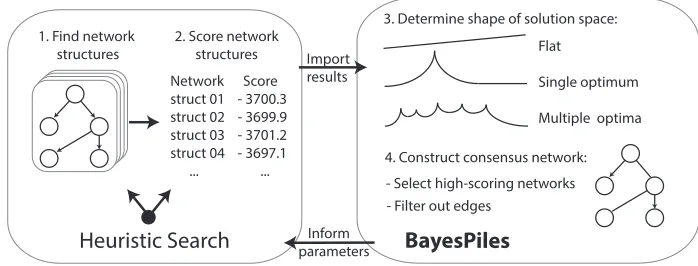
Fig. 1. An overview of the workflow. BayesPiles visualises the results of heuristic search algorithms, informs their parameter settings and enables the construction of a consensus network structure.

1 INTRODUCTION

Network models are used to describe complex interactions and provide an abstract view on how systems work as a whole [29]. For instance, in biological network models, nodes can encode biological components such as genes, RNA, proteins and metabolites, and edges represent direct or combinatorial relationships, such as activation and inhibition. However, collecting data about such relationships is highly complex and may result from multiple measurements. As a consequence, measurements might be noisy, sparse, and can contain missing values [17,32]. These factors add to the uncertainty about the state of the complex natural system (the network) and which hence becomes inherently stochastic.

To model such complex and uncertain biological systems, probabilistic graphical models gained popularity over deterministic methods, due to their ability to handle uncertainty and their ease of interpretation. Probabilistic models provide a clear and compact representation of the data and encapsulate details such as the parameterisation of the probability distribution. Their simplicity highlights their qualitative nature and enables modellers to combine mathematical and computa-tional methods with their own tacit knowledge to take decisions about the final structure of the model [34,39]. Eventually, these models are key in supporting modellers in gaining insight into biological systems and to develop better and more useful graphical models from experimental data.

One type of graphical model is Bayesian networks [34]. Bayesian networks (BNs) are directed acyclic graphs (DAGs) with nodes representing random variables and being allocated a conditional probability distribution (CPD) that depends on the parents of a node. Edges between nodes show direct statistical dependencies which can be used to reason about causal relationships between the variables. Deriving a suitable Bayesian network structure that best represents the underlying natural system, is a challenging problem. A “good” network has to explain the observations—a process that requires the combination of both data and expert knowledge, which in turn require an understanding of the structure of the solution space and the comparison of potentially hundreds of individual networksolutions. As a system can give scores to networks, we use the termsolution spaceto refer to the set of highest scoring networks as generated and assessed by the system. On a

general level, the human task is twofold:i)assessing the individual quality of network solutions

(with respect to their scores) andii)creating consensus networks by combining individual solutions.

In this paper, we present a visual analytics system,BayesPiles, to support computational biologists

(i.e.modellers) in exploring and combining Bayesian networks interactively. Fig.1shows a typical

Fig. 2. A snapshot of BayesPiles taken during the interactive construction of an average consensus network.

find optimal networks, and 4) select a final network, theconsensus network. Rather than relying on a

single (automatically selected) network for consensus, BayesPiles encourages the active involvement of the analyst in constructing the consensus network by supporting the visual exploration of the most interesting (i.e. high-scoring) networks in the search space and the manual creation of a consensus networkby combining selected networks from the entire set, thereby accounting for

multiple optimum solutions in the search space. The learning process of the final network involves a combination of automated steps (performed by heuristic search algorithms) for generating networks, and manual steps (performed by a “human-in-the-loop”) for understanding the solution space and for constructing the consensus network. BayesPiles visualises intermediate search results in order to help with the adjustment of parameters that control the next round of a heuristic search, generating a novel set of networks. This is repeated until a good sampling of the search space is achieved and the results represent the most interesting regions of the search space (i.e.the solution space).

Therefore, BayesPiles is part of the wider learning process that involves multiple executions of search algorithms, each followed by the interactive exploration of the results by experts.

BayesPiles (Fig.2) is inspired by an existing visualisation interface, called MultiPiles [8], which has been proven successful for exploring temporal states in dynamic (temporal) networks with large numbers of timesteps. MultiPiles uses a sequence of matrix representations, one for every timestep, and which can be automatically or interactively grouped intopiles(or stacks) of matrices.

2 BACKGROUND

There are many computational methods for learning the structure of biological networks and each has its own strengths and weaknesses [29,31,38,54]. Still, finding the most appropriate method depends on the aim and scope of the analysis and the data available [41]. Our approach focusses on the usage of Bayesian networks (BNs) for modelling biological systems. In the following we explain the foundations of BNs in biology research, the tasks biologists are engaged in, as well as the specific challenges that visualisation interfaces may address.

2.1 Bayesian networks in biological modelling

Bayesian networks are a popular method for modelling biological systems due to their probabilistic nature that can handle uncertainty. Other advantages are their ability to deal with confounding (hidden) variables and that they can integrate prior knowledge about the system in their model [38]. The structure of BNs contains a lot of information about the underlying system because it can describe complex relationships between variables, such as statistical dependences, in a minimal way. Thus, BNs can model complex systems effectively and therefore find applications in medical prognosis and treatment, social network analysis, natural language processing and robotics [34].

In our case, BNs describe biological systems, where nodes represent the variables and edges represent relationships between them. To find BNs, our collaborators rely on two heuristic search algorithms which are currently used by BANJO [47], a software package that specialises in BN structure learning. These methods aregreedy searchandsimulated annealing.

The main disadvantage of BN methods is that finding BNs is computationally expensive. There are many possible networks in the search space and the process of selecting and evaluating candidate networks is slow as finding the best network is an NP-hard problem [19,20]. The search space grows superexponentially with the number of variables and for networks with more than fifty nodes, given the sparsity of data measurements, it is almost infeasible to achieve good results. However, the quality of a search result has been shown to be better for smaller networks between ten and fifty nodes (i.e.variables) [41]. Therefore, in most cases BNs used in biology are smaller

than fifty nodes. In this paper we present real datasets with up to forty-four variables network size. The scale of the networks our approach can support is related not only to the size of the network but also to the number of networks that can be visualised. Our approach can scale to support the visual exploration, comparison and combination of hundreds of BNs. Studying networks larger than 50 nodes may be important in cases where a holistic view of biological systems is sought, for example, gene regulatory networks may involve hundreds of variables. Therefore, in future work, we plan to test the scalability of BayesPiles in terms of the number of variables it can support.

2.2 Finding consensus networks

BANJO checks billions of networks but only returns a relatively small collection with the highest scoring ones, usually around 100 networks per run (each network has a score representing how well it fitted internal evaluation criteria given the dataset). Because of the variety and complexity of the search space, a “good” network structure must be controlled and evaluated by a human analyst. This involves evaluating the performance of multiple runs and understanding the structure of the solution space (distribution of optima). This also means that the analyst is left with the task of

manually(visually) comparing networks and their respective scores.

Eventually, the analyst’s main task is to create aconsensus network. A consensus network can

consensus.graph.2016.11.09.10.02.30.txt hxct2 hxct1 cell_line hxct3 hxct9 ovct5 hxct10 hxct4 ovcb11 hxct5 ovct11 ovcb9 hxct11 hxct12 hxct14 hxct16 ovct2 ovcb1 ovct10 ovcb7 ovcb4 ovcb5 ovct1 ovcb6 ovcb10 ovcb8 ovct3 ovct14 ovct4 ovct6 ovct7 ovct13 treatmentyn hxct7hxct8 hxct6 ovcb2 hxct15 ovct12 hxct13 ovcb3 ovct8

consensus.graph.2016.11.09.10.30.56.txtconsensus.graph.2016.11.09.11.00.35.txtconsensus.graph.2016.11.10.08.36.33.txtconsensus.graph.2016.11.10.08.39.47.txtconsensus.graph.2016.11.10.08.39.50.txtconsensus.graph.2016.11.10.08.48.04.txtconsensus.graph.2016.11.10.08.48.56.txtconsensus.graph.2016.11.10.08.49.49.txtconsensus.graph.2016.11.10.08.50.27.txt

(b)

Fig. 3. (a) A “rainbow” consensus network of 10 networks superimposed, shown in Graphviz [22]. This is the most dense network analysts can currently handle. (b) A denser consensus network which is almost impossible to read.

Analysts often choose this number “blindly” or decide to include a larger number of networks, hoping this will lead to an improved solution. Also, including networks with similar topology but different edge directions as well as topologically different networks, which can further distort the consensus network. Instead, the analysts need to check the topologies of the highest ranked networks—possibly across several runs of the optimization algorithm. If these highest scoring networks do not satisfy the analyst, e.g., because the solution space contains multiple optima, the analyst has to select multiple networks for combination: every link present in at least one selected network is also present in the final consensus network. However, there can be cases that require filtering specific links. Thus, finding and evaluating consensus networks, does not just require visualising all the networks to overview their topologies, but it implies an explorative strategy of searching for an appropriate consensus network and heavily relies on interactive visual previews of the consensus network.

2.3 Tasks and challenges for visualisation

Based on the previous observations, our literature review, as well as semi-structured interviews with our biology collaborators, we summarized the following tasks as the most crucial ones related to the understanding of BNs for modelling biological interactions.

T1 Overview large sets of networks:overview and explore topologies of hundreds of directed networks together with the distribution of their respective scores.

T2: Compare different runs:display and order multiple collections of networks produced in different runs.

T3: Group networks:organise and combine networks into groups and enable comparisons within and across groups.

T4: Filter nodes and edgesbased on user defined criteria, such as connectivity of nodes and weight of edges.

T5: Summarise and check consistency of outgoing edgesfor selected nodes across multiple networks. This is important for exploring networks at a node level.

T6: Determine consensus network:explore and construct a possible consensus network. These tasks have implications for interface design; scalability to many networks, visualise differences between network topologies, show network scores, show link directions, support manual creation of the consensus network, etc.

2.4 Network visualisation

shows a set of 10 superimposed BNs of similar structure produced with the BANJO system and visualised using the Graphviz visualisation library [22]. Superimposing larger collections of BNs, or BNs that have many structural differences, results in a dense network (Fig.3(b)) because the superimposed network includes all edges and because adding different networks in the collection increases the overall number of edges. Link colour represents the links in each network and the layout is optimised to minimise edge crossings. The visualisation is limited in several ways: it seems impossible to overlay more than a few networks (resulting in too many lines and hardly discernible colours) and many of the lines are overlapping. Aggregating adjacent edges (i.e.edge

bundling) in directed networks can only partly alleviate the problem because it makes it hard to discern between target and source nodes, while edge crossings can still be a problem. Moreover, while node-link diagrams are effective for path following tasks, our users are mostly interested in tasks related to degree and adjacency [25].

Besides many other tools popular in visualising biological networks (e.g., [45,48,53]) VisNet [55] has been explicitly designed to visualise properties of a single BN using a node-link representation. Elvira [36] uses a similar approach but gives more emphasis to the interpretation of the BNs. Kadaba

et al.[33] use animation to show causal relationships in networks. NetEx [21], which is a Cytoscape

plug-in, targets the problem of visualising large BNs as node-link diagrams. The Visual Causality Analyst [51] provides a GUI that supports causal reasoning and it also uses node-link diagrams to represent BNs. CompNet [35] facilitates the comparison of networks visually and via metrics. The tool presents an overlay of a number of networks and statistics on the presence or absences of nodes in given clusters of this union. However, all these tools work only for one or a smaller number of BNs and none of them supports any specific visualisation or interaction capabilities for the exploration of heuristic search results and the creation of consensus networks. Thus, the limitation is visual scalability in terms of the number of networks they can show in a readable manner. Our work targets the task of exploring the output of heuristic search algorithms, such as the ones included in BANJO, which can generate hundreds of networks in a single run.

General network visualisation approaches—Research in network visualisation has yielded a plethora of tools and techniques to improve layout readability, visualise networks with specific attributes, as well as visualise and explore network series (dynamic networks) [14,50]. Techniques exist for the comparison of two datasets [26] as well as for the visualisation of series of datasets in temporal data [7]. Finding differences between two graphs has been previously studied and the most common approach is small multiples in which the topology of each network is shown clearly, however comparing networks becomes a cognitive task. Archambault presents an algorithm which uses the difference map between two graphs to decompose their nodes and edges in order to create a hierarchical structure which can be used to find differences more easily [5,6]. Semantic Graph Visualiser aims at the comparison and merging of two different networks by superimposing common nodes and by using colour to encode their different properties [4]. ManyNets aims at the comparison of multiple networks by visualising network metrics and metric distribution in table format [24]. To help with the comparison of multiple networks, Hasco¨et and Dragicevic [28] propose an interactive select-and-hide method to allow comparing multiple topologies by colouring networks and allowing the user to enable or disable networks (similar to Fig.3). The main problem with these methods is scalability with respect to network density (the more links the network contains and the more networks are “superimposed”, the more line-crossings occur) as well as the number of networks.

matrix cell is filled by some visual mark. Given an appropriate ordering of rows and columns [16], matrices show topological network patterns such as cliques, bicliques and clusters. Ghoniem and Fekete [25] found that matrix representations perform better than node-link for many network visualisation tasks such as spotting clusters, finding highly connected nodes, finding common neighbours, as well as comparing weights on links [3].

Consequently, matrices have been used to visualise and compare the architecture of software systems [1,15], brain connectivity [3,8,10,18], or ontologies [9]. Alperet al.[3] demonstrated that

matrices are more readable in comparing two networks than node-link diagrams such as shown in Fig.3. Asked for feedback, our biology collaborators were very positive about these visualisations, saying they provided a more promising and scalable approach;“[t]he matrix representation allows for a lot better overview of the dataset, as looking at such a large detail in the traditional network representation is too confusing when there are so many nodes and edges. It is quickly obvious in this format which nodes have many edges attached to them and which are connected to very few other nodes.”

Juxtaposed matrices have been used in MultiPiles [8], designed for the exploration of dynamic networks where each time step in the dynamic network is represented as a thumbnail-size matrix. Matrices in MultiPiles can be superimposed and visually form piles, thus scaling to many matrices (networks). Piles are visually summarised by showing the weighted mean of all edges for all networks in the pile. Users can interactively create, refine, and explore the contents of each pile through simple drag-and-drop and hover interactions. Feedback from our collaborators on MultiP-iles was again very positive, stating that“[t]he matrices were a much more concise representation of networks than we had been using, and particularly the ability to ‘pile’ them up and see both a summary of multiple networks and the variation in the individual networks was far better than our previous ‘rainbow’ output.” Inspired by MultiPiles, the next section details our extensions to that

system.

3 BAYESPILES: DESIGN AND IMPLEMENTATION 3.1 Design process

To extend MultiPiles and adapt it to the problem of exploring multiple Bayesian networks, we followed a user-centred design approach with iterative development of sketches and prototypes, following Munzner’s nested model [43] and the design study methodology [46]. Our collaborators included two domain analysts, both co-authors of this paper, who participated our design study; the first is an experienced academic researcher, specialised in computational biology using Bayesian methods; the second is a PhD candidate in biology who uses BNs for her research. A third domain analyst, student in neuroscience, provided feedback at a later stage when BayesPiles was used for analysing neuroimaging data. Design decisions were based both on design principles for presenting relational information [40] and on analysts’ feedback.

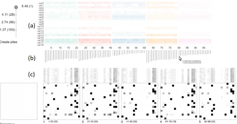
Fig. 4. The two linked views of BayesPiles (a) Overview of 99 networks produced in five runs and shown as summary columns. Different colours indicate different runs. (b) A histogram with the distribution of scores. By hovering over each bar, details such as the computed score value, the run ID and the iteration appear as a tooltip. (c) Initially the consensus pile is empty. Piles 1-5 contain networks from the five different runs and shown using the top-down mode. Opacity encodes the weight of each edge (cell) in piles of superimposed networks. Opacity is also used to summarise the out-degrees which except from the overview also appear at the top edge of each pile.

Visualisation design:In a second period of our design study, we sought for a visualisation idiom which could be successfully applied to the data and support the tasks. We conducted a literature review and we found that matrix representations were more promising compared to node-link diagrams because of their visual scalability and potential for information design. For both representations—node-link and matrices—we discussed visualisation systems and techniques with our collaborators. Eventually we identified MultiPiles as the most promising visualisation technique for the respective type of data (large collections of scored BNs) and our tasks.

Feature iteration:In the third period of our design study we extended MultiPiles to specifically support our analysis tasks in Section2.3. We were following an iterative approach; generating a number of sketches and interactive prototypes, discussing them with our collaborators, and refining our design and features based on their feedback.

3.2 Exploring hundreds of scored directed networks

Fig4shows the interface of BayesPiles with the following views: (a) a heatmap summary view for each network (column) and their node degree (row), (b) bar charts visualising each network’s assessed score, and (c) a detail view of networks grouped in piles, alongside with a placeholder (empty matrix) for the user-created consensus network. The following details each view and the respective interactions.

The first limitation of MultiPiles is that networks have to be in afixed order(time) and piles can

Fig. 5. Directed versus undirected node-link and matrix representations. (a) Node-link representation of a directed network. (b) The same directed network as encoded in top-down mode. Rows encode incoming edges and columns outgoing edges resulting in an adjacency matrix that is not symmetric. (c) The out-degree of each node as encoded using opacity in a summary column. (d) Node-link representation of an undirected network. (e) The undirected network shown in skeleton-mode resulting in a symmetric adjacency matrix (MultiPiles visualisation method). (f) The degree of each node as encoded using opacity in a summary column.

represent directed graphs [50], there are no clear guidelines of how this can be done effectively. Thus, in order to support T1, we were inspired by other approaches [3,11,37] to adopt a top-down directed adjacency matrix representation. Rows indicate incoming edges and columns indicate outgoing edges, resulting in an adjacency matrix which is not symmetric. Fig.5demonstrates how the node-link diagram in (a) is encoded as a top-down directed adjacency matrix in (b). In Fig.5 (b), column 3 shows the four outgoing edges from node 3, while row 3 shows that there are no incoming edges to node 3. In addition to the top-down mode, BayesPiles also supports a skeleton mode which ignores the direction of the edges and shows an undirected adjacency matrix similar to MultiPiles (Fig.5(e)).

When multiple networks are superimposed, opacity encodes the edge weights in the resulting network. These weights provide an indication of how frequently the edge appears in networks present in the pile. Moreover, opacity is used in the column summary of the directed network (Fig.5 (c)) that encodes the out-degree of each node. In skeleton mode, opacity encodes node degree, as the edges are undirected (Fig.5(f)).

A third limitation of MultiPiles is that it does not visualise any data specific to networks, such as a numeric quality score in our case. We hence added value bars at the bottom of each summary column. This encoding is a top-down histogram of network scores which provides an overview of their distribution in the solution space (Fig.4(b)). In order to allow for comparisons between runs, we normalise the bar lengths between the highest and the lowest network score.

3.3 Importing and ordering multiple network collections

Fig. 6. Node reordering improves network comparison and pattern recognition in matrices. (a) Five piles in skeleton mode before applying node reordering. (b) The same five piles after node reordering. It is easier to spot differences such as an edge which is only missing in the second pile from the left (in last row and third column).

important for guiding future heuristic searches and helps users in tuning parameters for improving search results.

Apart from changing the order of the sampled networks, users can also reorder the nodes within the matrices (Fig.6). In general, node reordering is important for effective matrix-based representations of networks and is similar to graph layouts in node-link diagrams [16]. In BayesPiles, node reordering is applied globally to the entire data with all matrices taking the same order. In particular, theoptimal leaf orderingalgorithm is applied which uses hierarchical clustering to place

the most similar rows across all matrices close to each other [13]. Then the ordering of the rows is also applied to the columns. The similarity matrix for each network is calculated using the Manhattan distance. The implementation of this algorithm in JavaScript was found in the library

Reorder.js[23]. Node reordering enables comparisons between matrices and piles and makes it

easier for the users to see differences between runs. It can reveal interesting patterns in the data (Fig.6(b)). At any point, the user can switch back to the original node ordering as provided by the dataset.

BayesPiles also supports the visualisation of multiple collections of BNs, generated by different runs of the heuristic search algorithm. Comparing runs is useful for determining the shape of the solution space more reliably. For instance, if networks appear to approach the same single optimum solution across multiple runs, the analyst would have confidence that the top-scoring network is reproducible and representative of the data, since no other variation is observed in the solution space. When this is the case, the gradual improvement in score is coinciding with the addition of an edge until no more improvement in score is observed. We refer to this pattern as thehill-climbing pattern. However, if multiple runs produce high-scoring networks of different

Comparing high-scoring networks found in different search attempts is important for discovering variation between runs. In order to facilitate comparison, scores are globally normalised and colour used [27] to encode the results of up to 12 different algorithm runs. Results from five runs are shown in Fig.4(a). For a larger number of runs, colours are repeated, but analysts rarely explore the results from more than ten runs simultaneously in our experience. By examining the scores (Fig.4(b)), it becomes clear that only a few runs found substantially high-scoring networks (runs 1, 2 and 4), while the other runs (runs 3 and 5) only found local optima in the search space. This variation in network score between runs indicates a complex solution space with multiple optima for which the construction of a consensus network is required.

3.4 Group and compare networks

Our analysts were interested in exploring and comparing many BNs and found grouping BNs together was important. They were interested in grouping networks of similar score to understand if they belong to the same equivalence class. Networks of the same equivalence class are math-ematically equivalent representations, differing in only the directionality of some (or all) edges. Networks of the same equivalence class have the same score. If many of them are added to the consensus, then it could be a biased result based on the size of the equivalence class rather than the probability of the solution. The histogram can help identify networks of similar scores, but it cannot be used alone to check if the networks belong to the same equivalence class. When there are multiple hills in the dataset, networks of the same score may have very different structure. Therefore, in order to find equivalence classes, it is important to inspect and compare edges and their directionality within groups of networks that have the same score.

The user needs to group BNs of the same score and then needs to identify networks of the same equivalence class within that group. In BayesPiles, the top-down histogram sorted by score can help analysts identify networks of similar score to pile (i.e. group) them together. Piling networks could be automatic by using the dynamic slider provided by MultiPiles, or by manually clicking on the summary view (Fig.4(a)). White vertical lines indicate separate piles. Automatic piling based on score difference is sometimes possible, but identifying a distinctive drop in score is often a question of individual judgement, especially when the solution space has multiple hills. Skeleton mode can help to identify networks that belong to the same equivalence class as these networks have nodes with the same degree. Therefore, their column summaries look the same.

The cover matrix of each pile summarises the networks it contains and enables the interactive comparison of edges within these piles by hovering over their summaries. Edges that exist in all networks appear black in the cover matrix, while lighter shades of grey indicate lower frequency of the edge (Fig.4(c)). In skeleton mode, edges in the cover matrix that belong to the same equivalence class will appear very dark. If many equivalence classes appear in the results, it could mean that the directionality of the edges is not informative. In these cases, it would be preferable to represent these networks ignoring directionality by using skeleton mode.

In the top-down mode, the two directions of an edge are on opposite sides of the diagonal of the matrix, making it difficult to compare opacity levels. Inspecting only one of the edges does not reveal much information about the opacity of the edge that points to the opposite direction because opacities depend on the frequency of the edges in the pile and not on the number of edges that point in the opposite direction.

top-down mode. Depending on the task, analysts can easily switch between the three network representations.

Fig. 7. The evolution of the design for comparing edges of opposite directions. Intermediate design options created ambiguities and visual artefacts because of adjacent neighbouring edges. In the final design (diamond mode), only the (top and bottom) triangles that encode the opposite directions (in and out respectively) appear adjacent.

Our analysts found the diamond design easier to read, compared to other alternatives (Fig.7), because it limited visual artefacts, which could appear due to neighbouring triangles. The users also found intuitive the way directionality is encoded, as the upper and lower triangles could be easily interpreted as arrow heads pointing inwards and outwards the node indicated by each column.

Juxtaposing matrices and piles, as in MultiPiles, can help users to make these comparisons. However, this task becomes more and more difficult as the size or the number of matrices increases. The difficulty is that the user must make a judgement on the opacity of two edges which could be separated in the visualisation.

Fig. 8. Interactively comparing piles. (a) Top-down mode highlights differences in addition and removal of edges. (b) Diamond mode highlights change in direction of edges between piles. In both modes it becomes evident that the hovered consensus pile is more similar to piles 1, 2 and 4 and less similar to piles 3 and 5.

3.5 Graph filtering of nodes and edges

As part of task T4, analysts wanted to focus on a small number of nodes within a network. Even though MultiPiles supports subnetwork selection by dragging the mouse over node labels, our analysts required filtering based on graph connectivity across all matrices and the ability to exclude nodes that are disconnected. Our analysts also wanted to filter edges in the cover matrix based on the percentage of networks in the pile that contain the edge.

To satisfy task T4, we introduced two dynamic sliders [2] that provide edge and node filtering capabilities. Disconnected nodes are automatically filtered out and appear in a list. Node filtering is applied globally based on the overall connectivity of nodes in all networks. Edge filtering, however, is applied locally at a pile level. For instance, when the edge filtering level is set to 50%, all edges that appear in less than half of the networks in each pile are removed from the cover matrix. Setting this slider to 100% will place only those edges that are present in all networks of the pile in the cover matrix, resulting in a logical AND operation. On the contrary, setting this slider to 0% will include all edges in the cover matrix, resulting in a logical OR operation. Depending on the circumstances experts may choose to present a denser network with weaker edges or only show the strong edges for which they are more confident about. Filtering edges provides less information about the results (i.e. content) but also increases confidence about the consistency of the reported edges. Our analysts found this feature particularly useful when deciding which edges should be included in the consensus network because this is a task that requires integration of domain knowledge. According to our users, the final decision for setting the slider depends equally on what is shown on the display and their background knowledge about the system under study. One of our users reported:“if I’m working with a biologist who is planning to do very expensive experiments, one per edge and could only do a handful of experiments, I’d want to give them only 100% edges if I could! Basically, the most confident I could be. Alternatively, if we’re more interested in a holistic view of ’network structure’ including more edges with less confidence would make sense”.

3.6 Viewing outgoing edges of nodes in hundreds of networks

The overview of piled node summaries enables analysts to identify nodes with high out-degree. To better support T5, we extend this feature as analysts were interested in seeing if the same outgoing edges appear in multiple networks for a selected node, as the out-degree may be similar between networks, but the actual edges differ from network to network. Analysts were interested in stable blocks of edges as network scores change. Consistency and variation in edge appearance is important, but these patterns cannot be easily explored in collections of hundreds of networks. Thus, we modified a feature of MultiPiles, which shows all the connections of a node, to present a summary of the outgoing edges for a selected node. By hovering over a node label, all the out-going edges from that node appear for every network and collection in the dataset. An opaque rectangle indicates the existence of an edge from the selected node to another node in the dataset for every network, while blank spaces indicate that no edge is present (Fig.9).

3.7 Manual consensus network construction

Fig. 9. Comparing representations that show the out-going edges from a selected node across a collection of networks. (a) Showing out-going edges from node 3 in 4 networks using a node-link diagram in which networks are superimposed and encoded using different colours. The resulting visualisation is already hard to read and it can hardly scale for few more networks. (b) For the same task, a matrix-based representation, similar to a heatmap, is much more scalable. Opaque rectangles indicate the existence of an edge in a network and blank rectangles indicate its absence. (c) Users can hover over the label of a node (here var16) and all out-going edges will appear in the column summaries across all networks of multiple runs (here there are 99 networks in total). Interesting patterns may appear. For instance, the analyst can observe that the edge from var16 to var6 does not appear in any of the networks found by runs 3 (blue) and 5 (pink).

the piles canvas (bottom linked view) (Fig.2), indicating that it has been added to the consensus network. The selected network will be copied to the consensus pile and can only be added once. Repeating the same interaction on the same network will remove it from the consensus pile. Piles of networks can be also added/removed from the consensus by clicking on a pile at the bottom view.

4 EVALUATION

We evaluated BayesPiles in three case studies with three computational biologists visualising real biological data. The data was explored by our analysts without our presence. In the first two cases, the analysts examined data from experiments conducted and published in previous studies. The purpose of repeating previous experiments was to verify findings, detect inconsistencies, and gain new insights regarding the decision-making process followed during the analysis. This test was the first time that BayesPiles was used under real conditions. In the third case study, network inference had not been previously undertaken by the domain scientist and BayesPiles was used as part of their exploration strategy. In particular, our collaborators wanted to extend their analysis to infer networks. This case study provided an opportunity to assess how BayesPiles can improve the analyst’s workflow in an ongoing experiment.

Two of our analysts were already familiar with BayesPiles as they provided feedback when developing BayesPiles. After a very short training period, they were using it with increased confidence. They performed the analysis of their own data individually and were interviewed afterwards. From these interviews, we collected anecdotal evidence about the effectiveness of our approach and its applicability to computational biology research. A third researcher used BayesPiles to analyse a fourth real dataset of neuroimaging scans, guided by one of our analysts who had experience with BayesPiles. The analysis revealed a hill-climbing pattern, similar to our first case study. Below, we represent only three most representative use cases from our collaborators.

4.1 Use cases

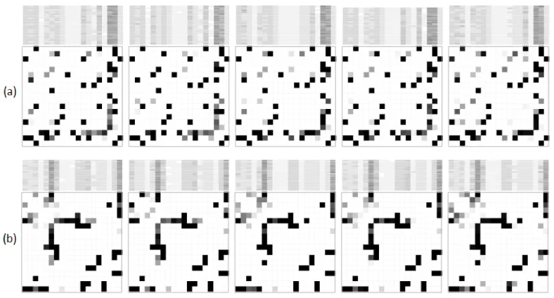
Fig. 10. The hill-climbing pattern consistently appearing in five repetitions of the search. (a) Summary of networks when ordered by score. Networks of the same score are piled. (b) Piles shown in the top-down mode. Fully opaque edges show that all five runs produced identical results. (c) The outgoing edges for var2 look the same across all runs when networks are ordered based on their run ID. A smooth asymptotic curve appears in the histogram of their scores, indicating a hill-climbing pattern.

among these regions [47]. In the original analysis, a greedy search was run and the single top-scoring network presented as the solution. Repeated runs of the algorithm resulted in the same top-scoring network.

Our analyst repeated the original search on one bird’s data and the networks were visualised in BayesPiles. The resulting visualisation showed a smooth, asymptotic increase across all scores, suggesting a single hill-climb. By piling all networks together and scanning the mouse down the pile, or by juxtaposing them as small multiples, the analyst could confirm the hill-climbing pattern. Our analyst made one further check, repeating the search five times and importing them all into BayesPiles. All searches revealed the same asymptotic curve in scores (Fig.10(c)) and the same summary matrix representation, suggesting each search had climbed the same hill. This was confirmed by ordering the networks by score and piling identical scores (Fig.10(a)). The piles showed identical links visible via fully dark squares in the matrix (Fig.10(b)). This finding was also confirmed by hovering on the labels of each node showing that for each run networks had the exact same outgoing edges (Fig.10(c)).

The analyst not only reproduced the results of a previous experiment but also was more confident that selecting the top-scoring network from a greedy search was the correct choice for this dataset. BayesPiles provided a concrete visualisation of the search’s hill-climb, enabling a decision made not solely on reproducibility but instead on a visualisation of the sampled search space.

a consensus across 1000, and used only the links in common from ten such searches. This was somewhat unsatisfactory as almost half the links across all consensus networks were ignored (compare Fig 5 to Fig 7 in [42]), but reproducibility was considered paramount.

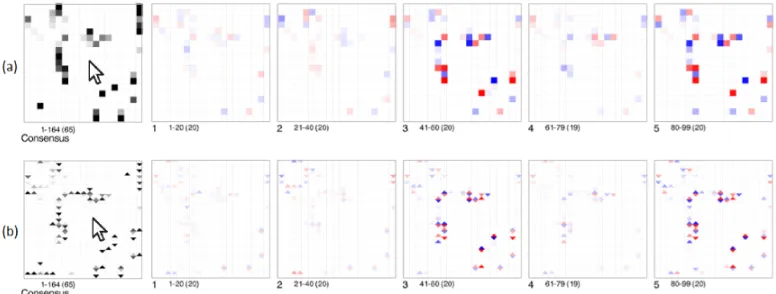
The analyst repeated this experiment in a similar way by beginning with a greedy search but moved immediately onto simulated annealing when BayesPiles revealed many hills in the solution space and vastly different links present in each high-scoring network. Although the analyst decided to follow the same analysis scenario as before, this time, BayesPiles provided the opportunity to explore the solution space of 1000 networks. While only a couple of hundred could appear at the same time on screen, the analyst could use the mouse wheel to scroll through all of them. After sorting them by score, one of the first things that the analyst spotted was that the solution space appeared flat in many areas. However, after a closer look at the networks of the same score this was revealed to not be the case. Skeleton mode revealed that many networks belonged to the same equivalence class (Fig.11(a)), and diamond mode showed that there was high variance in edge direction within and across equivalence classes (Fig.11(b)).

(a) Flat areas in the solution space (b) Diamond mode showing inconsistent directionality of

edges

Fig. 11. (a) The even length of score bars together with the solid opacity of column summaries in skeleton mode suggest that networks 12-45 belong to the same equivalence class. (b) However, using the diamond mode reveals that there is a lot of variation in the directionality of edges within and across piles.

These findings led our analyst to prune networks of the same equivalence class in the parameters and to switch to skeleton mode, ignoring edge directionality. This decision reduced the number of networks considerably, from 1000 to 100. By analysing the solution space of ten runs and using new parameters with a reduced number of networks, our analyst realised that there was still a lot of variation between the high-scoring networks and that scores dropped consistently after the top 20 networks. The analyst decided to ignore lower scoring networks and considered only the top 20 networks from each run. A manual consensus network was constructed from the top-scoring networks using the consensus pile (Fig.2).

pick representative networks with edges which were consistent across runs as shown in Fig.2for networks 120 and 160-164.

Fig. 12. Flexible edge filtering. Users can interactively filter out edges from the consensus network and all other piles. Filtering out edges that appear in less net-works contributes to the construction of a more reliable and reproducible consensus network. In other words, users are enabled to identify and control which edges to include based on how consistently they appear in high-scoring networks.

Finally, edge filtering was used to refine edge selection in the consensus network. The ana-lyst observed that a rate of just over 50% would remove many of the edges from the view. In-stead the analyst decided to include those and only filter out edges that appeared in less than half of the networks (Fig.12). Thus, the analyst achieved to present a consensus network that contained a rich number of edges which were also consistent across runs. In the presentation of the final network, the consistency of each edge is reflected in its opacity.

Without BayesPiles, it would have been dif-ficult to explore all the network structures pro-duced by multiple runs. In the most common scenario, the analyst would simply choose the top-scoring network found by the heuristic

search algorithm (Fig.13(a)). This would produce a very different result when compared to consensus network construction using BayesPiles (Fig.13(c)). Even if the analyst ignored edge directionality (Fig.13(b)), the top-scoring network would still be very different.

Fig. 13. Comparison between the final BN model found by BANJO without BayesPiles with the one con-structed after using BayesPiles. (a) The top-scoring net-work found by BANJO. (b) The same netnet-work shown in skeleton mode. (c) The consensus network constructed manually by the analyst using BayesPiles. Users not only can gain control over the process of consensus network construction but also, they can visualise un-certainties about edges (shown in lower opacity). Note that the fact that the user-created

con-sensus network was different does not neces-sarily mean that it was also better in describing the biological process. The expert user made conscious choices of constructing a different model than the one found before. This was an informed choice that was not possible using purely automatic tools. A rigorous qualitative evaluation with data from an already known biological network will be required in any case.

4.1.3 Gene clusters on ovarian cancer cells. The third dataset consists of expression data of recognised differentially expressed genes in ovarian cancer, in two cell types - one which is responsive to the standard medication regimen, and one which is resistant.

In this ongoing experiment, our analyst initially decided to run a greedy search but

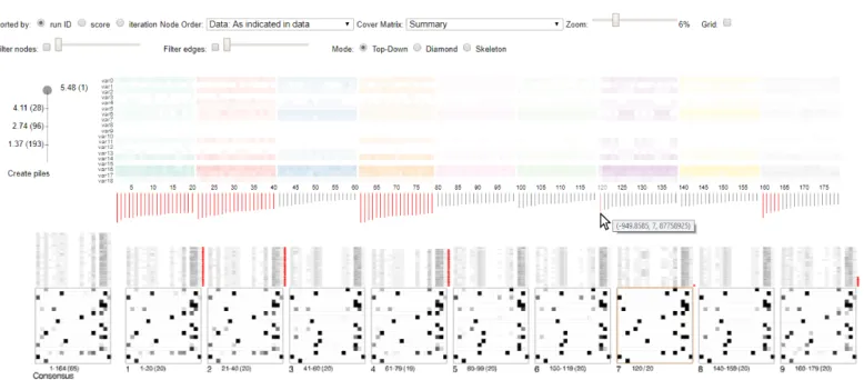
Fig. 14. Results from five search attempts finding Bayesian networks in gene clusters of ovarian cancer cells. (a) User interface controls. (b) A summary of outgoing edges for var41 in five collections of thirty networks each. (c) Networks grouped in five piles and juxtaposed. The column that corresponds to var41 in each pile (manually labelled) appears darker indicating a high out-degree for var41. (d) Differences between the first and the other four runs are shown in the blue and red cells which correspond to edge additions and removals.

connected node (herevar41) (Fig.14(c)) and hovering over its label in Fig.14(b), the analyst sees a

summary of all its outgoing edges in Fig.14(b). From the rather diverse row patterns within each of the coloured columns in Fig.14(b), the analyst found that the particular edges of this node are not consistent; both within the same pile (same colour, same matrix pile) and across runs (different colours, different matrix piles). The lack of consistency across runs was confirmed by hovering over the cover matrix of each pile which showed many differences in red and blue (Fig.14(d)). In other words, the high node degree suggested by the dark colours in the matrices, was resulting from combining the individual networks, which however did not show consistency in their edges. Consequently, the solution space is highly diverse, with many inconsistent edges, which is not clear from the score within BANJO. Given this level of uncertainty the user was not confident enough to report a consensus network before modifying BANJO parameters and repeating the experiment.

It was also clear from the tags under the filter nodes slider (Fig.14(a)) that neither var35, nor var43 have any connections to other nodes and that they have been filtered. The analyst commented:

“Looking at these initial results would definitely lead to me running BANJO on the set, minus variable 43 to see if it has any effect on the overall network. I would also probably, having looked at these results, changed my run to search for a shorter time, or for the consensus graphs to consist of fewer high scoring graphs. Overall, I think this would make the process more efficient.”

4.2 Subjective feedback

analysts work. Generally, all collaborators found that BayesPiles greatly extended their capabilities to explore the data. Below we report on the most prominent remarks. While some of the highlighted aspects refer to features already present in MultiPiles, we see them as evidence of our general approach of adopting MultiPiles to Bayesian network exploration.

Perhaps most important, A3 reported that“You can see theshape of the search space”which

was one of our main goals with BayesPiles.Scalabilitywith respect to the number of individual networks was noted:“I think this method will be of particular use to larger datasets, as it allows for a more instinctive overview of the data and identifies areas or nodes of interest very easily upon first look.” [A1]. On the other hand, interactivity sometimes fell below real-time for datasets around

1000 networks with 50 nodes each. While 1000 is a common size for the data our analysts are dealing with, many other datasets are in the range of several hundreds. We attribute this issue to the fact that BayesPiles (as well as MultiPiles) are currently implemented in WebGL and the relatively prototypical nature of our implementation. Future optimisations could possibly increase scalability further, while keeping the browser-memory limits in mind.

Besides its use of reducing the number of visually present matrices and thus coping with many networks,pilinghas been found to allow for“a quick preview of what a consensus graph would look like and which edges would be prominent, which will hopefully improve the efficiency with which I optimise my BANJO run and therefore save me lots of time”[A1]. The interactive comparison of piles

was found“easy and [happening] in a visual manner” [A1]. It has been found particularly useful

for“understand[ing] which nodes are reliable across runs.” [A1] Another analyst foundinteractive comparison“useful for finding patterns between piles, such as swapping directions.” [A2]. The

manual creation and selection of consensus networkconstruction has been reported as“an extremely valuable new feature [which] allows for a lot more interactive and fluid consensus matrix and will allow removal of any networks that one decides do not better the consensus network. The function is easy to use and understand, especially due to the inclusion of information about which networks are being included and how many. It would be excellent if there was the option to export this manually curated consensus network so it could be used in further study.”[A1]. Export as well as

other common extensions are straightforward and discussed as future work.

Though already part of MultiPiles,reordering nodes and columnshas been regarded an important feature“[aiding] detection of patterns as it allows the main nodes of variation to be focused into one area of the graph[. This makes] it easier to focus on the most important patterns. This new feature definitely highlights for me the benefits of using a visual based method for sorting the networks.”[A1]. On the other hand, in the third case study, the user preferred the original ordering

because they knew that the last set of variables (i.e.nodes) were combinations of treatments and

thus belonged to a different class than the rest of the variables which were gene clusters. Encodings for different classes of variables or an ordering mechanism that distinguishes these classes of variables should be supported in a future version of BayesPiles.

within one image.”[A1]. On the other hand, after not using the system for a period“[it] was hard to remember how the top-down and diamond modes were read[A3]. This could indicate that the glyph

design is not intuitive enough, however the user had only used the system once and it was the first time they could visualise data of this complexity, therefore we believe that regular use will overcome this issue.

Moreover, identifying cycles and other patterns that require following paths is not supported effectively in BayesPiles: “It may be that a biologist may care about cycles in the network, but BayesPiles is to help me to find what to present to the biologist; the visualisation of the final network I present for biological interpretation may be (most likely should be!) done using a different method (e.g., node-link)”[A2]. We designed BayesPiles to support the tasks of the computational biologist

in finding a consensus network. It is clear now that extending the system to support the export of the consensus network for presentation to biologists, would be beneficial. Though we had not designed BayesPiles for presentation scenarios, we believe there is a lot of potential in creating clean visualisations and interactive demos. Along similar lines, one of the analysts commented that

“[v]isualisation can help machine learning (ML) people and users of ML to do a better job in deciding how to guide my search—stay/leave the search area. It helps to learn how the heuristic search works and opens up possibilities in studying heuristic search”[A2]. We take this as evidence for the general

potential of creating visualisation interfaces for biological models.

5 CONCLUSION AND FUTURE WORK

Finding or constructing useful network models plays a pivotal role in understanding how important mechanisms in biological systems work. We introduced BayesPiles, a visual analytics system based on MultiPiles and redesigned for Bayesian networks. BayesPiles allowed our analyst collaborators to better understand the structure of the solution space, to explore, compare and combine network structures, and to construct consensus networks. All these aspects of Bayesian methods producing hundreds of scored directed networks are hard to explore without the aid of visualisation. BayesPiles enables the exploration, organisation and comparison of hundreds of scored directed networks from multiple heuristic search runs. It features two matrix-based representation modes for directed networks (top-down and diamond), a normalised histogram that shows the distribution of scores in the solution space, flexible network ordering based on run ID, iteration or score, node reordering, interactive comparison of networks across groups, support for the manual construction of a consensus network, interactive graph filtering mechanisms and a summary view of all outgoing edges for selected nodes.

showing specific attributes on a network’s links (matrix cells). Regarding scalability, we tested BayesPiles with networks of 44 nodes. In future work, it would be interesting to test its performance and provide additional support for BNs of even larger size. Also, distinguishing between different classes of variables (network nodes) should be supported, providing different visual encodings or a more flexible node reordering mechanism.

We intend to investigate support for the representation and exploration of dynamic Bayesian networks, which result in the comparison of hundreds of dynamic networks. The specific challenges that arise in exploring dynamic Bayesian networks include: how to visualise order, duration, repetition; how to pile (aggregate) sets of dynamic networks, supporting detailed comparison between networks, tracking the evolution of specific edges, and finally filtering and focusing on specific time slices in the respective networks. One possible solution today are superimposed time curves [12], an extension of multi-dimensional scaling. However, time curves give only very high-level changes and do not show any topology.

In summary, our work suggests that more visualisation approaches are required for tackling optimisation problems, in understanding the solution space and how heuristic search works. We believe that this could be a fruitful area in which the two fields of machine learning and visualisation cross borders.

ACKNOWLEDGMENTS

We would like to thank Edinburgh Napier University for funding this PhD work.

REFERENCES

[1] A. Abuthawabeh and D. Zeckzer. 2013. IMMV: An interactive multi-matrix visualization for program comprehension.

In2013 First IEEE Working Conference on Software Visualization (VISSOFT). 1–4.DOI:http://dx.doi.org/10.1109/VISSOFT.

2013.6650549

[2] C. Ahlberg and B. Shneiderman. 1994. Visual information seeking: Tight coupling of dynamic query filters with

starfield displays. InProceedings of the SIGCHI conference on Human factors in computing systems. ACM, 313–317.

[3] B. Alper, B. Bach, N. H. Riche, T. Isenberg, and J. D. Fekete. 2013. Weighted Graph Comparison Techniques for Brain

Connectivity Analysis. InProceedings of the SIGCHI Conference on Human Factors in Computing Systems (CHI ’13).

483–492.DOI:http://dx.doi.org/10.1145/2470654.2470724

[4] K. Andrews, M. Wohlfahrt, and G. Wurzinger. 2009. Visual Graph Comparison. In2009 13th International Conference

Information Visualisation. 62–67. DOI:http://dx.doi.org/10.1109/IV.2009.108

[5] D. Archambault. 2009. Structural Differences Between Two Graphs Through Hierarchies. InProceedings of Graphics

Interface 2009 (GI ’09). Canadian Information Processing Society, Toronto, Ont., Canada, Canada, 87–94. http://dl.acm.

org/citation.cfm?id=1555880.1555905

[6] D. Archambault, H. C. Purchase, and B. Pinaud. 2011.Difference Map Readability for Dynamic Graphs. Springer Berlin

Heidelberg, Berlin, Heidelberg, 50–61.

[7] B. Bach, P. Dragicevic, D. Archambault, C. Hurter, and S. Carpendale. 2016. A Descriptive Framework for Temporal

Data Visualizations Based on Generalized Space-Time Cubes. InComputer Graphics Forum. Wiley Online Library.

[8] B. Bach, N. Henry-Riche, T. Dwyer, T. Madhyastha, J. D. Fekete, and T. Grabowski. 2015. Small MultiPiles: Piling

Time to Explore Temporal Patterns in Dynamic Networks. Computer Graphics Forum34, 3 (2015), 31–40. DOI:

http://dx.doi.org/10.1111/cgf.12615

[9] B. Bach, G. Legostaev, and E. Pietriga. 2010. Visualizing populated ontologies with OntoTrix. InProceedings of the 2010

International Conference on Posters & Demonstrations Track-Volume 658. CEUR-WS. org, 85–88.

[10] B. Bach, E. Pietriga, and J. D. Fekete. 2014. Visualizing dynamic networks with matrix cubes. InProceedings of the 32nd

annual ACM conference on Human factors in computing systems. ACM, 877–886.

[11] B. Bach, E. Pietriga, I. Liccardi, and G. Legostaev. 2011. OntoTrix: A Hybrid Visualization for Populated Ontologies. In

Proceedings of the 20th International Conference Companion on World Wide Web (WWW ’11). ACM, New York, NY,

USA, 177–180. DOI:http://dx.doi.org/10.1145/1963192.1963283

[12] B. Bach, C. Shi, N. Heulot, T. Madhyastha, T. Grabowski, and P. Dragicevic. 2016. Time curves: Folding time to visualize

[13] Z. Bar-Joseph, D. K. Gifford, and T. S. Jaakkola. 2001. Fast optimal leaf ordering for hierarchical clustering.Bioinformatics

17 (2001), S22–S29.DOI:http://dx.doi.org/10.1093/bioinformatics/17.suppl 1.S22

[14] F. Beck, M. Burch, S. Diehl, and D. Weiskopf. 2016. A Taxonomy and Survey of Dynamic Graph Visualization.Computer

Graphics Forum(2016). DOI:http://dx.doi.org/10.1111/cgf.12791

[15] F. Beck and S. Diehl. 2013. Visual comparison of software architectures.Information Visualization12, 2 (2013), 178–199.

DOI:http://dx.doi.org/10.1177/1473871612455983

[16] M. Behrisch, B. Bach, N. H. Riche, T. Schreck, and J. D. Fekete. 2016. Matrix Reordering Methods for Table and Network

Visualization.Computer Graphics Forum(2016). DOI:http://dx.doi.org/10.1111/cgf.12935

[17] S. C. Chan, L. Zhang, H. C. Wu, and K. M. Tsui. 2015. A Maximum A Posteriori Probability and Time-Varying Approach

for Inferring Gene Regulatory Networks from Time Course Gene Microarray Data. IEEE/ACM Transactions on

Computational Biology and Bioinformatics12, 1 (Jan 2015), 123–135. DOI:http://dx.doi.org/10.1109/TCBB.2014.2343951

[18] C. Chang, B. Bach, T. Dwyer, and K. Marriott. 2017. Evaluating Perceptually Complementary Views for Network

Exploration Tasks. InProceedings of the 2017 CHI Conference on Human Factors in Computing Systems. ACM, 1397–1407.

[19] D. M. Chickering. 1996.Learning Bayesian Networks is NP-Complete. Springer New York, New York, NY, 121–130.

DOI:http://dx.doi.org/10.1007/978-1-4612-2404-4 12

[20] G. F. Cooper. 1990. The computational complexity of probabilistic inference using bayesian belief networks.Artificial

Intelligence42, 2 (1990), 393 – 405. DOI:http://dx.doi.org/10.1016/0004-3702(90)90060-D

[21] M. Cossalter, O. J. Mengshoel, and T. Selker. 2011. Visualizing and understanding large-scale Bayesian networks. In

The AAAI-11 Workshop on Scalable Integration of Analytics and Visualization.

[22] J. Ellson, E. Gansner, L. Koutsofios, S. C. North, and G. Woodhull. 2002.Graphviz— Open Source Graph Drawing Tools.

Springer Berlin Heidelberg, Berlin, Heidelberg, 483–484. DOI:http://dx.doi.org/10.1007/3-540-45848-4 57

[23] J. D. Fekete. 2015. Reorder.js: A JavaScript Library to Reorder Tables and Networks. IEEE VIS 2015. (Oct. 2015).

https://hal.inria.fr/hal-01214274Poster.

[24] M. Freire, C. Plaisant, B. Shneiderman, and J. Golbeck. 2010. ManyNets: an interface for multiple network analysis

and visualization. InProceedings of the SIGCHI Conference on Human Factors in Computing Systems. ACM, 213–222.

[25] M. Ghoniem, J. D. Fekete, and P. Castagliola. 2004. A Comparison of the Readability of Graphs Using Node-Link and

Matrix-Based Representations. InIEEE Symposium on Information Visualization. 17–24. DOI:http://dx.doi.org/10.1109/

INFVIS.2004.1

[26] M. Gleicher, D. Albers, R. Walker, I. Jusufi, C. D. Hansen, and J. C. Roberts. 2011. Visual comparison for information

visualization.Information Visualization10, 4 (2011), 289–309.

[27] M. Harrower and C. A. Brewer. 2003. ColorBrewer. org: an online tool for selecting colour schemes for maps.The

Cartographic Journal40, 1 (2003), 27–37.DOI:http://dx.doi.org/10.1179/000870403235002042

[28] M. Hasco¨et and P. Dragicevic. 2012. Interactive graph matching and visual comparison of graphs and clustered graphs.

InProceedings of the International Working Conference on Advanced Visual Interfaces. ACM, 522–529.

[29] M. Hecker, S. Lambeck, S. Toepfer, E. van Someren, and R. Guthke. 2009. Gene regulatory network inference: Data

integration in dynamic models - A review.Biosystems96, 1 (2009), 86 – 103.DOI:http://dx.doi.org/10.1016/j.biosystems.

2008.12.004

[30] D. Heckerman, D. Geiger, and D. M. Chickering. 1995. Learning Bayesian networks: The combination of knowledge

and statistical data.Machine Learning20, 3 (1995), 197–243. DOI:http://dx.doi.org/10.1007/BF00994016

[31] S. M. Hill, L. M. Heiser, T. Cokelaer, M. Unger, N. K. Nesser, D. E. Carlin, Y. Zhang, A. Sokolov, E. O. Paull, C. K. Wong, and others. 2016. Inferring causal molecular networks: empirical assessment through a community-based effort.

Nature methods13, 4 (2016), 310–318.DOI:http://dx.doi.org/doi:10.1038/nmeth.3773

[32] D. Husmeier. 2003. Sensitivity and specificity of inferring genetic regulatory interactions from microarray

exper-iments with dynamic Bayesian networks. Bioinformatics19, 17 (2003), 2271–2282. DOI:http://dx.doi.org/10.1093/

bioinformatics/btg313

[33] N. Kadaba, P. Irani, and J. Leboe. 2007. Visualizing Causal Semantics Using Animations. IEEE Transactions on

Visualization and Computer Graphics13, 6 (Nov 2007), 1254–1261. DOI:http://dx.doi.org/10.1109/TVCG.2007.70528

[34] D. Koller and N. Friedman. 2009.Probabilistic graphical models: principles and techniques. MIT press.

[35] B. K. Kuntal, A. Dutta, and S. S. Mande. 2016. CompNet: a GUI based tool for comparison of multiple biological

interaction networks.BMC Bioinformatics17, 1 (2016), 185.DOI:http://dx.doi.org/10.1186/s12859-016-1013-x

[36] C. Lacave, M. Luque, and F. J. Diez. 2007. Explanation of Bayesian Networks and Influence Diagrams in Elvira.

IEEE Transactions on Systems, Man, and Cybernetics, Part B (Cybernetics)37, 4 (Aug 2007), 952–965. DOI:http:

//dx.doi.org/10.1109/TSMCB.2007.896018

[37] I. Liiv. 2010. Seriation and matrix reordering methods: An historical overview.Statistical Analysis and Data Mining3,

2 (2010), 70–91. DOI:http://dx.doi.org/10.1002/sam.10071

[38] J. Linde, S. Schulze, S. G. Henkel, and R. Guthke. 2015. Data-and knowledge-based modeling of gene regulatory

[39] D. J. Lunn, A. Thomas, N. Best, and D. Spiegelhalter. 2000. WinBUGS - A Bayesian modelling framework: Concepts,

structure, and extensibility.Statistics and Computing10, 4 (01 Oct 2000), 325–337. DOI:http://dx.doi.org/10.1023/A:

1008929526011

[40] J. Mackinlay. 1986. Automating the Design of Graphical Presentations of Relational Information.ACM Trans. Graph.5,

2 (April 1986), 110–141. DOI:http://dx.doi.org/10.1145/22949.22950

[41] D. Marbach, J. C. Costello, R. K¨uffner, N. M. Vega, R. J. Prill, D. M. Camacho, K. R. Allison, M. Kellis, J. J. Collins, G.

Stolovitzky, and others. 2012. Wisdom of crowds for robust gene network inference. Nature methods9, 8 (2012),

796–804.DOI:http://dx.doi.org/doi:10.1038/nmeth.2016

[42] F. Matth¨aus, V. A. Smith, A. Fogtman, W. H. Sommer, F. Leonardi-Essmann, A. Lourdusamy, M. A. Reimers, R. Spanagel, and P. J. Gebicke-Haerter. 2009. Interactive molecular networks obtained by computer-aided conversion of microarray

data from brains of alcohol-drinking rats.Pharmacopsychiatry42, S 01 (2009), S118–S128.

[43] T. Munzner. 2009. A nested model for visualization design and validation.Visualization and Computer Graphics, IEEE

Transactions on15, 6 (2009), 921–928.

[44] R. Sadana, T. Major, A. Dove, and J. Stasko. 2014. OnSet: A Visualization Technique for Large-scale Binary Set Data.

IEEE Transactions on Visualization and Computer Graphics20, 12 (Dec 2014), 1993–2002. DOI:http://dx.doi.org/10.

1109/TVCG.2014.2346249

[45] M. H. Schulz, W. E. Devanny, A. Gitter, S. Zhong, J. Ernst, and Z. Bar-Joseph. 2012. DREM 2.0: Improved reconstruction

of dynamic regulatory networks from time-series expression data. BMC Systems Biology6, 1 (2012), 104. DOI:

http://dx.doi.org/10.1186/1752-0509-6-104

[46] M. Sedlmair, M. Meyer, and T. Munzner. 2012. Design study methodology: Reflections from the trenches and the

stacks.Visualization and Computer Graphics, IEEE Transactions on18, 12 (2012), 2431–2440.

[47] V. A. Smith, J. Yu, T. V Smulders, A. J Hartemink, and E. D. Jarvis. 2006. Computational Inference of Neural Information

Flow Networks.PLOS Computational Biology2, 11 (11 2006), 1–14.DOI:http://dx.doi.org/10.1371/journal.pcbi.0020161

[48] M. E. Smoot, K. Ono, J. Ruscheinski, P. L. Wang, and T. Ideker. 2011. Cytoscape 2.8: new features for data integration

and network visualization.Bioinformatics27, 3 (2011), 431–432.DOI:http://dx.doi.org/10.1093/bioinformatics/btq675

[49] A. Vogogias, J. Kennedy, D. Archambault, V. A. Smith, and H. Currant. 2016. MLCut: Exploring Multi-Level Cuts in

Dendrograms for Biological Data. InComputer Graphics and Visual Computing (CGVC), Cagatay Turkay and Tao Ruan

Wan (Eds.). The Eurographics Association. DOI:http://dx.doi.org/10.2312/cgvc.20161288

[50] T. von Landesberger, A. Kuijper, T. Schreck, J. Kohlhammer, J. J. van Wijk, J. D. Fekete, and D. W. Fellner. 2011. Visual

Analysis of Large Graphs: State-of-the-Art and Future Research Challenges.Computer Graphics Forum30, 6 (2011),

1719–1749.DOI:http://dx.doi.org/10.1111/j.1467-8659.2011.01898.x

[51] J. Wang and K. Mueller. 2016. The Visual Causality Analyst: An Interactive Interface for Causal Reasoning. IEEE

Transactions on Visualization and Computer Graphics22, 1 (Jan 2016), 230–239. DOI:http://dx.doi.org/10.1109/TVCG.

2015.2467931

[52] Y. Yang, T. Dwyer, S. Goodwin, and K. Marriott. 2017. Many-to-Many Geographically-Embedded Flow Visualisation:

An Evaluation. IEEE Transactions on Visualization and Computer Graphics23, 1 (Jan 2017), 411–420. DOI:http:

//dx.doi.org/10.1109/TVCG.2016.2598885

[53] A. Yates, A. Webb, M. Sharpnack, H. Chamberlin, K. Huang, and R. Machiraju. 2014. Visualizing Multidimensional

Data with Glyph SPLOMs.Computer Graphics Forum33, 3 (2014), 301–310.DOI:http://dx.doi.org/10.1111/cgf.12386

[54] W. C. Young, A. E. Raftery, and K. Y. Yeung. 2014. Fast Bayesian inference for gene regulatory networks using ScanBMA.

BMC Systems Biology8, 1 (2014), 47. DOI:http://dx.doi.org/10.1186/1752-0509-8-47

[55] J. D. Zapata-Rivera, E. Neufeld, and J. E. Greer. 1999. Visualization of Bayesian Belief Networks. InIEEE Visualization

1999 Late Breaking Hot Topics Proceedings. Press, 85–88.