(will be inserted by the editor)
Multigrid algorithms for
hp
-version Interior Penalty
Discontinuous Galerkin methods on polygonal and
polyhedral meshes
P. F. Antonietti · P. Houston · X. Hu · M. Sarti · M. Verani
the date of receipt and acceptance should be inserted later
Abstract In this paper we analyze the convergence properties of two-level and W-cycle multigrid solvers for the numerical solution of the linear system of equa-tions arising from hp-version symmetric interior penalty discontinuous Galerkin discretizations of second-order elliptic partial differential equations on polygo-nal/polyhedral meshes. We prove that the two-level method converges uniformly with respect to the granularity of the grid and the polynomial approximation degree p, provided that the number of smoothing steps, which depends on p, is chosen sufficiently large. An analogous result is obtained for the W-cycle multigrid algorithm, which is proved to be uniformly convergent with respect to the mesh size, the polynomial approximation degree, and the number of levels, provided the number of smoothing steps is chosen sufficiently large. Numerical experiments are presented which underpin the theoretical predictions; moreover, the proposed
Paola F. Antonietti has been partially supported by SIR (Scientific Independence of young Researchers) starting grant n. RBSI14VT0S “PolyPDEs: Non-conforming polyhedral finite element methods for the approximation of partial differential equations” funded by the Italian Ministry of Education, Universities and Research (MIUR).
P. F. Antonietti·M. Sarti·M. Verani
MOX-Laboratory for Modeling and Scientific Computing, Dipartimento di Matematica, Po-litecnico di Milano, Piazza Leondardo da Vinci 32, 20133 Milano, Italy.
P. F. Antonietti
E-mail: [email protected]
M. Sarti
E-mail: [email protected]
M. Verani
E-mail: [email protected]
P. Houston
School of Mathematical Sciences, University of Nottingham, University Park, Nottingham, NG7 2RD, United Kingdom.
E-mail: [email protected]
X. Hu
Department of Mathematics, Tufts University, 503 Boston Avenue Bromfield-Pearson, Med-ford, MA 02155
multilevel solvers are shown to be convergent in practice, even when some of the theoretical assumptions are not fully satisfied.
Keywords hp-discontinuous Galerkin methods· polygonal/polyhedral grids · two-level and multigrid algorithms
Mathematics Subject Classification (2000) 65N30·65N55·65N22
1 Introduction
The original articles concerned with the construction and mathematical analysis of Discontinuous Galerkin (DG) methods date back over 50 years ago. For hyperbolic partial differential equations, in 1973 Reed & Hill, cf. [53], developed the first DG discretization of the neutron transport equation. Independently, DG methods were constructed for elliptic problems based on weakly enforcing Dirichlet boundary conditions; see, for example, [18, 19, 47, 50]. In particular, we highlight the works of Nitsche [50], Baker [20], Wheeler [61] and Arnold [16], which form the basis of the class of interior penalty DG methods. Since the very early work, DG methods were partially abandoned, in part due to the increase in the number of degrees of freedom compared, for instance, with their conforming counterparts. However, in the last two decades there has been a renewed interest in the field of discontinu-ous discretizations both from a theoretical and computational viewpoint, cf. [38, 45, 54, 39], for example. This resurgence is due to the inherent advantages offered by DG schemes, such as, for example, the limited interelement communication, which is restricted only to neighbouring elements, the local conservativity prop-erty, the simplicity in treating meshes with hanging nodes, and the development of efficienthp-adaptivity refinement strategies. Moreover, recently in [21–23, 36] it has been shown that the underlying DG polynomial bases may be efficiently con-structed in the physical frame, without needing to map local polynomial spaces defined in a given reference/canonical frame. In this way, DG methods can easily deal with general-shaped elements, including polygonal/polyhedral elements, cf. [4, 3, 8, 36, 21, 35, 6, 33, 34] and the recent review paper [5]. The flexibility of DG methods in handling general meshes has no immediate counterpart in the con-forming framework, where the design of suitable finite element spaces for meshes of polygons/polyhedra is far from being a trivial task. Several examples include the Composite Finite Element Method [44, 43], the Polygonal Finite Element Method [58, 59], the Extended Finite Element Method [40], the Mimetic Finite Difference Method [46, 32, 30, 31, 28, 7] and the most recent Virtual Element Method [25–27, 1, 2].
physical framework makes the choice of multilevel schemes natural. The flexibility afforded by this approach allows us to define the set of grids needed in the multigrid algorithm by agglomeration; thereby, the definition of the associated subspaces is straightforward, since inter-element continuity is not required. This property overcomes the usual difficulties encountered in the construction of agglomeration multigrid schemes in the conforming framework, where the agglomeration strategy must be followed by a proper definition of the conforming subspaces. In [37], for example, the sublevels are obtained by combining a graph based agglomeration algorithm and re-triangulations, thus resulting in a set of non-nested grids, while the associated nested subspaces are defined by introducing suitable interpolation operators. The resulting V-cycle multigrid algorithm converges uniformly with respect to the meshsizehprovided that the number of levels is kept fixed.
In this paper we analyze the convergence of a two-level scheme and W-cycle multigrid method for the solution of the linear system of equations arising from thehp-version of the interior penalty DG scheme on polygonal/polyhedral meshes [36], thereby, extending the theoretical framework developed in [13] for standard quasi-uniform triangular/quadrilateral meshes, cf. also [14] for three-dimensional numerical experiments. Our analysis is based on the smoothing and approxima-tion properties associated with the proposed method: the former corresponds to a Richardson iteration, whose study requires a result concerning the spectral prop-erties of the stiffness matrix, while the latter is inherent to the interior penalty DG scheme itself and exploits the error estimates derived in [36]. We show that, under suitable assumptions on the agglomerated coarse grid, both the two-level and the W-cycle multigrid schemes converge uniformly with respect to the granularity of the underlying partition and the polynomial approximation degreep, provided that the number of smoothing steps is chosen of orderp2+µ, withµ= 0,1. Throughout the analysis, we also track the dependence of the error reduction factor of the two solvers on the geometric properties of the agglomerated grids, thereby recov-ering a similar result to the case when standard quasi-uniform triangular and/or quadrilateral meshes are employed.
The rest of this paper is organized as follows. In Section 2 we introduce the interior penalty DG scheme for the discretization of second-order elliptic problems on general meshes consisting of polygonal/polyhedral elements. Then in Section 3, we recall some preliminary analytical results concerning this class of schemes. In Section 4 we define the multilevel framework and introduce several technical results. We then focus first on the analysis of the two-level method, followed by the extension to the W-cycle multigrid solver. The main theoretical results are investigated through a series of numerical experiments presented in Section 6, where we also present a comparison with an unsmoothed Algebraic Multigrid method. Finally, in Section 7 we draw some conclusions.
2 Model problem and discretization
We consider the weak formulation of the Poisson problem, subject to a homoge-neous Dirichlet boundary condition: findu∈V =H2(Ω)∩H01(Ω) such that
Z Ω
∇u· ∇v dx=
Z Ω
with Ω ∈ Rd, d = 2,3, a convex polygonal/polyhedral domain with Lipschitz boundary andf a given function inL2(Ω).
For the sake of brevity, throughout this article, we write x.y andx&yin lieu ofx≤Cy andx≥Cy, respectively, for a positive constantC independent of the discretization parameters. Moreover, x≈y means that there exist constants C1, C2>0 such thatC1y≤x≤C2y. When required, the constants will be written explicitly.
In view of the forthcoming multigrid analysis, we denote by{Tj}Jj=1a sequence of partitions of the domain Ω, each of which consists of disjoint open polygo-nal/polyhedral elements κof diameter hκ, such that Ω= S
κ∈Tjκ¯, j = 1, . . . , J.
We denote the mesh size of Tj, j = 1, . . . , J, by hj = maxκ∈Tjhκ. To each Tj, j = 1, . . . , J, we associate the corresponding DG finite element space Vj, j= 1, . . . , J, defined as
Vj ={v∈L2(Ω) :v|κ∈ Ppj(κ), κ∈ Tj},
where Ppj(κ) denotes the space of polynomials of total degree at most pj ≥1 on
κ∈ Tj. A suitable choice of the sequences{Tj}Jj=1 and{Vj}
J
j=1 leads to the so-calledh- andp-multigrid schemes. In particular, theh−multigrid method is based on employing a constant polynomial approximation degree for eachj,j= 1, . . . , J, (i.e.,pj=p), on a set of nested partitions{Tj}Jj=1, such that the coarse levelTj−1,
j= 2, . . . , J, is obtained by agglomeration from Tj in such a way that
hj−1.hj ≤hj−1 ∀j= 2, . . . , J, (2)
i.e., we assume a bounded variation hypothesis between subsequent levels. In the p-multigrid method, the partition is kept fixed for any j, j = 1, . . . , J, while we assume that the polynomial degrees vary moderately from one level to another,
i.e.,
pj−1≤pj.pj−1 ∀j= 2, . . . , J. (3) Note that with the above choices we obtain nested finite element spaces Vj, j= 1, . . . , J,i.e.,V1⊆V2⊆ · · · ⊆VJ.
2.1 Grid assumptions
We denote byFjthe set of all mesh faces; moreover, we have thatFj=FjI∪ FjB, where FjI is the set of interior element faces ofTj, such thatF ⊆∂κ+∩∂κ− for anyF ∈ FjI, whereκ± are two adjacent elements in Tj. The setFjB contains the boundary element faces,i.e.,F ⊂∂Ωfor F∈ FjB.
We are now ready to introduce the following assumptions on the partitionsTj, j= 1, . . . , J; cf. [33]. In the case of theh-multigrid scheme, these assumptions must be satisfied for the meshes generated by the underlying agglomeration process.
Assumption 1 Given κ ∈ Tj, there exists a set of nonoverlapping (not necessarily
shape-regular) d–dimensional simplices T` ⊆ κ, ` = 1,2, . . . , nκ, such that, for any
faceF ⊂∂κ, F=∂κ∩∂T`, for some`,
∪nκ
`=1T`⊆κ,
and the diameterhκ ofκcan be bounded by
hκ. d|T`|
|F| , `= 1,2, . . . , nκ.
Remark 1 We point out that Assumption 1 does not put a restriction on either the number of faces that an element possesses, or indeed the measure of a face of an element κ∈ Tj, relative to the measure of the element itself. This will be particularly important in the agglomeration procedure employed within our h -multigrid method, since as the number of levels increases, the number of faces that the resulting agglomerated elements may contain grows, while their measure, relative to the element measure, may degenerate.
Remark 2 As pointed out in [33], meshes obtained by agglomeration of a finite number of polygons that are uniformly star-shaped with respect to the largest inscribed ball will automatically satisfy Assumption 1. Therefore, from the prac-tical point of view, given a fine-level meshTJ consisting of uniformly star-shaped elements, a finite number of agglomeration steps will produce a sequence of admis-sible grids. To allow the number of agglomeration levels to increase arbitrarily one can eitheri)ensure that each of the agglomerated meshes satisfy Assumption 1;ii)
check, at each level, that the (slightly more restrictive) shape-regularity criterion on the agglomerates is satisfied.
Assumption 2 For any κ ∈ Tj, j = 1, . . . , J, we assume that hdκ ≥ |κ|&hdκ, with d= 2,3.
We next introduce the following additional mesh condition, cf. [35], which will be required in order to obtain the inverse estimates presented in Lemma 4.
Assumption 3 Every polytopic element κ ∈ Tj, admits a sub-triangulation into at
mostmκ∈N non-overlapping, shape-regular simplicessi,i= 1,2, . . . , mκ, such that ¯
κ=∪mκ
i=1¯si and
|si|&|κ|
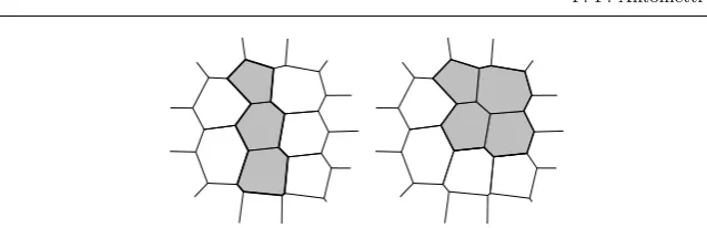
Fig. 1 Examples of agglomerated elements. The agglomerated element on the left violates Assumption 5 whereas the one on the right satisfies Assumption 5.
In view of the approximation result that will be presented in the next section we also introduce the following additional assumption.
Assumption 4 Let Tj]={K}, denote a covering ofΩconsisting of shape-regulard -dimensional simplices K. We assume that, for anyκ∈ Tj, there exists K ∈ Tj] such
thatκ⊂ K,diam(K).hκ, and
max κ∈Tj
cardnκ0∈ Tj:κ0∩ K 6=∅, K ∈ Tj] such that κ⊂ K o
.1.
We also need the following assumption on the quality of agglomerated grids.
Assumption 5 For anyF ∈ Fj∩ Fj−1,j= 2, . . . , J, we denote byκ±j andκ
±
j−1 the
neighboring elements sharing the faceF inTj andTj−1, respectively. We assume that
there existsΘ >0such that
1< hκ±
j−1 hκ±
j
≤Θ ∀F ∈ Fj∩ Fj−1.
We remark that Assumption 5 is satisfied if the agglomeration algorithm pre-serves the shape-regularity of the elements. In Figure 1, we show two examples of possible macroelements: the agglomerate on the left is not suitable to guarantee Assumption 5 due to the presence of a dominant dimension, while the element on the right can be considered appropriate. Moreover, we note that the fulfilment of Assumption 5 can be considered a good criterion in evaluating the quality of the agglomerated grids employed in the multigrid algorithm, cf. Figure 1 for an illustration.
Finally, to keep the notation as simple as possible, in the forthcoming analysis we will assume that, for anyj= 1, . . . , J, the decompositionsTjare quasi-uniform.
Assumption 6 For any j= 1, . . . , J, it holdshj≈minκ∈Tjhκ.
[image:6.595.79.398.73.176.2]2.2 DG formulation
The definition of the proceeding DG method is based on employing suitable jump and average operators. To this end, for (sufficiently smooth) vector- and scalar-valued functionsτ andv, respectively, we define jumps and averages acrossF∈ Fj, j= 1, . . . , J, as follows:
JτK=τ +·
n++τ−·n−, {{τ}}= τ ++τ−
2 , F ∈ F
I j,
JvK=v +
n++v−n−, {{v}}= v ++v−
2 , F ∈ F
I j,
JvK=v +
n+, {{τ}}=τ+, F∈ FjB,
wherev±andτ± denote the traces ofvandτ onF taken from the interior ofκ±, respectively, andn±the outward unit normal vectors to∂κ±, respectively, cf. [17]. On any level j,j = 1, . . . , J, we consider the bilinear form Aj(·,·) :Vj×Vj →R, corresponding to the symmetric interior penalty DG method, defined by
Aj(u, v) = X κ∈Tj
Z κ
∇u· ∇v dx− X
F∈Fj
Z F
({{∇u}} ·JvK+JuK· {{∇v}}) ds
+ X
F∈Fj
Z F
σjJuK·JvKds, (4)
whereσj ∈L∞(Fj) denotes the interior penalty stabilization functionσj :Fj→R+, which is defined by
σj(x) =
Cσj max κ∈{κ+,κ−}
np2j hκ
o
, x∈F, F∈ FjI, F⊂∂κ+∩∂κ−,
Cσj p2j
hκ, x∈F, F ∈ F
B
j , F ⊂∂κ+∩∂Ω,
(5)
withCσj >0 independent ofpj,|F|and|κ|.
In this article, we develop two-level and W-cycle multigrid schemes to compute the solution of the following problem on the finest levelJ: finduJ ∈VJ such that
AJ(uJ, vJ) = Z
Ω
f vJ dx ∀vJ∈VJ. (6)
3 Preliminary results
We first recall the following trace-inverse inequality for polygonal/polyhedral ele-ments.
Lemma 1 Assume that the sequence of meshes Tj, j = 1, . . . , J, satisfies
Assump-tion 1. Letκ∈ Tj, j= 1, . . . , J, be a polygonal/polyhedral element, then the following
bound holds
kvk2L2(∂κ)≤C j inv
p2j hκkvk
2
L2(κ) ∀v∈ Ppj(κ), (7)
The proof can be obtained with trivial modifications with respect to the ones given in [33, 34]. For the sake of completeness we report it and refer to [33, 34] for further details.
Proof From Assumption 1, there exists a set of nonoverlapping (not necessarily shape-regular) d-simplicial elements T` ⊆ κ such that, given a face F ⊂ ∂κ, for some`, 1≤`≤nκ,F =∂κ∩∂T`. Therefore,
kuk2L2(∂κ)= X F⊂∂κ
kuk2L2(F).p2j nκ
X `=1
|F| |T`|
kuk2L2(T
`).
p2j hκ
nκ
X `=1
kuk2L2(T
`)≤
p2j hκkuk
2
L2(κ),
as required. Here, in the first inequality we have employed the following classical trace-inverse estimate ond-simplicial elements
kuk2L2(F).p2j
|F| |T`|
kuk2L2(T
`),
cf. [56, 41], for example; the second bound exploits Assumption 1, namely, that |F||T`|−1.dh−κ1.
Next, we endow the finite element spaces Vj,j= 1, . . . , J, with the following DG norm:
kwk2DG,j = X κ∈Tj
Z κ
|∇w|2 dx+ X F∈Fj
Z F
σj|JwK|2 ds.
The well–posedness of the DG formulation is established in the following lemma
Lemma 2 Assume that the sequence of meshes Tj, j = 1, . . . , J, satisfies
Assump-tion 1 and that the constant Cσj, j = 1, . . . , J, appearing in the definition (5)of the
stabilization function is chosen sufficiently large. Then, the following continuity and coercivity bounds, respectively, hold
Aj(u, v)≤CcontkukDG,jkvkDG,j ∀u, v∈Vj,
Aj(u, u)≥Ccoerkuk2DG,j ∀u∈Vj, (8)
whereCcont andCcoer are positive constants, independent of the discretization
param-eters.
The proceeding error estimates are based on the following approximation re-sult, which is a simplified version of the analogous bound presented in [36, Proof of Theorem 5.2]. To this end, we define E :Hs(Ω)→Hs(Rd),s∈N0, such that Ev|Ω=v, to denote the extension operator presented in Stein [57].
Lemma 3 Assume that Assumptions 1 and 4 hold. Letv|κ ∈Hk(κ), k > d/2, such
thatEv|K∈Hk(K), for eachκ∈ Tj,j= 1, . . . , J, whereκ⊂ K,K ∈ Tj]. Then there
exists a projection operatorΠje :L2(Ω)→Vj such that
kv−Π˜jvkDG,j≤Cjinterp hsj−1
pkj−1−µ/2
kvkHk(Ω), (9)
where s = min{pj + 1, k}, and the constant Cjinterp depends on the shape-regularity constant of the covering Tj], but is independent of the discretization parameters, as well as the number of faces per element and the relative measure of the faces. Here,
Next, we state error bounds for the underlying interior penalty DG scheme in terms of both the DG andL2(Ω)-norms.
Theorem 7 Assume that Assumptions 1 and 4 hold. Denote byuj∈Vj,j= 1, . . . , J,
the DG solution of problem(6)posed on levelj,i.e.,
Aj(uj, vj) = Z
Ω
f vj dx ∀vj∈Vj.
If the solutionuof (1)satisfiesu|κ∈Hk(κ), k >1 +d/2, such that Eu|K∈Hk(K),
for eachκ∈ Tj,j= 1, . . . , J, where κ⊂ K,K ∈ Tj], then the following bounds hold
ku−ujkDG,j≤Gj hsj−1
pkj−1−µ/2
kukHk(Ω), (10)
ku−ujkL2(Ω)≤Cj L2
hsj
pkj−µk
ukHk(Ω), (11)
where s= min{pj+ 1, k}and the constants Gj and CjL2 are independent of the
dis-cretization parameters. Here, µ = 0 whenever a p−optimal interpolant can be con-structed andµ= 1otherwise.
Before proceeding with the proof, we point out that the above error bounds hold provided Assumptions 1 and 4 are satisfied; however, we stress that no limitation is placed on the maximum number of faces that each polygonal/polyhedral element may possess. Moreover, there is no restriction on the relative size of each face of an element compared to its diameter.
Proof The error bound (10) stems from the general result derived in [36, Theo-rem 5.2] under the condition that Assumptions 1 and 4 hold. Thereby, we now proceed with the proof of the bound on theL2(Ω)-norm of the error, cf. (11). To this end, we employ a standard duality argument: let w∈ V, be the solution of the problem
Aj(v, w) = Z
Ω
(u−uj)v dx ∀v∈V,
j= 1, . . . , J. Exploiting a standard elliptic regularity assumption, we note that
kwkH2(Ω).ku−ujkL2(Ω).
According to Galerkin orthogonality, we immediately obtain
ku−ujk2L2(Ω)=Aj(u−uj, w)
=Aj(u−uj, w−wI)
.ku−ujkDG,jkw−wIkDG,j
for allwI ∈Vj. Hence, selectingwI = ˜Πjw, employing (9) gives
kw−wIkDG,j.Cjinterp hj
p1j/2
kwkH2(Ω).Cj interp
hj
p1j−µ/2
ku−ujkL2(Ω),
Equipped with Assumption 3, we now quote the following result from [35]; for brevity the proof is omitted. However, we point out that the proof presented in [35] holds under slightly weaker mesh conditions; for simplicity of presentation, this level of detail is omitted.
Lemma 4 Assume that Assumptions 2 and 3 hold. Then, for anyv∈Vj,j= 1, . . . , J, the following inverse estimate holds
k∇uk2L2(κ)≤C j Ip
4
jh−κ2kuk2L2(κ),
whereCjI >0is independent of the discretization parameters.
The inverse estimate presented in Lemma 4 is fundamental to the proof of the following upper bound on the maximum eigenvalue ofAj(·,·). We recall that the analogous result on standard grids can be found in [10], cf. also [11].
Theorem 8 Given that Assumptions 1, 2, 3, and 6 hold, then for any u ∈ Vj,
j= 1, . . . , J, we have that
Aj(u, u)≤Cjeig p4j h2jkuk
2
L2(Ω),
where the constantCjeig is independent of the discretization parameters.
Proof Given the continuity of the bilinear forms Aj(·,·) stated in Lemma 2, we restrict ourselves to estimate the two terms involved in the DG norm. The local contributions of theH1 seminorm can be simply bounded by applying Lemma 4 and the quasi-uniformity of the partition,i.e.,
X κ∈Tj
|u|2H1(κ)≤ X κ∈Tj
CjIp4jh−κ2kuk2L2(κ)≤
max κ∈Tj
CjI p4
j h2
j
kuk2L2(Ω).
To bound the norm of the jump acrossF ∈ Fj, we employ the inverse inequality (7); thereby, we get
X F∈Fj
kσ1j/2JuKk2L2(F). X κ∈Tj
kσj1/2JuKkL22(∂κ). CσjCjinv p4j h2
j
kuk2L2(Ω).
The statement of the theorem immediately follows based on summing the above bounds.
The theoretical results derived in this section form the basis of the analysis of the proposed multigrid algorithms presented in the following section.
4 Two-level and W-cycle multigrid algorithms
Algorithm 1Two-level scheme Pre-smoothing:
fori= 1, . . . , m1do
z(i)=z(i−1)+B−1
J (fJ−AJz(i −1));
end for
Coarse grid correction: rJ−1=IJJ−1(fJ−AJz(m1)); eJ−1=A−J−11rJ−1;
z(m1+1)=z(m1)+IJ
J−1eJ−1;
Post-smoothing:
fori=m1+ 2, . . . , m1+m2+ 1do
z(i)=z(i−1)+B−1
J (fJ−AJz
(i−1));
end for
MG2lvl(z0, m1, m2) =z(m1+m2+1).
Ijj−1 :Vj−1 →Vj, while its adjoint with respect to theL2(Ω)-inner product (·,·) is the restriction operatorIjj−1:Vj→Vj−1 defined by
(Ijj−1v, w) = (v, Ijj−1w) ∀v∈Vj−1, w∈Vj.
As a smoothing scheme, we choose a Richardson iteration, whose operator is de-fined as:
Bj=ΛjIdj, (12)
with Idj the identity operator on levelVj, andΛj ∈R is an upper bound for the spectral radius of the operatorAj:Vj→Vj, defined by
(Aju, v) =Aj(u, v) ∀u, v∈Vj, j= 1, . . . , J. (13)
For the definition of the solvers, we first address the two-level method. Given the problem AJuJ = fJ with AJ :VJ →VJ defined according to (13), andfJ ∈VJ such that
(fJ, v) = Z
Ω
f v dx ∀v∈VJ,
in Algorithm 1 we outline the two-level cycle, whereMG2lvl(z0, m1, m2) denotes the approximate solution obtained after one iteration, with initial guess z0 and m1,
m2 pre- and post-smoothing steps, respectively.
As a multilevel extension of Algorithm 1, we consider a standard W-cycle scheme. On level j, we consider Ajz = g, for a given g ∈ Vj. The approximate solution obtained by applying the j-th level iteration to the above linear system, with initial guess z0 andm1, m2 pre- and post-smoothing steps, respectively, is denoted byMGW(j, g, z0, m1, m2). On the coarsest levelj= 1, the corresponding subproblem is solved based on employing a direct method,i.e.,
MGW(1, g, z0, m1, m2) =A−11g,
Algorithm 2Multigrid W-cycle scheme ifj= 1then
MGW(1, g, z0, m1, m2) =A−11g.
else
Pre-smoothing: fori= 1, . . . , m1do
z(i)=z(i−1)+B−1
j (g−Ajz(i −1));
end for
Coarse grid correction: rj−1=Ijj−1(g−Ajz(m1));
ej−1=MGW(j−1, rj−1,0, m1, m2);
ej−1=MGW(j−1, rj−1, ej−1, m1, m2);
z(m1+1)=z(m1)+Ij
j−1ej−1;
Post-smoothing:
fori=m1+ 2, . . . , m1+m2+ 1do
z(i)=z(i−1)+B−1
j (g−Ajz(i −1));
end for
MGW(j, g, z0, m1, m2) =z(m1+m2+1).
end if
4.1 Convergence analysis of the two-level method
We first define the following norms based on the operatorAj,j= 1, . . . , J,
|||v|||s,j= q
(As
jv, v)j ∀s∈N∪ {0}, v∈Vj, j= 1, . . . , J.
Hence,
|||v|||21,j = (Ajv, v)j=Aj(v, v), |||v|||02,j = (v, v)j=kvk2L2(Ω) ∀v∈Vj.
In order to undertake the convergence analysis of the two-level solver outlined in Algorithm 1, we follow the approach developed in [13]. We then provide an estimate based on the error propagation operator, which is defined by
E2lvlm1,m2v=G m2
J (IdJ−IJJ−1P
J−1
J )G m1
J , (14)
withGJ= IdJ−B−J1AJ, and the operatorPJJ−1:VJ→VJ−1 defined as
AJ−1(PJJ−1v, w) =AJ(v, IJJ−1w) ∀v∈VJ, w∈VJ−1. (15)
We now study separately the smoothing property and the approximation property. We also point out that that by Theorem 8, we can boundΛj,j= 1, . . . , J, in (12) as follows
Λj.Cjeig p4j h2
j .
Lemma 5 (Smoothing property) Given that Assumptions 1, 2, 3 and 6 hold. for anyv∈Vj,j= 1, . . . , J, we have
|||Gmj v|||1,j ≤ |||v|||1,j,
|||Gmj v|||s,j .Cjeig(s−t)/2p2(j s−t)h t−s j (1 +m)
(t−s)/2|||
v|||t,j, (16)
for0≤t < s≤2andm∈N\ {0}.
Theapproximation propertystems from exploiting theL2(Ω) error estimates stated in (11) on levelsJ andJ−1.
Lemma 6 (Approximation property)Assume that Assumptions 1 and 4 hold. Let
µbe defined as in Lemma 3. For anyv∈VJ, the following inequality holds
|||(IdJ−IJJ−1P
J−1
J )v|||0,J .(CJL2+C J−1
L2 ) h2J−1
p2J−−µ1|||v|||2,J. (17)
Proof For anyv∈VJ, we consider the following equality
|||(IdJ−IJJ−1P
J−1
J )v|||0,J=k(IdJ−IJJ−1P
J−1
J )vkL2(Ω)
= sup
06=φ∈L2(Ω) R
Ωφ(IdJ−I J J−1P
J−1
J )v dx
kφkL2(Ω)
. (18)
Next, we consider the solutionη of the following problem
Z Ω
∇η· ∇v dx=
Z Ω
φv dx ∀v∈V,
for φ ∈ L2(Ω), and let ηJ ∈ VJ and ηJ−1 ∈ VJ−1 be the corresponding DG approximations inVJ andVJ−1, respectively, given by
AJ(ηJ, v) = Z
Ω
φv dx ∀v∈VJ,
AJ−1(ηJ−1, v) =
Z Ω
φv dx ∀v∈VJ−1.
(19)
By Theorem 7 and the hypotheses (2) and (3), we deduce that
kη−ηJkL2(Ω).CJL2 h2J−1 p2J−−µ1kηkH
2(Ω),
kη−ηJ−1kL2(Ω).CJL−21 h2J−1 p2J−−µ1kηkH
2(Ω),
and from a standard elliptic regularity assumption, it follows that
kη−ηJkL2(Ω).CJL2 h2J−1 p2J−−µ1kφkL
2(Ω),
kη−ηJ−1kL2(Ω).CJL−21 h2J−1 p2J−−µ1kφkL
2(Ω).
Recalling the definition ofPJJ−1, cf. (15), and (19), for anyw∈VJ−1, we get
AJ−1(PJJ−1ηJ, w) =AJ(ηJ, IJJ−1w) =AJ(ηJ, w) = Z
Ω
φw dx=AJ−1(ηJ−1, w).
Hence,
ηJ−1=PJJ−1ηJ. (21) According to [13, Lemma 4.1], the following generalized Cauchy-Schwarz inequality holds
AJ(v, w)≤ |||v|||0,J|||w|||2,J, (22)
for anyv, w∈VJ. We now employ (19) and the definition ofPJJ−1in (15), followed by (21), the Cauchy-Schwarz inequality (22) and the error estimates (20), to get
Z Ω
φ(IdJ−IJJ−1P
J−1
J )v dx= AJ(ηJ, v)− AJ(ηJ, IJJ−1P
J−1
J v) = AJ(ηJ, v)− AJ−1(PJJ−1ηJ, PJJ−1v) = AJ(ηJ, v)− AJ−1(ηJ−1, PJJ−1v) = AJ(ηJ−IJJ−1ηJ−1, v)
≤ |||ηJ−ηJ−1|||0,J|||v|||2,J
≤(kηJ−ηkL2(Ω)+kηJ−1−ηkL2(Ω))|||v|||2,J
.(CJL2+CJL−21) h2J−1 p2J−−µ1kφkL
2(Ω)|||v|||2,J. (23)
Substituting (23) into (18) gives the desired result.
The convergence result for the two-level method, involving the error propa-gation operator E2lvlm1,m2 defined in (14), is obtained by combining Lemma 5 and
Lemma 6.
Theorem 9 Assume that Assumptions 1, 2, 3, 4, and 6 hold. Letµ be defined as in Lemma 3. Then, there exists a positive constantC2lvlindependent of the mesh size and
the polynomial approximation degree, such that
|||E2lvlm1,m2v|||1,J ≤C2lvlΣJ|||v|||1,J, (24)
for anyv∈VJ, with
ΣJ=CeJ,J−1
p2+J µ
(1 +m1)1/2(1 +m2)1/2
,
whereeCJ,J−1=CJeig(CJL2+CJL−21). Therefore, the two-level method converges uniformly
provided the number of pre- and post-smoothing steps satisfy
(1 +m1)1/2(1 +m2)1/2≥χeCJ,J−1p2+J µ,
for a positive constantχ >C2lvl.
We observe that the geometric properties of the partitions are hidden in the con-stant eCJ,J−1. As a consequence, a good quality agglomerated coarse grid is fun-damental to guarantee a mild condition on the minimun number of smoothing steps.
4.2 Convergence of the W-cycle multigrid algorithm
We first need to establish the equivalence between DG norms on subsequent grid levels. We point out that, in contrast to the case of standard quasi-uniform grids presented in [13], such an equivalence result does not follow in a straightforward manner; indeed, here we need to exploit Assumption 5 introduced in the previ-ous section. Under these assumptions, the proof of the following result follows immediately.
Lemma 7 Assuming Assumption 5 holds, then for any v ∈ Vj−1, j = 2, . . . , J, we
have that
kvkDG,j≤CequivkvkDG,j−1, (25)
whereCequiv=Cequiv(Θ), in general, depends on the quality of the agglomerated grids.
Lemma 7 is essential to deduce the stability of the operators Ijj−1 andPjj−1, j= 2, . . . , J. In particular, we state the following bounds.
Lemma 8 Assuming Assumption 5 holds, then there exists a constant Cstab ≥ 1,
independent of the mesh size, the polynomial approximation degree and the level j,
j= 2, . . . , J, such that
|||Ijj−1v|||1,j≤Cstab|||v|||1,j−1 ∀v∈Vj−1, (26)
|||Pjj−1v|||1,j−1≤Cstab|||v|||1,j ∀v∈Vj. (27)
The proof of Lemma 8 is based on employing inequality (25); for details, see [13, Lemma 4.6].
Remark 3 We stress that the constantCstabdepends onCequivin (25), which means that the quality of the agglomerated meshes plays a crucial role in keeping this constant bounded, thus resulting in the uniformity with respect to the mesh size and the number of levels as shown in Theorem 10 below.
The error propagation operator associated to Algorithm 2 is defined as
(
E1,m1,m2v= 0
Ej,m1,m2v=G m2
j (Idj−Ijj−1(Idj−E2j−1,m1,m2)P j−1
j )G m1
j v, j= 2, . . . , J, (28)
Theorem 10 Assume that Assumptions 1, 2, 3, 4, 5, and 6 hold. Letµbe defined as in Lemma 3. LetC2lvlandCstabbe defined as in Theorem 9 and Lemma 8, respectively, and
letCej,j−1be defined as in Theorem 9, but on the levelj, i.e.,Cej,j−1=Cjeig(C j L2+C
j−1
L2 ), j= 2, . . . , J. Then, there exists a constantbC>C2lvl, independent of the mesh size, the
polynomial approximation degree and the levelj,j= 1, . . . , J, such that, if the number of pre- and post-smoothing steps satisfy
(m1+ 1)1/2(m2+ 1)1/2≥
p2+j µCej,j−1
(Cstab)2Cb2
b C−C2lvl
ifeCj−1,j−2≤Cej,j−1,
p2+j µ(eCj−1,j−2)
2
e Cj,j−1
(Cstab)2Cb2
b C−C2lvl
otherwise,
(29)
then
|||Ej,m1,m2v|||1,j≤bCΣj|||v|||1,j ∀v∈Vj, (30)
with
Σj=eCj,j−1
p2+j µ
(1 +m1)1/2(1 +m2)1/2
. (31)
Proof The proof follows the derivation of the analogous result presented in [13, Theorem 4.7]. Forj= 1, the statement of the theorem trivially holds. Forj >1, by an induction hypothesis, we assume that (30) holds forj−1. By the definition of the error propagation operatorEj,m1,m2vin (28), it follows that
|||Ej,m1,m2v|||1,j≤ |||G m2
j (Idj−Ijj−1Pjj−1)Gmj 1v|||1,j +|||Gm2
j I j j−1E
2
j−1,m1,m2P j−1
j G m1 j v|||1,j.
The first term corresponds to a two-level method between leveljandj−1. We now observe that the smoothing property of Lemma 5 and the approximation property of Lemma 6 can be extended to any levelVj, j= 2, . . . , J, and we therefore have, by Theorem 9, that
|||Gm2
j (Idj−Ijj−1P
j−1
j )G m1
j v|||1,j≤C2lvlΣj|||v|||1,j.
The bound on the second term is obtained by applying the smoothing property (16) forj= 2, . . . , J, the stability estimates (26) and (27) and the induction hypothesis; thereby, we get
|||Gm2 j I
j j−1E
2
j−1,m1,m2P j−1
j G m1
j v|||1,j≤(Cstab)2Cb
2
Σ2j−1|||v|||1,j.
We then obtain
|||Ej,m1,m2v|||1,j ≤
C2lvlΣj+ (Cstab)2Cb
2
Σ2j−1
|||v|||1,j.
We now observe that the following relation betweenΣj−1 andΣj holds
Σj−1=Σj
pj−1
pj
e Cj−1,j−2
e Cj,j−1
!
≤Σj Cej−1,j−2 e Cj,j−1
Using the above identity we have that
C2lvlΣj+ (Cstab)2bC2Σj2−1
≤ C2lvl+ (Cstab)2bC2
(Cej−1,j−2)2
e Cj,j−1
p2+j µ
(1 +m1)1/2(1 +m2)1/2
! Σj.
We then observe that ifm1andm2are such that
(1 +m1)1/2(1 +m2)1/2≥p2+j µ
(eCj−1,j−2)2
e Cj,j−1
(Cstab)2bC2
b C−C2lvl
,
it follows thatC2lvlΣj+ (Cstab)2Cb2Σj2−1≤bCΣj. Notice that forCej−1,j−2≤eCj,j−1 the above condition onm1 andm2 can be simplified as follows
(1 +m1)1/2(1 +m2)1/2≥p2+j µCej,j−1
(Cstab)2Cb2
b C−C2lvl
,
and therefore we obtainC2lvlΣj+(Cstab)2Cb2Σj2−1≤bCΣj, and the proof is complete.
As in the two-level case, inequality (30) implies that the convergence of the method is guaranteed if the number of smoothing steps is chosen sufficiently large, cf. (29). Moreover, compared to the case of standard quasi-uniform grids, cf. [13], the bound (29) on the number of smoothing steps involves a dependence on the geometric properties of the underlying agglomerated meshes, which in principle, could lead to shape-regularity conditions on the hierarchy of grids employed. How-ever, we remark that, in practice, the numerical simulations indicate that the proposed multigrid algorithms converge uniformly, even when low quality agglom-erated grids are employed; moreover, an increase in the polynomial order does not seem to require a higher number of smoothing steps to obtain a convergent iteration, cf. Section 6 for details.
Remark 4 Whenever the agglomerated grids are not quasi-uniform, i.e., Assump-tion 6 does not hold, Theorem 9 and Theorem 10 still hold. More precisely, we need to introduce the ratio θj between the maximum and minimum element size on levelj, i.e.,
θj= maxκ∈Tjhκ
minκ∈Tjhκ
, j= 1, . . . , J.
Assuming there exists a constantCmesh, independent of the granularity of the mesh, such that
θj≤Cmesh, j= 1, . . . , J,
then the results in Theorem 9 and Theorem 10 hold with
Σj=θ2jeCj,j−1
p2+j µ
(1 +m1)1/2(1 +m2)1/2
cf. (31). Moreover, the bound (29) is modified as follows
(1+m1)1/2(1+m2)1/2≥
(Cstab)2Cb2
b C−C2lvl
(Cmesh)4 θ2
j e
Cj,j−1p2+j µ ifeCj−1,j−2≤Cej,j−1,
(Cstab)2Cb2
b C−C2lvl
(Cmesh)4 θ2
j
(Cej−1,j−2)2
e Cj,j−1
p2+j µ otherwise.
(32)
Remark 5 We recall that in Theorem 10 and Remark 4, in order to guarantee the convergence of the method, we require a lower bound on the number of smoothing steps, cf. (29) and (32). Such a condition guarantees that the resulting W-cycle method is uniformly convergent with respect to the mesh size, the polynomial approximation degree, and the number of levels. In fact, for Cej−1,j−2 ≤ eCj,j−1, from (32) and using thatθj≤Cmesh,j= 1, . . . , J, we obtain
b
CΣj =bCθ2jCej,j−1
p2+j µ
(1 +m1)1/2(1 +m2)1/2
≤ bC−C2lvl (Cstab)2Cb
θj4 (Cmesh)4
≤ bC−C2lvl (Cstab)2bC
<1.
An analogous result can be obtained for eCj−1,j−2 > Cej,j−1. Moreover, we note that we have considered the general setting of (32), since (29) can be regarded as a particular case.
5 Weaker geometric assumptions on the quality of the agglomerates
In this section we briefly provide some details regarding the minimal regular-ity requirements needed to guarantee that our geometric h−multigrid method is convergent. Indeed, the theoretical analysis of our two-level and W-cycle multigrid algorithms solver can be undertaken under weaker mesh assumptions on the shape of the elements and the quality of the agglomerated grids than those satisfying As-sumptions 1 and 3.
Definition 1 For each κ∈ Tj, j= 1, . . . , J, we denote by Fκ[ the set of all pos-sible d-simplices contained in κ and having at least one face in common with κ. Moreover, we denote byκ[F, an element inFκ[ sharing a faceF withκ∈ Tj.
Secondly, as an alternative to Assumption 1, we may consider the following con-dition.
Assumption 11 (Weaker mesh regularity assumptions) For any j = 1, . . . , J, the meshTj satisfies the following regularity properties
11.a The number of faces of anyκ∈ Tj,j= 1, . . . , J, is uniformly bounded; 11.b For anyF∈ Fj∩Fj−1,j= 2, . . . , J, we denote byκ±j andκ
±
j−1the neighboring
elements sharing the faceF inTj andTj−1, respectively. We assume that there
existsΘ >0such that
1< |κ
±
j−1|
|κ±j| ≤Θ ∀F ∈ Fj∩ Fj−1 and
|κ±j| supκ[
F∈κ ± j
|κ[ F|
≈ |κ
±
j−1| supκ[
F∈κ ± j−1
|κ[ F|
Assumption 11.a might in principle be critical in our multilevel framework, be-cause the number of faces grows with the number of levels due to the agglomeration process. As a consequence, this assumption is only satisfied if the number of levels is kept limited. However, it will be demonstrated in Section 6, that this assumption only seems to be required from a theoretical point of view.
A key step in the weakening of the mesh conditions is establishing an inverse inequality of the form outlined in Lemma 1, which holds for general polygo-nal/polyhedral elements. Indeed, assuming Assumption 11.a, together with a p -coverable condition, cf. [34], are satisfied, then following inverse inequality holds, cf. [36, Lemma 4.4].
Lemma 9 Letκ∈ Tj,j= 1, . . . , J, be a polygonal/polyhedral element, and letF ⊂∂κ
be one of its faces. Then, for eachv∈ Ppj(κ), we have
kvk2L2(F)≤CINV(j, pj, κ, F) p2j|F|
|κ| kvk 2
L2(κ),
with
CINV(j, pj, κ, F) =Cmin (
|κ| supκ[
F⊂κ|κ
[ F|
, p2(j d−1) )
.
andκ[F ∈ Fκ[as in Definition 1. The positive constantCis independent of|κ|/supκ[ F∈κ|κ
[ F|, pj andv.
Equipped with Lemma 9, the interior penalty stabilization function σj, must be appropriately redefined; see [36] for details. Finally, we observe that Assump-tion11.b, together with (3), implies that
CINV(j, pj, κ±j, F)≈CINV(j−1, pj−1, κ±j−1, F) ∀F∈ Fj∩ Fj−1, j= 2, . . . , J.
6 Numerical results
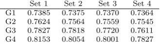
In this section we present several numerical simulations to verify the theoretical estimates provided in Theorem 9 and Theorem 10 in the case of a two dimensional problem on the unit squareΩ= (0,1)2. For the numerical tests, we consider the two sets of meshes shown in Figures 2 and 3. The first set of initial grids are shown in Figure 2 (top line) and consist of 512 (Set 1), 1024 (Set 2), 2048 (Set 3) and 4096 (Set 4) polygonal elements. These meshes have been generated using the software packagePolyMesher[60]. We also consider an initial set of decompositions constisting of 582 (Set 1), 1086 (Set 2), 2198 (Set 3) and 4318 (Set 4) shape-regular triangles as depicted in Figure 3 (top line). Each initial grid is then subsequently coarsened in order to obtain a sequence of nested partitions by employing the software package MGridGen [48, 49].
Set 1 Set 2 Set 3 Set 4
G1
G2
G3
G4
Fig. 2 Sequences of agglomerated grids employed for numerical simulations. Top line: fine grids consisting of 512 (Set 1), 1024 (Set 2), 2048 (Set 3) and 4096 (Set 4) polygonal elements.
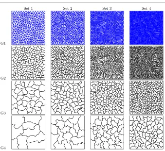
[image:20.595.75.417.70.386.2]Set 1 Set 2 Set 3 Set 4 G1 0.7385 0.7375 0.7370 0.7364 G2 0.7624 0.7564 0.7559 0.7545 G3 0.7827 0.7818 0.7720 0.7611 G4 0.8153 0.8054 0.8001 0.7827
Table 1 Value of the coercivity constantCcoerfor the sets of grids considered in Figure 2 with
Cσj=Cσ= 10,j= 1, . . .,4.
we report the coercivity constantCcoer of (8) for a fixed value of Cσj ≡Cσ = 10 for j = 1, . . . ,4. We observe that the bilinear form is uniformly coercive for a constant value of the penalization coefficient, which is of the same magnitude as the one typically employed on standard shape-regular triangular meshes. As a consequence, in the following, we setCσj ≡Cσ= 10 forj= 1, . . . ,4.
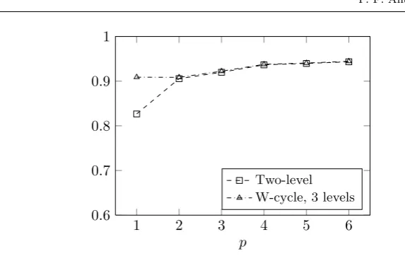
We now consider the sequence of the grids shown in Figure 2, Set 1, and numerically evaluate the constant C2lvlΣJ, J = 2, in Theorem 9 and the con-stantCbΣ3 in Theorem 10, for theh-version of the two solvers, based on selecting
[image:20.595.163.328.427.473.2]in-Set 1 Set 2 Set 3 Set 4
G1
G2
G3
G4
Fig. 3 Sequences of agglomerated grids employed for numerical simulations. Top line: fine grids consisting of 582 (Set 1), 1086 (Set 2), 2198 (Set 3) and 4318 (Set 4) triangular elements.
creases. Notice also that, in practice, the parameterµ = 0, even whenever a p– optimal interpolant cannot be explicetely constructed.
Next, we investigate the performance of the two-level and W-cycle multigrid schemes in terms of the convergence factor
ρ= exp
1 Nln
krNk2
kr0k2
,
whereN denotes the number of iterations required to attain convergence up to a (relative) tolerance of 10−8andr
[image:21.595.77.417.76.387.2]1 2 3 4 5 6 0.6
0.7 0.8 0.9 1
p
Two-level W-cycle, 3 levels
Fig. 4 Estimates ofC2lvlΣJ and bCΣ3 in (24) and (30), respectively, as a function ofp, and
m1=m2=m= 2p2. Sequence of agglomerated meshes shown in Figure 2, Set 1.
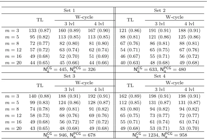
the convergence is faster for larger values of m and the solvers are convergent provided the number of smoothing steps is sufficiently large. For each grid, we have also reported the iteration counts NCGit for the Conjugate Gradient (CG) method, which shows that the two proposed solvers outperform the CG scheme in terms of the number of iterations required to attain convergence, even when a small number of smoothing steps are employed. For the sake of comparison, we also report the iteration countsNPCGit for the Preconditioned Conjugate Gradient (PCG) method, based on employing a simple block Jacobi preconditioner. The extension to polytopic grids of the domain decomposition preconditioning techniques, such as, for example, the ones proposed in [10, 12, 15], in the DG setting, or in [52, 55], in the conforming setting, are currently under investigation and will be the subject of future research. Table 3 presents analogous results for the first three sets of meshes, in the case whenp = 3. Here, we observe that, as expected, the convergence factor increases, but the increase in p does not require an increase in the minimal number of smoothing steps needed to ensure that the underlying multilevel solvers are convergent.
[image:22.595.83.370.72.253.2]Set 1 Set 2
TL W-cycle TL W-cycle
3 lvl 4 lvl 3 lvl 4 lvl
m= 3 133 (0.87) 160 (0.89) 167 (0.90) 121 (0.86) 191 (0.91) 188 (0.91) m= 5 95 (0.82) 113 (0.85) 113 (0.85) 88 (0.81) 121 (0.86) 125 (0.86) m= 8 72 (0.77) 82 (0.80) 81 (0.80) 67 (0.76) 86 (0.81) 88 (0.81) m= 12 57 (0.72) 63 (0.74) 62 (0.74) 54 (0.71) 65 (0.75) 67 (0.76) m= 16 49 (0.68) 52 (0.70) 51 (0.69) 46 (0.67) 55 (0.71) 56 (0.72) m= 20 44 (0.65) 45 (0.66) 44 (0.66) 40 (0.63) 48 (0.68) 49 (0.68)
NCG
it = 445,N PCG
it = 326 N
CG
it = 633,N PCG it = 480
Set 3 Set 4
TL W-cycle TL W-cycle
3 lvl 4 lvl 3 lvl 4 lvl
m= 3 140 (0.88) 188 (0.91) 192 (0.91) 162 (0.89) 198 (0.91) 198 (0.91) m= 5 99 (0.83) 124 (0.86) 128 (0.87) 112 (0.85) 131 (0.87) 131 (0.87) m= 8 74 (0.78) 89 (0.81) 91 (0.82) 83 (0.80) 94 (0.82) 94 (0.82) m= 12 58 (0.73) 68 (0.76) 69 (0.76) 65 (0.75) 73 (0.77) 72 (0.77) m= 16 49 (0.68) 56 (0.72) 57 (0.72) 55 (0.71) 61 (0.74) 61 (0.74) m= 20 43 (0.65) 48 (0.68) 49 (0.68) 49 (0.68) 53 (0.71) 53 (0.70)
NCG
[image:23.595.74.418.78.309.2]it = 946,NPCGit = 678 NCGit = 1234,NPCGit = 958
Table 2 Iteration counts and converge factor (in parenthesis) of the h-version of the two-level and W-cycle solvers and iteration counts of the CG/PCG methods as a function ofm (Cσj≡Cσ= 10,p= 1). Sequences of agglomerated meshes shown in Figure 2.
Set 1 Set 2 Set 3
TL W-cycle TL W-cycle TL W-cycle
3 lvl 4 lvl 3 lvl 4 lvl 3 lvl 4 lvl
m= 3 1281 1334 1342 1168 1272 1362 1230 1379 1391
m= 5 816 832 839 737 790 844 774 852 860
m= 8 546 551 561 487 517 551 513 555 557
m= 12 388 394 400 343 363 385 362 387 384
m= 16 305 312 316 268 284 299 284 301 296
m= 20 254 261 263 222 235 246 235 249 242
NCG
it = 1954,NPCGit = 885 NCGit = 2809,NPCGit = 1264 NCGit = 4174,NPCGit = 1708
Table 3 Iteration counts of theh-version of the two-level and W-cycle solvers as a function ofmand the number of levels and iteration counts of the CG/PCG methods (Cσj≡Cσ= 10, p= 3). Sequences of agglomerated meshes shown in Figure 2.
[image:23.595.73.436.358.468.2]Set 1 Set 2
TL W-cycle TL W-cycle
3 lvl 4 lvl 3 lvl 4 lvl
m= 4 246 (0.90) 258 (0.90) 262 (0.90) 282 (0.89) 291 (0.90) 292 (0.90) m= 6 177 (0.87) 185 (0.87) 188 (0.87) 199 (0.86) 205 (0.87) 204 (0.87) m= 10 120 (0.81) 125 (0.82) 127 (0.82) 133 (0.81) 136 (0.82) 136 (0.82) m= 14 94 (0.77) 98 (0.78) 99 (0.78) 104 (0.77) 106 (0.78) 106 (0.78) m= 18 79 (0.74) 82 (0.74) 83 (0.74) 87 (0.74) 89 (0.75) 89 (0.75)
NCG
it = 551,NPCGit = 369 NCGit = 771,NPCGit = 504
Set 3 Set 4
TL W-cycle TL W-cycle
3 lvl 4 lvl 3 lvl 4 lvl
m= 4 328 (0.90) 333 (0.91) 329 (0.90) 421 (0.91) 425 (0.91) 422 (0.91) m= 6 231 (0.87) 234 (0.88) 232 (0.87) 292 (0.88) 293 (0.89) 292 (0.89) m= 10 153 (0.82) 154 (0.83) 153 (0.82) 190 (0.83) 191 (0.84) 189 (0.84) m= 14 118 (0.78) 119 (0.79) 118 (0.78) 145 (0.79) 148 (0.80) 146 (0.80) m= 18 98 (0.75) 99 (0.75) 98 (0.75) 120 (0.76) 123 (0.77) 122 (0.77)
NCG
[image:24.595.74.413.72.288.2]it = 1145,NPCGit = 718 NCGit = 1630,NPCGit = 974
Table 4 Iteration counts and converge factor (in parenthesis) of theh-version of the two-level and W-cycle solvers and iteration counts of the CG and PCG methods as a function ofm (Cσj≡Cσ= 10,p= 1). Sequences of agglomerated meshes shown in Figure 3.
TL W-cycle NCG
it NPCGit
3 lvl 4 lvl
p= 1 88 121 125 633 480
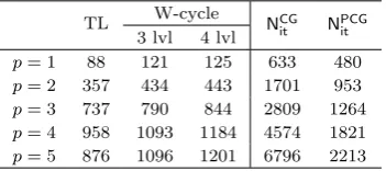
p= 2 357 434 443 1701 953 p= 3 737 790 844 2809 1264 p= 4 958 1093 1184 4574 1821 p= 5 876 1096 1201 6796 2213
Table 5 Iteration counts of theh-version of the two-level and W-cycle solvers as a function ofpand the number of levels and corresponding CG/PCG iteration counts (Cσj ≡Cσ = 10, m= 5). Sequence of agglomerated meshes shown in Figure 2, Set 2.
[image:24.595.158.334.341.419.2]Max. independent set Max. weighted matching Greedy aggregation
ρ N. levels ρ N. levels ρ N. levels NAMG
it
p= 1 0.9990 3 0.9987 7 0.9992 5 >5000
p= 2 0.9989 3 0.9986 8 0.9988 5 >5000
p= 3 0.9989 3 0.9986 8 0.9990 6 >5000
p= 4 0.9989 3 0.9986 9 0.9989 6 >5000
[image:25.595.75.425.82.166.2]p= 5 0.9989 3 0.9986 9 0.9988 6 >5000
Table 6 Number of agglomeration levels (N. levels) and computed convergce factors (ρ) of AlgebraicW-cycle multigrid method (Richardon smoother,m= 5 pre- and post-smoothing steps) as a function ofp. The agglomerates are formed algebraically by using either the maximal independent set, the (approximate) maximum weighted matching or the greedy aggregation algorithms. The initial fine grid is shown in Figure 2, Set 2 (first row).
account in the construction of the solver and/or more sophisticated (aggressive) aggregation-based algebraic algorithms, as well as Schwarz-type smoothers, such as the ones proposed, for example, in [51, 24], should be considered. Such develop-ments are currently under investigation and will be the subject of future research.
7 Conclusions
We have presented and analyzed two-level and multigrid schemes for the efficient solution of the linear system of equations arising from thehp-version of the inte-rior penalty DG scheme on polygonal/polyhedral meshes. The attractive feature of the proposed algorithms is that the auxiliary sequence of meshes needed by the multilevel solver can be generated by a (successive) general geometric agglomera-tion procedure starting from an initial grid made of (possibly arbitrarily-shaped) elements. Such an approach fully exploits the flexibilty of DG methods in terms of their ability to handle arbitrarily-shaped elements, including polytopic elements, see [4, 8, 36, 21, 35, 6, 33], and the recent review paper [5]. Extending the theoretical results recently presented in [13] on quasi-uniform meshes, we have proved that, under mild geometric assumptions on the quality of the agglomerates, both the two-level and W-cycle multigrid schemes converge uniformly with respect to the discretization parameters (namely, the granularity of the underlying partition and the polynomial approximation degreep) and, for the multigrid scheme, the num-ber of levels, provided that the numnum-ber of smoothing steps is chosen sufficiently large. We have also demonstrated through numerical experiments that the theo-retical assumption concerning the need to employ a sufficiently large number of smoothing steps is not needed in practice, i.e., our algorithms converge even if the number of smoothing steps is kept fixed independently of the polynomial approx-imation degree p. However, in this latter case, the performance of the iterative solvers deteriorates, as expected, when increasingp.
References
2. P. F. Antonietti, L. Beir˜ao Da Veiga, S. Scacchi, and M. Verani. A C1 virtual element method for the Cahn-Hilliard equation with polygonal meshes. SIAM J. Numer. Anal., 54(1):34–56, 2016.
3. P. F. Antonietti, F. Brezzi, and L. Marini. Stabilizations of the Baumann-Oden DG formulation: the 3D case.Boll. Unione Mat. Ital. (9), 1(3):629–643, 2008.
4. P. F. Antonietti, F. Brezzi, and L. D. Marini. Bubble stabilization of discontinuous Galerkin methods. Comput. Methods Appl. Mech. Engrg., 198(21-26):1651–1659, 2009. 5. P. F. Antonietti, A. Cangiani, J. Collis, Z. Dong, E. H. Georgoulis, S. Giani, and P.
Hous-ton. Review of Discontinuous Galerkin finite element methods for partial differential equa-tions on complicated domains. G.R. Barrenechea et al. (eds.), Building Bridges: Connec-tions and Challenges in Modern Approaches to Numerical Partial Differential EquaConnec-tions,
Lecture Notes in Computational Science and Engineering114:279–307, 2016.
6. P. F. Antonietti, C. Facciola, A. Russo, and M. Verani. Discontinuous Galerkin approx-imation of flows in fractured porous media on polygonal and polyhedral meshes. MOX Report 55/2016, 2016.
7. P. F. Antonietti, L. Formaggia, A. Scotti, M. Verani, and V. Nicola. Mimetic finite dif-ference approximation of flows in fractured porous media. M2AN Math. Model. Numer. Anal., 50(3):809–832, 2016.
8. P. F. Antonietti, S. Giani, and P. Houston. hp–Version composite discontinuous Galerkin methods for elliptic problems on complicated domains. SIAM J. Sci. Comput., 35(3):A1417–A1439, 2013.
9. P. F. Antonietti, S. Giani, and P. Houston. Domain decomposition preconditioners for Discontinuous Galerkin methods for elliptic problems on complicated domains. J. Sci. Comput., 60(1):203–227, 2014.
10. P. F. Antonietti and P. Houston. A class of domain decomposition preconditioners for hp-discontinuous Galerkin finite element methods. J. Sci. Comput., 46(1):124–149, 2011. 11. P. F. Antonietti and P. Houston. Preconditioning high-order discontinuous Galerkin dis-cretizations of elliptic problems.Lecture Notes in Computational Science and Engineering, 91:231–238, 2013.
12. P. F. Antonietti, P. Houston, and I. Smears. A note on optimal spectral bounds for nonoverlapping domain decomposition preconditioners for hp-version discontinuous Galerkin methods. Int. J. Numer. Anal. Model., 13(4):513–524, 2016.
13. P. F. Antonietti, M. Sarti, and M. Verani. Multigrid algorithms for hp-discontinuous Galerkin discretizations of elliptic problems.SIAM J. Numer. Anal., 53(1):598–618, 2015. 14. P. F. Antonietti, M. Sarti, and M. Verani. Multigrid algorithms for high order discon-tinuous Galerkin methods. Lecture Notes in Computational Science and Engineering, 104:3–13, 2016.
15. P. F. Antonietti, M. Sarti, M. Verani, and L. T. Zikatanov. A uniform additive Schwarz preconditioner for high-order discontinuous Galerkin approximations of elliptic problems.
J. Sci. Comput., 70(2):608–630, 2017.
16. D. N. Arnold. An interior penalty finite element method with discontinuous elements.
SIAM J. Numer. Anal., 19(4):742–760, 1982.
17. D. N. Arnold, F. Brezzi, B. Cockburn, and L. D. Marini. Unified analysis of discontin-uous Galerkin methods for elliptic problems. SIAM J. Numer. Anal., 39(5):1749–1779, 2001/2002.
18. J. Aubin. Approximation des probl`emes aux limites non homog`enes pour des op´erateurs non lin´eaires. J. Math. Anal. Appl., 30:510–521, 1970.
19. I. Babuˇska. The finite element method with penalty.Math. Comp., 27(122):221–228, 1973. 20. G. A. Baker. Finite element methods for elliptic equations using nonconforming elements.
Math. Comp., 31(137):45–59, 1977.
21. F. Bassi, L. Botti, A. Colombo, F. Brezzi, and G. Manzini. Agglomeration-based physical frame dg discretizations: An attempt to be mesh free. Math. Models Methods Appl. Sci., 24(8):1495–1539, 2014.
22. F. Bassi, L. Botti, A. Colombo, D. A. Di Pietro, and P. Tesini. On the flexibility of agglomeration based physical space discontinuous Galerkin discretizations. J. Comput. Phys., 231(1):45–65, 2012.
25. L. Beir˜ao Da Veiga, F. Brezzi, A. Cangiani, G. Manzini, L. D. Marini, and A. Russo. Basic principles of virtual element methods.Math. Models Methods Appl. Sci., 23(01):199–214, 2013.
26. L. Beir˜ao Da Veiga, F. Brezzi, L. Marini, and A. Russo. Mixed virtual element methods for general second order elliptic problems on polygonal meshes.M2AN Math. Model. Numer. Anal., 50(3):727–747, 2016.
27. L. Beir˜ao Da Veiga, F. Brezzi, L. Marini, and A. Russo. Virtual element method for general second-order elliptic problems on polygonal meshes.Math. Models Methods Appl. Sci., 26(4):729–750, 2016.
28. L. Beir˜ao da Veiga, K. Lipnikov, and G. Manzini.The mimetic finite difference method for elliptic problems, volume 11 ofMS&A. Modeling, Simulation and Applications. Springer, Cham, 2014.
29. J. Bramble. Multigrid Methods. Number 294 in Pitman Research Notes in Mathematics Series. Longman Scientific & Technical, Harlow, UK, 1993.
30. F. Brezzi, K. Lipnikov, and M. Shashkov. Convergence of the mimetic finite difference method for diffusion problems on polyhedral meshes.SIAM J. Numer. Anal., 43(5):1872– 1896 (electronic), 2005.
31. F. Brezzi, K. Lipnikov, and M. Shashkov. Convergence of mimetic finite difference method for diffusion problems on polyhedral meshes with curved faces. Math. Models Methods Appl. Sci., 16(2):275–297, 2006.
32. F. Brezzi, K. Lipnikov, and V. Simoncini. A family of mimetic finite difference methods on polygonal and polyhedral meshes. Math. Models Methods Appl. Sci., 15(10):1533–1551, 2005.
33. A. Cangiani, Z. Dong, and E. Georgoulis. hp-Version space-time discontinuous Galerkin methods for parabolic problems on prismatic meshes. Submitted for publication, 2016. 34. A. Cangiani, Z. Dong, E. Georgoulis, and P. Houston.hp–Version discontinuous Galerkin
methods on polygonal and polyhedral meshes. 2016, in preparation.
35. A. Cangiani, Z. Dong, E. Georgoulis, and P. Houston. hp-Version discontinuous Galerkin methods for advection-diffusion-reaction problems on polytopic meshes. M2AN Math. Model. Numer. Anal., 50(3):699–725, 2016.
36. A. Cangiani, E. H. Georgoulis, and P. Houston.hp-Version discontinuous Galerkin meth-ods on polygonal and polyhedral meshes.Math. Models Methods Appl. Sci., 24(10):2009– 2041, 2014.
37. T. F. Chan, J. Xu, and L. Zikatanov. An agglomeration multigrid method for unstruc-tured grids. InDomain decomposition methods, 10 (Boulder, CO, 1997), volume 218 of
Contemp. Math., pages 67–81. Amer. Math. Soc., Providence, RI, 1998.
38. B. Cockburn, G. E. Karniadakis, and C.-W. Shu, editors.Discontinuous Galerkin methods, Springer-Verlag, Berlin, 2000. Theory, computation and applications. Papers from the 1st International Symposium held in Newport, RI, May 24-26, 1999.
39. D. A. Di Pietro and A. Ern. Mathematical aspects of discontinuous Galerkin meth-ods, volume 69 ofMath´ematiques & Applications (Berlin) [Mathematics & Applications]. Springer, Heidelberg, 2012.
40. T.-P. Fries and T. Belytschko. The extended/generalized finite element method: An overview of the method and its applications. Internat. J. Numer. Methods Engrg., 84(3):253–304, 2010.
41. E. H. Georgoulis. Inverse-type estimates on hp-finite element spaces and applications.
Math. Comp., 77(261):201–219 (electronic), 2008.
42. W. Hackbusch.Multi-grid methods and applications, volume 4 ofSpringer series in com-putational mathematics. Springer, Berlin, 1985.
43. W. Hackbusch and S. Sauter. Composite finite elements for problems containing small geometric details. Part II: Implementation and numerical results. Comput. Visual Sci., 1(4):15–25, 1997.
44. W. Hackbusch and S. Sauter. Composite finite elements for the approximation of PDEs on domains with complicated micro-structures. Numer. Math., 75(4):447–472, 1997. 45. J. S. Hesthaven and T. Warburton. Nodal Discontinuous Galerkin Methods: Algorithms,
48. I. Moulitsas and G. Karypis. Mgridgen/Parmgridgen Serial/Parallel Library for Generating Coarse Grids for Multigrid Methods. University of Minnesota, De-partment of Computer Science/Army HPC Research Center, 2001. Available at: www-users.cs.umn.edu/~moulitsa/software.html.
49. I. Moulitsas and G. Karypis. Multilevel algorithms for generating coarse grids for multigrid methods,. InSupercomputing 2001 Conference Proceedings, 2001.
50. J. Nitsche. ¨Uber ein Variationsprinzip zur L¨osung von Dirichlet Problemen bei Verwen-dung von Teilr¨aumen, die keinen Randbedingungen unterworfen sind. Abh. Math. Sem. Uni. Hamburg, 36:9–15, 1971.
51. L. N. Olson and J. B. Schroder. Smoothed aggregation multigrid solvers for high-order discontinuous Galerkin methods for elliptic problems. J. Comput. Phys., 230(18):6959– 6976, 2011.
52. L. F. Pavarino. Additive Schwarz methods for thep-version finite element method.Numer. Math., 66(4):493–515, 1994.
53. W. Reed and T. Hill. Triangular mesh methods for the neutron transport equation. Technical Report LA-UR-73-479, Los Alamos Scientific Laboratory, 1973.
54. B. Rivi`ere. Discontinuous Galerkin methods for solving elliptic and parabolic equations, volume 35 ofFrontiers in Applied Mathematics. Society for Industrial and Applied Math-ematics (SIAM), Philadelphia, PA, 2008. Theory and implementation.
55. J. Sch¨oberl, J. M. Melenk, C. Pechstein, and S. Zaglmayr. Additive Schwarz precondi-tioning forp-version triangular and tetrahedral finite elements. IMA J. Numer. Anal., 28(1):1–24, 2008.
56. C. Schwab. p- and hp-finite element methods. Numerical Mathematics and Scientific Computation. The Clarendon Press, Oxford University Press, New York, 1998. Theory and applications in solid and fluid mechanics.
57. E. Stein. Singular Integrals and Differentiability Properties of Functions. Princeton, University Press, Princeton, N.J., 1970.
58. N. Sukumar and A. Tabarraei. Conforming polygonal finite elements.Internat. J. Numer. Methods Engrg., 61(12):2045–2066, 2004.
59. A. Tabarraei and N. Sukumar. Extended finite element method on polygonal and quadtree meshes. Comput. Methods Appl. Mech. Engrg., 197(5):425–438, 2008.
60. C. Talischi, G. Paulino, A. Pereira, and I. Menezes. Polymesher: A general-purpose mesh generator for polygonal elements written in Matlab. Structural and Multidisciplinary Optimization, 45(3):309–328, 2012.