ISSN Online: 2327-4379 ISSN Print: 2327-4352
DOI: 10.4236/jamp.2020.81006 Jan. 6, 2020 70 Journal of Applied Mathematics and Physics
Bayesian Regularized Quantile Regression
Analysis Based on Asymmetric Laplace
Distribution
Qiaoqiao Tang, Haomin Zhang
*, Shifeng Gong
School of Science, Guilin University of Technology, Guilin, China
Abstract
In recent years, variable selection based on penalty likelihood methods has aroused great concern. Based on the Gibbs sampling algorithm of asymmetric Laplace distribution, this paper considers the quantile regression with adap-tive Lasso and Lasso penalty from a Bayesian point of view. Under the non- Bayesian and Bayesian framework, several regularization quantile regression methods are systematically compared for error terms with different distribu-tions and heteroscedasticity. Under the error term of asymmetric Laplace dis-tribution, statistical simulation results show that the Bayesian regularized quantile regression is superior to other distributions in all quantiles. And based on the asymmetric Laplace distribution, the Bayesian regularized quan-tile regression approach performs better than the non-Bayesian approach in parameter estimation and prediction. Through real data analyses, we also con-firm the above conclusions.
Keywords
Asymmetric Laplace Distribution, Gibbs Sampling, Adaptive Lasso, Lasso, Bayesian Regularization Quantile Regression
1. Introduction
Since the pioneering work by Koenker and Bassett in 1978, quantile regression (QR) has been deeply studied and widely applied to descript the elaborate rela-tionship between the dependent variable and predictors [1]. Compared with the traditional mean regression, quantile regression has more robustness to data with outliers. In 1999, Koenker and Machado connected the asymmetric Laplace distribution (ALD) to QR model and defined a goodness-of-fit criterion for
quan-How to cite this paper: Tang, Q.Q., Zhang, H.M. and Gong, S.F. (2020) Bayesian Re-gularized Quantile Regression Analysis Based
on Asymmetric Laplace Distribution.
Jour-nal of Applied Mathematics and Physics, 8, 70-84.
https://doi.org/10.4236/jamp.2020.81006 Received: December 4, 2019
Accepted: January 3, 2020 Published: January 6, 2020
Copyright © 2020 by author(s) and Scientific Research Publishing Inc. This work is licensed under the Creative Commons Attribution International License (CC BY 4.0).
http://creativecommons.org/licenses/by/4.0/
DOI: 10.4236/jamp.2020.81006 71 Journal of Applied Mathematics and Physics tile regression, which is the natural analog of R2 statistic of least squares regres-sion [2]. In 2001, Yu and Moyeed first proposed a Bayesian quantile regression model that the error follows an asymmetric Laplace ( AL) distribution, and proved the maximization of likelihood-based inference used independently dis-tributed asymmetric Laplace densities was equivalent to the minimization of the loss function [3]. In 2010, Hewson and Yu suggested quantile regression model for binary data within the Bayesian framework [4]. In 2011, Reich et al. intro-duced Bayesian spatial quantile regression model [5]. In 2013, Sriram et al. showed that the misspecified likelihood in the ALD approach still leads to con-sistent results [6]. In 2009, Kozumi and Kobayashi built a more efficient Gibbs sampler for fitted the quantile regression model based on a location-scale mix-ture of the asymmetric Laplace distribution to draw samples from the posterior distribution [7]. In 2012, Khare and Hobert proved that this new sampling algo-rithm converges at a geometric rate [8]. In 2015, Sriram proposed a correction to the MCMC iterations to construct asymptotically valid intervals [9].
In 2004, Koenker added the Lasso regularization method to the mixed-effect quantile regression model for the first time, and the Lasso penalty made the random effect shrink to zero [10]. In 2007, Wang et al. considered the least absolute deviance (LAD) estimate with adaptive Lasso penalty (LAD-lasso) and proved its oracle property [11]. In 2008, Li and Zhu considered quantile regression with the Lasso penalty and developed its piecewise linear solution path [12]. In 2009, Wu and Liu studied the quantile regression with the SCAD method and the adaptive Lasso method [13]. In 2008, Park and Casella studied the Lasso penalty from the Bayesian angle, and proposed that the hierarchical model can be effectively solved by the Gibbs sampler, thereby introducing the regularization method [14]. In 2010, Li et al. studied the regularization method in quantile regression from the perspective of Bayesian and proposed to set the prior distribution of parameters to Laplace prior, and use Gibbs sampler to sampling Bayesian Lasso quantile regression [15]. In 2012, Alhamzawi et al. proposed Bayesian adaptive Lasso quantile regression, by setting different pe-nalty parameters for different variables, and setting the pepe-nalty parameter to in-verse gamma distribution, and the inin-verse gamma priori Parameters are treated as unknowns and estimated along with other parameters [16]. In 2018, Adlouni
et al. showed that a regularized quantile regression model with B-Splines based
on five penalties (Lasso, Ridge, SCAD0, SCAD1 and SCAD2) in Bayesian frame-work [17].
DOI: 10.4236/jamp.2020.81006 72 Journal of Applied Mathematics and Physics
2. Methods
2.1. Quantile Regression
Given data
{
(
x y ii, i)
, 1, ,= n}
, with covariate vector xi′ =(
x xi1, , ,i2 xik)
and(
y1, ,yn)
′ =
y is the response variable. The θth quantile regression model
for the response yi given xi takes the form of
(
)
( )
,i
y i i
Q
θ
x =x′β
θ
(1)where
(
)
F 1(
)
i i
y i y i
Q
θ
x = −θ
x is the inverse cumulative distribution function and( )
θβ is the unknown coefficients vector that is dependent on the quantile θ,
( )
0,1θ∈ .
The regression parameter
β
can be estimated by minimizating the following objective function(
)
1
min n i i ,
i θ
β
∑
= ρ y x− ′β (2) whereρ
θ( )
u =u(
θ
−I(
u<0)
)
is the loss function and I( )
⋅ denotes the indi-cator function.In 2001, Yu and Moyeed [3] argued that the minimization problem in equa-tion (2) is equivalent to maximizing the likelihood funcequa-tion of yi by
assum-ing yi’s are random variables from a skewed Laplace distribution with i
µ=x′β and σ =1. The density function of a skewed Laplace distribution is given by
(
, ,)
(
1)
exp(
y)
,f y µ σ θ θ θ ρθ µ
σ σ
− −
= −
(3)
where, σ is the scale parameter, µ is the location parameter and θ is the asymmetrc parameter.
Then the likelihood function of the sample y=
(
y y1, , ,2 yn)
′ can beex-pressed as
(
)
(
)
(
)
1
1 1
L , , exp .
n n n i n i y θ θ θ
µ σ θ ρ µ
σ
σ =
−
= − −
∑
y (4)
Tsionas [18], Kozumi and Kobayashi [7] have demonstrated that ALD can be viewed as a mixture of standard an exponential distribution, exp 1
( )
and a standard normal distribution N 0,1( )
. Assume that z and υ represent a stan-dard exponential distribution and a stanstan-dard normal distribution, respectively. For 1 2(
)
1 θ ω θ θ − = − ,
(
)
2 1 fθ
θ
=− , if µ∼ALD
(
0, ,σ θ)
, random variable1 2
z z
µ ω= +φσ− υ, Therefore, it can be known that the independent variable
i
y of the quantile regression is equivalent to 1
2 .
i iβ ωzi φσ zi iυ −
′
= + +
DOI: 10.4236/jamp.2020.81006 73 Journal of Applied Mathematics and Physics
2.2. Bayesian Quantile Regression with Lasso and Adaptive Lasso
Penalty
The Bayesian quantile regression parameter estimation model with Lasso penalty (Li and Zhu) [12] is
(
)
1
min n i i k j ,
i θ j
β
∑
ρ y x− ′β +λ∑
= β (6)Li et al. [15] set the prior distribution of the parameter βj to a Laplace prior
(
)
(
)
1
| , 2 expk k
j j
j
p β σ λ σλ σλ β
=
= −
∑
. It is also assumed that the error termi
µ obeys the asymmetric Laplace distribution (ALD).
Bayesian quantile regression with adaptive Lasso penalty (BQR-AL) is based on different penalty parameters are applied to different regression coefficients. Therefore, the parameter estimation model of BQR-AL is
(
)
1 1
min n i i k j j ,
i θ j
β
∑
= ρ y x− ′β +∑
= λ β (7) Alhamzawi and Yu [16] proposed different penalization parameters for dif-ferent regression coefficients, and the prior of the penalty parameters is set to the inverse gamma distribution, and treat the hyperparameters of the inverse gam-ma prior as unknowns. Thus, the Laplace prior on βj by(
)
1 1
2 2
| , exp ,
2
j
j j
j j
p β σ λ σ σ β
λ λ = − (8)
Andrews and Mallows [19] mentioned that
{
}
0 1 2 2 2exp exp exp d , 0.
2 2 2 2 2
t
t s s
s s
ξ ξ ∞ ξ ξ ξ
− = − − >
π
∫
(9)Let 1 2 j σ η λ
= , (8) can be written as
(
| ,)
exp{
}
,2
j j j
p β σ λ =η −η β (10)
also equivalent to
(
)
{
2}
2{
2}
0 1
| , exp 2 exp 2 d ,
2 2
j j j j j j
j
p s s s
s
η
β σ λ
= ∞ −β
−η
π
∫
(11)so there are
(
2)
{
2}
{
2}
2 0
1
| , exp 2 exp 2 d .
2 2
j j j j j j j
j j
p s s s
s
σ
β σ λ β σ λ
λ ∞
= − −
π
∫
(12)The prior distribution of 2
j
distri-DOI: 10.4236/jamp.2020.81006 74 Journal of Applied Mathematics and Physics bution density function of 2
j
λ
is(
2)
( )
( )
2 12
| , exp ,
j j
j
p λ δ γ γδ λ δ γ
δ λ
− −
= −
Γ
(13)
where δ >0 and
γ
>0 are two hyperparameters. Yi and Xu [20] pointed out that the values of these two hyperparameters determine the degree of compres-sion of the variables in (13), because small γ large δ will lead to greater compression, so in order to avoid the impact of special values on the estimation of regression coefficients, we consider δ and γ as unknown parameters.In summary, the Bayesian quantile regression hierarchical model with adap-tive Lasso penalty is
( )
( )
(
)
{
}
1 2 0 2 , 1,1 exp ,
2 2
| exp ,
i i i i i
i i i i z z p p
p z z
β ω φσ υ
β
υ υ
σ σ σ
− ′ = + + ∝ = −
π
= − y x
(
)
{
}
{
}
(
)
( )
( )
( )
{
}
(
)
2 2 2
2 1 2 2 2 1 1 1
, | , exp 2 exp 2 ,
2 2
| , exp ,
exp ,
, .
j j j j j j j
j j
j j
j a
p s s s
s p p b p δ δ σ
β σ λ β σ λ
λ
τ γ
λ δ γ λ
δ λ
σ σ σ
γ δ γ
− − − − = − − π = −
Γ
= −
=
(14)
2.3. Gibbs Sampling
From the hierarchical model, the joint posterior density function of each para-meter is
(
)
(
)
(
)
(
) (
)
( ) (
)
(
)
{
}
{
}
( )
( )
1 2 2 1 1 2 2 1 2 1 2 2 2 1 12 1 1
2
, , , , , , | ,
| , , , | , | , | , ,
exp
2
1 exp 2 exp 2
2 2
exp exp
k
n k
i j j j j
i j
n
i i i
i
i i i
k
j j j j
j j j
a j
j
p
p p z p s p p p
ωz z z z s s s δ δ
σ λ λ
σ σ β σ λ λ γ δ σ γ δ
σ
σ σ
φ σ φ
σ
β σ λ
λ
γ λ γ γ σ
δ λ = = − = = − − − − ∝ − ′ − ∝ − − × − − π × − −
Γ
∏
∏
∏
∏
z s y Χ
y z Χ
y x
β
β
β
{
bσ}
,where
(
y y1, , ,2 yn)
,(
x x1, , ,2 xn)
,(
z z1, , ,2 zn)
,(
s s1, , ,2 sk)
.= = = =
y Χ z s
DOI: 10.4236/jamp.2020.81006 75 Journal of Applied Mathematics and Physics
(
)
(
0)
2 0 0 2 2 2 2
| N , ,
| N , ,
1
| GIG , , ,
2 1
| GIG , , ,
2 2 j j j i j j j z s β β β β β β α σ β λ ⋅ ⋅ ⋅ ⋅ s s ∼ ∼ ∼ ∼
(
)
31 2
2
2
1
| G , ,
| GIG 1 , ,
2
| G 1, .
j j k j j a a s k σ σ
λ δ γ
γ δ λ−
= ⋅ ⋅ + + ⋅ −
∑
∼ ∼ ∼ (15) Here(
)
(
)
2 2 2 2 1 22 2 2
1 1 2 , , 3 , 2 . 2 i i
n k j
i i i
i
i i j j
a n k a
s z
a z b
z
α σω φ σ σφ ω φ λ − − = = = + ′ = − = + + − ′ − = + + +
∑
∑
y x y x β β(16)
Since the full condition posterior distribution
( )
(
( )
)
2 1| k k k
j j
p δ δ − γ δ λ−δ
=
⋅ ∝ Γ
∏
of δ does not have a closed form, it is a logarithmic convex function. Gilks [21] proposed using the adaptive rejection sampling algorithm to sample this distribution.
3. Simulation Studies
Based on the MCMC algorithm of Gibbs sampling, Bayesian estimation is carried out on the model. The simulation studies used to compare the regula-rized quantile regression under the Bayesian and the non-Bayesian frame-work. These methods include Bayesian quantile regression with adaptive Lasso penalty (BQR-AL), Bayesian quantile regression with Lasso penalty (BQR-L), quantile regression with Lasso penalty (QR-L), quantile regression with SCAD penalty (QR-SCAD) and quantile regression (QR).
3.1. Independent and Identically Distributed Random Errors
Here, we follow the same simulation strategy introduced by Li, Xi and Lin [15]in the simulation studies 1, 2 and 3 with different parameter values for the error distributions.
We consider a linear model
, 1, ,
i= i′ +εi i= n
DOI: 10.4236/jamp.2020.81006 76 Journal of Applied Mathematics and Physics where εi’s have the θth quantile equal to zero.
For i.i.d. random errors, this paper will consider the following four forms of
simulation
Simulation 1: β=
(
3,1.5,0,0,2,0,0,0)
,Simulation 2: β =
(
0.85,0.85,0.85,0.85,0.85,0.85,0.85,0.85)
,Simulation 3: β =
(
5,0,0,0,0,0,0,0)
,Simulation 4:
10 10 10
3, ,3,0, ,0,3, ,3
β=
.
In the first three simulation studies, the rows of x is generated in a multiva-riate normal distribution N 0,
( )
Σ with( )
0.5i jij
−
Σ = . In Simulation 4, we first generate Ζ1 and Ζ2 from N 0,1
( )
, then let xj =Ζ ν1+ j, j=1, ,10 ,( )
N 0,1
j
x ∼ , j=11, ,20 , xj =Ζ2+νj, where j=21, ,30 , where
(
)
N 0,0.01
j
ν ∼ , j=1, ,10,21, ,30 .
In each simulation, we consider the error distributions in our simulation fol-lows
1) A normal distribution N ,1
( )
µ with the θth quantile equal to zero. 2) A Laplace distribution Laplace( )
µ,1 with the θth quantile equal to zero.3) A t distribution with three degrees of freedom, t( )3 . 4) A χ2 distribution with three degrees of freedom,
( )23
χ
.5) A asymmetric Laplace distribution ALD
(
µ,0.5,1)
with the θth quantile equal to zero.The number of observations in one simulated sample is n = 200. The simula-tion is repeated 50 times for each error distribusimula-tion. The evaluasimula-tion index is the median mean absolute deviation (MMAD), i.e.
200 1
ˆ
MMAD median 1 200 true
i i
i=
′ ′
= −
∑
xβ xβ The quantile regression model for the quantile θ=
(
0.3,0.5,0.7)
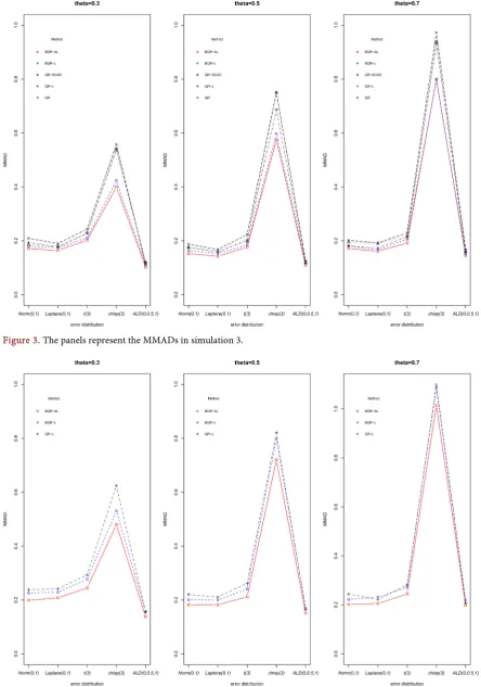
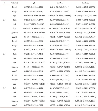
is estimatedseparately. The simulation results are shown in Figures 1-4.
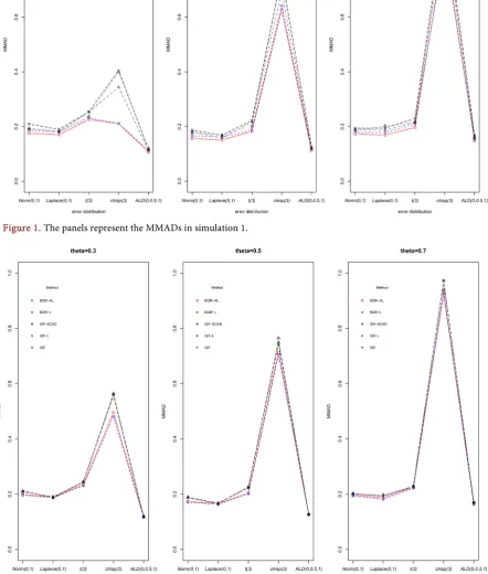
Figure 1 shows that under the condition of simulation 1, that is, sparse coeffi-cients, the MMD values of BQR-AL and BQR-L are lower than those of the fre-quency school method, in which the MMAD value satisfying the error term compliance distribution ALD
(
µ,0.5,1)
is smaller.Figure 2 corresponds to the dense coefficient in simulation 2, and it can be seen that the MMAD values of BQR-AL and BQR-L are very small and close to each other.
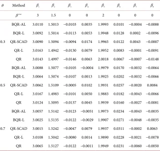
Figure 3 corresponds to the case where the coefficient of the simulation 3 is sparse, and the same conclusion as the simulation 1 can still be obtained. And the effect of Bayesian regularized quantile regression is more obvious.
DOI: 10.4236/jamp.2020.81006 77 Journal of Applied Mathematics and Physics
Figure 1. The panels represent the MMADs in simulation 1.
[image:8.595.96.539.178.699.2]DOI: 10.4236/jamp.2020.81006 78 Journal of Applied Mathematics and Physics
[image:9.595.100.541.386.704.2]Figure 3. The panels represent the MMADs in simulation 3.
DOI: 10.4236/jamp.2020.81006 79 Journal of Applied Mathematics and Physics
Figures 1-4 show that, in terms of the MMAD, BQR-AL and BQR-L method performs better than the other regularized quantile regression method. The re-sults of the MMAD for simulation 1 - 4 are reported in Figures 1-4. From these simulation, we can learn the following results:
1) In the above simulation, the MMADs of BQR-AL and BQR-L tend to give lower MMAD compared with the other regularized quantile regression under non-Bayesian for all distributions under considerations. It is shown that the sta-bility and repeatasta-bility of the Bayesian regularized quantile regression are better. 2) In the case of sparse and very sparse regression coefficient, the MMAD value of BQR-AL is the smallest. In the case of dense regression coefficient, the MMAD value of BQR-L is smaller. Moreover, the estimation effect of the two methods is similar.
3) The BQR-AL and BQR-L methods can achieve good results under all error term distributions. It is shown that the regularized Bayesian quantile regression method is robust to the assumption of the error term, and the two methods are satisfactory even if the error term deviates from ALD.
4) No matter what the distribution of the original data is, when the error dis-tribution is ALD, the regularized quantile regression method under Bayesian framework has high accuracy, especially the BQR-AL method, and the estimated value of its parameters is the closest to the real value.
In addition to observing the MMADs of each method, this paper can also ob-serve the estimation of its parameters. Due to the limited space, in this paper, the parameter estimation results of error obeying ALD distribution in simulation 1 are simulated:
It can be seen from the parameter estimates in Table 1, the QR class method generally gives less biased parameter estimates, but this does not guarantee a good quantile prediction, as implied by the MMADs in Figure 4.
3.2. Non-
i.i.d.
Random Errors
Consider the following model when the error term is subject to a non-i.i.d.
(
)
1 2 3 3
2 1 ,
y= + +x x +x + +x ε
where x1∼N 0,1
( )
, x U3 ∼( )
0,1 , x2∼x x1+ 3+z, where z∼N 0,1( )
and( )
N 0,1
ε∼ . The remaining five noise variables x x x x x4, , , ,5 6 7 8 are generated from the independent standard normal distribution. The results are shown in
Table 2 and are based on 50 repetitions, each with sample size n = 200.
It can be known from Table 2 that the BQR-L method have smaller MMAD values, indicating that the regularized quantile regression method under the Bayesian framework is also superior to the regularized quantile regression me-thod under the non-Bayesian framework when the error obeys the non-i.i.d..
3.3. Prostate Cancer Data Set
This section mainly analyzes prostate cancer data in the “bayesQR” package
DOI: 10.4236/jamp.2020.81006 80 Journal of Applied Mathematics and Physics
Table 1. Parameter estimates for simulation 1 in the case of i.i.d.
θ Method β1 β2 β3 β4 β5 β6 β7 β8
true
β 3 1.5 0 0 2 0 0 0
0.3
BQR-AL 3.0110 1.5013 −0.0103 0.0035 1.9993 0.0101 −0.0004 −0.0088
BQR-L 3.0092 1.5014 −0.0113 0.0053 1.9948 0.0128 0.0002 −0.0096
QR-SCAD 3.0090 1.5094 −0.0094 0.0174 1.9965 0.0122 0.0043 −0.0007
QR-L 3.0163 1.4942 −0.0130 0.0079 1.9952 0.0083 −0.0001 −0.0091
QR 3.0143 1.4997 −0.0146 0.0063 2.0018 0.0067 −0.0007 −0.0148
0.5
BQR-AL 3.0088 1.5077 −0.0105 −0.0004 1.9979 0.0170 −0.0032 −0.0064
BQR-L 3.0064 1.5074 −0.0107 0.0013 1.9925 0.0202 −0.0032 −0.0066
QR-SCAD 3.0062 1.5109 −0.0005 0.0102 1.9931 0.0257 −0.0020 0.0084
QR-L 3.0167 1.4983 −0.0101 0.0050 1.9883 0.0182 −0.0043 −0.0066
QR 3.0124 1.5095 −0.0137 0.0045 1.9939 0.0160 −0.0027 −0.0081
0.7
BQR-AL 3.0057 1.5142 −0.0123 −0.0051 1.9973 0.0234 −0.0043 −0.0035
BQR-L 3.0025 1.5135 −0.0122 −0.0029 1.9907 0.0271 −0.0048 −0.0035
QR-SCAD 3.0015 1.5242 −0.0047 0.0079 1.9937 0.0311 −0.0002 0.0063
QR-L 3.0108 1.5042 −0.0080 0.0014 1.9890 0.0228 −0.0021 −0.0078
QR 3.0065 1.5127 −0.0122 −0.0011 1.9949 0.0231 −0.0060 −0.0050
Table 2. MMADs of each method in the case of non-i.i.d.
θ 0.3 0.5 0.7
BQR-AL 0.67640 1.58100 2.44680
BQR-L 0.65308 1.55980 2.41390
QR-SCAD 0.72930 1.57730 2.43000
QR-L 0.69427 1.57320 2.43920
QR 0.72090 1.59810 2.48700
record of 97 male patients undergoing radical prostatectomy, containing the lev-el of prostate antigen y (lpsa) and eight influencing factors. These influencing factors were: log cancer volume (lcavol), log prostate weight (lweight), age, log of the amount of benign prostatic hyperplasia (lbph), seminal vesicle invasion (svi), log of capsular penetration (lcp), Gleason score (gleason) and percentage of Gleason score 4 or 5 (pgg 45). As with the numerical simulation of the second part, still consider θ=
(
0.3,0.5,0.7)
here. [image:11.595.207.539.424.527.2]DOI: 10.4236/jamp.2020.81006 81 Journal of Applied Mathematics and Physics first 1000 samples are discarded. The results are shown in Table 3.
It can be seen from Table 3 that the parameter estimates of the BQR-L and BQR-AL methods are very close to the classical quantile regression and the credible intervals of the BQR-L and BQR-AL methods are narrower than the QR, in which the BQR-AL interval to be more accurate than BQR-L, from this point of view, the Bayesian quantile regression method with penalty is estimated to be more accurate than the non-Bayesian regularized quantile regression me-thod.
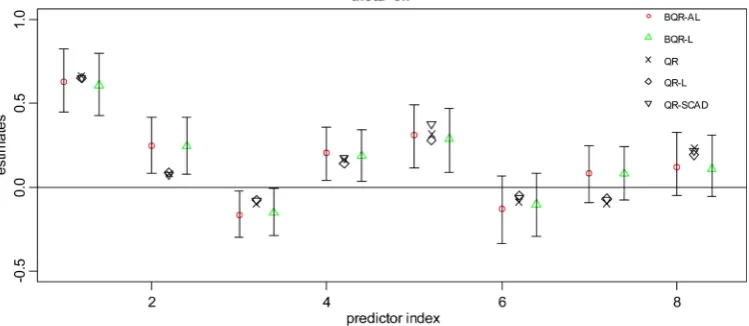
[image:12.595.149.538.294.737.2]Of course, we can also intuitively understand by drawing images. In this sec-tion, for a more intuitive observasec-tion, the estimated values of the various me-thods for θ =0.7 are plotted, and similar results are obtained for other quan-tiles. In order to be intuitive, the estimated values of each method will be trans-lated, and the image is drawn as shown in Figure 5.
Table 3. Parameter estimation and 95% interval of prostate cancer data.
θ variable QR BQR-L BQR-AL
lcavol 0.8310 (0.5078, 0.9594) 0.6101 (0.4360, 0.7904) 0.6232 (0.4515, 0.8133)
lweight 0.3166 (0.0679, 0.5257) 0.2425 (0.0836, 0.4068) 0.2444 (0.0833, 0.4216)
age −0.1282 (−0.2590, 0.1218) −0.1523 (−0.2868, −0.0066) −0.1628 (−0.2974, −0.0283)
0.3 lbph 0.1693 (0.0221, 0.2993) 0.1897 (0.0315, 0.3510) 0.1990 (0.0392, 0.3528)
svi 0.2687 (0.1134, 0.44230) 0.2928 (0.0862, 0.4690) 0.3071 (0.1107, 0.4882)
lcp −0.2632 (−0.5559, 0.0310) −0.1089 (−0.3149, 0.0794) −0.1279 (−0.3325, 0.0734)
gleason −0.0249 (−0.1910, 0.1988) 0.0823 (−0.0756, 0.2363) 0.0867 (−0.0737, 0.2500)
pgg45 0.2430 (−0.0540, 0.5164) 0.1071 (−0.0499, 0.2952) 0.1134 (−0.0523, 0.3113)
lcavol 0.6278 (0.4480, 0.8226) 0.6083 (0.4292, 0.7917) 0.6282 (0.4488, 0.8207)
lweight 0.2759 (0.0882, 0.4258) 0.2420 (0.0744, 0.4183) 0.2486 (0.0934, 0.4152)
age −0.1994 (−0.2879, −0.0667) −0.1487 (−0.2888, −0.0034) −0.1643 (−0.2961, −0.0190)
0.5 lbph 0.2319 (0.0745, 0.3454) 0.1858 (0.0157, 0.3500) 0.2011 (0.0443, 0.3513)
svi 0.3312 (0.1606, 0.4665) 0.2900 (0.0958, 0.4709) 0.3039 (0.0988, 0.4813)
lcp −0.1830 (−0.3249, −0.0517) −0.1051 (−0.3043, 0.0788) −0.1288 (−0.3363, 0.0611)
gleason 0.1467 (−0.0753, 0.2190) 0.0843 (−0.0769, 0.2417) 0.0835 (−0.0838, 0.2426)
pgg45 0.1146 (0.0060, 0.3218) 0.1055 (−0.0568, 0.3019) 0.1129 (−0.0493, 0.3099)
lcavol 0.6639 (0.3897, 0.8638) 0.6068 (0.4278, 0.7969) 0.6266 (0.4491, 0.8235)
lweight 0.0786 (−0.0389, 0.4159) 0.2436 (0.0796, 0.4181) 0.2467 (0.0825, 0.4175)
age −0.0977 (−0.3382, 0.0101) −0.1503 (−0.2868, −0.0046) −0.1632 (−0.2968, −0.0250)
0.7 lbph 0.1652 (0.0001, 0.4058) 0.1878 (0.0335, 0.3423) 0.2027 (0.0401, 0.3598)
svi 0.3157 (0.1816, 0.5286) 0.2887 (0.0891, 0.4667) 0.3077 (0.1121, 0.4902)
lcp −0.0888 (−0.3516, −0.0038) −0.1008 (−0.2950, 0.0811) −0.1270 (−0.3326, 0.0662)
gleason −0.0967 (−0.1385, 0.0368) 0.0820 (−0.0750, 0.2393) 0.0814 (−0.0900, 0.2466)
DOI: 10.4236/jamp.2020.81006 82 Journal of Applied Mathematics and Physics
Figure 5. Regression estimates under five different methods and 95% credible intervals for BQR-AL and BQR-L.
It can be clearly seen from Figure 5 that the quantile regression with Bayesian can provide a credible interval, while the non-Bayesian quantile regression is not always available and the credible interval of BQR-AL is narrower than BQR-L. The Bayesian quantile regression with penalty is estimated to be more accurate than the non-Bayesian regularized quantile regression. The effect of BQR-AL is better.
4. Conclusion
Bayesian quantile regression with adaptive Lasso penalty is an extension and improvement of the Lasso method. Adaptive Lasso penalty is based on different penalty parameters are applied to different regression coefficients. This method can effectively eliminate the influence of noise variables and obtain more accu-rate parameter estimation. Through the Gibbs sampling algorithm, this paper systematically compares the regularized quantile regression under the non- Bayesian and Bayesian framework, and finds that when the error term obeys the independent identically distributed or heteroscedasticity distribution, both BQR-AL and BQR-L have higher accuracy and are superior to non-Bayesian methods. When the error obeys ALD, the BQR-AL method has the highest ac-curacy for the MMAD under the same quantile, and its parameter estimate is also the closest to the true value in general. In the real data set, we can also find the same conclusion. Therefore, we can say that the Bayesian penalty regression method can get a good effect under the condition that the coefficient is sparse or dense, and it can be described in full aspect at different quantile points, and it will occupy a very important position in the future high-dimensional data analysis.
Funding
DOI: 10.4236/jamp.2020.81006 83 Journal of Applied Mathematics and Physics 2016GXNSFAA380194].
Conflicts of Interest
The authors declare no conflicts of interest regarding the publication of this pa-per.
References
[1] Koenker, R. and Bassett, G. (1978) Regression Quantiles. Econometrica, 46, 33-50.
https://doi.org/10.2307/1913643
[2] Koenker, R. and Machado, J.A.F. (1999) Goodness of Fit and Related Inference Processes for Quantile Regression. Journal of the American Statistical Association, 94, 1296-1310.https://doi.org/10.1080/01621459.1999.10473882
[3] Yu, K. and Moyeed, R.A. (2001) Bayesian Quantile Regression. Statistics & Proba-bility Letters, 54, 437-447.https://doi.org/10.1016/S0167-7152(01)00124-9
[4] Hewson, P. and Yu, K. (2010) Quantile Regression for Binary Performance Indica-tors. Applied Stochastic Models in Business & Industry, 24, 401-418.
https://doi.org/10.1002/asmb.732
[5] Reich, B.J., Fuentes, M. and Dunson, D.B. (2011) Bayesian Spatial Quantile Regres-sion. Publications of the American Statistical Association, 106, 6-20.
https://doi.org/10.1198/jasa.2010.ap09237
[6] Sriram, K., Ramamoorthi, R.V. and Ghosh, P. (2013) Posterior Consistency of Baye-sian Quantile Regression Based on the Misspecified Asymmetric Laplace Density. Bayesian Analysis, 8, 479-504.https://doi.org/10.1214/13-BA817
[7] Kozumi, H. and Kobayashi, G. (2009) Gibbs Sampling Methods for Bayesian Quan-tile Regression. Journal of Statistical Computation and Simulation, 81, 1565-1578. https://doi.org/10.1080/00949655.2010.496117
[8] Khare, K. and Hobert, J.P. (2012) Geometric Ergodicity of the Gibbs Sampler for Bayesian Quantile Regression. Journal of Multivariate Analysis, 112, 108-116. https://doi.org/10.1016/j.jmva.2012.05.004
[9] Sriram, K. (2015) A Sandwich Likelihood Correction for Bayesian Quantile Regres-sion Based on the Misspecified Asymmetric Laplace Density. Statistics & Probability Letters, 107, 18-26.https://doi.org/10.1016/j.spl.2015.07.035
[10] Koenker, R. (2004) Quantile Regression for Longitudinal Data. Journal of Multiva-riate Analysis, 91, 74-89.https://doi.org/10.1016/j.jmva.2004.05.006
[11] Wang, H., Li, G. and Jiang, G. (2007) Robust Regression Shrinkage and Consistent Variable Selection through the LAD-Lasso. Journal of Business & Economic Statis-tics, 25, 347-355.https://doi.org/10.1198/073500106000000251
[12] Li, Y. and Zhu, J. (2008) L1-Norm Quantile Regression. Journal of Computational
and Graphical Statistics, 17, 163-185.https://doi.org/10.1198/106186008X289155 [13] Wu, Y. and Liu, Y. (2009) Variable Selection in Quantile Regression. Statistica
Sini-ca, 19, 801-817.
[14] Park, T. and Casella, G. (2008) The Bayesian Lasso. Journal of the American Statis-tical Association, 103, 681-686.https://doi.org/10.1198/016214508000000337 [15] Li, Q., Xi, R. and Lin, N. (2010) Bayesian Regularized Quantile Regression. Bayesian
Analysis, 5, 533-556.https://doi.org/10.1214/10-BA521
DOI: 10.4236/jamp.2020.81006 84 Journal of Applied Mathematics and Physics https://doi.org/10.1177/1471082X1101200304
[17] Adlouni, S.E., Salaou, G. and Sthilaire, A. (2018) Regularized Bayesian Quantile Re-gression. Communication in Statistics-Simulation and Computation, 47, 277-293. https://doi.org/10.1080/03610918.2017.1280830
[18] Tsionas, E. (2003) Bayesian Quantile Inference. Journal of Statistical Computation and Simulation, 73, 659-674.https://doi.org/10.1080/0094965031000064463
[19] Andrews, D.F. and Mallows, C.L. (1974) Scale Mixtures of Normal Distributions. Journal of the Royal Statistical Society, 36, 99-102.
https://doi.org/10.1111/j.2517-6161.1974.tb00989.x
[20] Yi, N. and Xu, S. (2008) Bayesian LASSO for Quantitative Trait Loci Mapping. Ge-netics, 179, 1045-1055.https://doi.org/10.1534/genetics.107.085589
[21] Gilks, W.R. and Wild, P. (1992) Adaptive Rejection Sampling for Gibbs Sampling. Journal of the Royal Statistical Society, 41, 337-348.
https://doi.org/10.2307/2347565
[22] Benoit, D.F., Al-Hamzawi, R., Yu, K.M. and Dirk, V.P. (2017) BayesQR: Bayesian Quantile Regression. R Package Version 2.3.
https://cran.r-project.org/package=bayesQR
https://doi.org/10.18637/jss.v076.i07
[23] Stamey, T.A. (1989) Prostate Specific Antigen in the Diagnosis and Treatment of Adenocarcinoma of the Prostate. II. Radical Prostatectomy Treated Patients. The Journal of Urology, 141,1076-1083.