Dynamics of a Stochastic Delayed Predator Prey System with Beddington DeAngelis Functional Response

(1)

https://www.scirp.org/journal/ijmnta

ISSN Online: 2167-9487 ISSN Print: 2167-9479

DOI: 10.4236/ijmnta.2019.84007 Nov. 14, 2019 93 Int. J. Modern Nonlinear Theory and Application

Dynamics of a Stochastic Delayed

Predator-Prey System with

Beddington-DeAngelis Functional Response

Mengwei Li, Yuanfu Shao, Yafei Yang

College of Physics, Guilin University of Technology, Guilin, China

Abstract

This paper is concerned with a stochastic predator-prey system with Bed-dington-DeAngelis functional response and time delay. Firstly, we show that this system has a unique positive solution as this is essential in any population dynamics model. Secondly, the validity of the stochastic system is guaranteed by stochastic ultimate boundedness of the analyzed solution. Finally, by con-structing suitable Lyapunov functions, the asymptotic moment estimation of the solution was given. These properties of the solution can provide theoreti-cal support for biologitheoreti-cal resource management.

Keywords

Beddington-DeAngelis Response, Stochastic Perturbation, Stochastic Ultimate Boundedness, Asymptotic Moment Estimation

1. Introduction

The dynamical relationship between prey and predator has long been and will continue to be a dominant theme in ecology due to its universal importance and existence. One important component of the predator-prey is functional response, i.e. the rate of prey consumption by an average predator. The functional response can be classified into two types: predator-dependent and prey-dependent. The clas-sical Holling types I-III [1] [2] are strictly prey-dependent functional response; The main predator-dependent functional response has Crowley-Martin type [3], Hassell-Varley type [4], as well as Beddington-DeAngelis type by Beddington [5]

and DeAngelis et al. [6]. There is much significant evidence to suggest that Bed-dington-DeAngelis functional response occurs quite frequently in natural sys-tems and laboratory (see e.g. [7] [8]). The classical predator-prey model with

How to cite this paper: Li, M.W., Shao, Y.F. and Yang, Y.F. (2019) Dynamics of a Stochastic Delayed Predator-Prey System with Beddington-DeAngelis Functional Re-sponse. International Journal of Modern Nonlinear Theory and Application, 8, 93-105.

https://doi.org/10.4236/ijmnta.2019.84007

Received: September 9, 2019 Accepted: November 11, 2019 Published: November 14, 2019

(2)

DOI: 10.4236/ijmnta.2019.84007 94 Int. J. Modern Nonlinear Theory and Application

Beddington-DeAngelis functional response can be expressed as follows

( )

_{( )}

( )

_{( )}

( )

_{( )}

1

1 1 1

1 2

2

2 2

1 2

d d ,

1

d d .

1

c y

x t x t a b x t t

m x t m y t

c x t

y t y t a b y t t

m x t m y t

  

= − −

  ₊ ₊ 

 

  



 

 ₌ ₋ ₊

 

 _ ₊ ₊ _

 



(1.1)

where x t

( )

and y t

( )

represent the size of the prey and predator populations

at time t, respectively. The parameter a1 denotes the intrinsic growth rate of the prey population and a2 denotes the death date of the predator population. The parameter b1 and b2 are the density-dependent coefficients of the prey and predator populations, respectively. The parameter c1 and c2 represent the capturing rate of the predator and the rate of conversion of nutrients into the re-production for the predator, respectively.

However, the model is deterministic, and does not incorporate the effect of environmental noise, which is always present. In the real world, population models are always affected by the environmental noise, which is an important component in an ecosystem [9] [10]. Thus, it is interesting to study how the en-vironmental noise affects the population models. To fit the reality better, many authors have introduced white noise into the population dynamics to reveal the effects of the white noise [11] [12]. Inspired by the above facts, in this paper, we assume that fluctuations in the environment mainly affect the intrinsic growth rate a1 and the death rate a2, that is

( )

1 1 1 1 , 2 2 2 2 .

a → +a

α

W t a →a +

α

W t

Then we obtain the following stochastic system

( )

_{( )}

( )

_{( )}

( )

_{( )}

( )

1

1 1 1 1

1 2

2

2 2 2 2

1 2

d d d ,

1

d d d .

1

c y

x t x t a b x t t x t W t

m x t m y t

c x t

y t y t a b y t t y t W t

m x t m y t

α

  

= − − +

  ₊ ₊ 

 

  



 

 ₌ ₋ ₊ ₊

 

 _ ₊ ₊ _

 



(1.2)

On the other hand, more realistic and interesting models of population inte-ractions should take the effects of time delay into account [13] [14] [15] [16]. In general, delay differential equations can exhibit much more complicated dynam-ics than differential equations without delay. Liu [17] has investigated global asymptotic stability of the positive equilibrium about stochastic predator-prey system with Beddingtons-DeAngelis and time delay. However, so far as we know a very little amount of work has been done with the stochastic predator-prey sys-tem with Beddingtons-DeAngelis and time delay. Therefore it is interesting and important to study the following stochastic delayed predator-prey model with Beddington-DeAngelis functional response.

( )

(

)

_{( )}

( )

(

)

₍

(

₎

)

₍

₎

( )

1

1 1 1 1 1

1 2

2 3

2 2 2 2 2

1 3 2 3

d d d ,

1

d d d .

1

c y

x t x t a b x t t t W t

m x t m y t

c x t

y t y t a b y t t y t W t

m x t m y t

τ α

τ

τ α

τ τ

  

= − − − +

  ₊ ₊ 

 

  



 − 

 ₌ ₋ ₋ ₊ ₊

 

 _ ₊ ₋ ₊ ₋ _

 



(3)

with the initial conditions

( )

[

]

{

}

0 1 0, 0 2 0, , 0 , max 1, 2, 3 .

x

θ

=

φ θ

> y

θ

=

φ θ

>

θ

∈ −

τ

=

τ τ τ

where τ >0 denotes the delay;

(

)

(

[

]

2

)

1, 2 C , 0 ,R

φ= φ φ ∈ −τ + , R+2 =

{

(

x y,

)

:x≥0,y≥0

}

,

( )

[

]

{

}

max : , 0 .

φ = φ θ θ∈ −τ

and

φ

_{is any norm in} 2

R₊. As usual, we use the notation xt

( ) (

θ

=x t+

θ

)

for

[

, 0

]

θ

∈ −

τ

_.

The rest of the paper is organized as follows. In Section 2, we show that system (1.3) has a global positive solution. In Section 3, stochastic ultimate boundedness is studied. In Section 4, we investigate the asymptotic moment estimation. In Section 5, we present numerical simulations to illustrate our mathematical find-ings. We close the paper with conclusions and discussions in Section 6.

2. Global Positive Solutions

Throughout this paper, unless otherwise specified, let

(

Ω,

{ }

_t ₀,

)

t≥

  be a

complete probability space with a filtration

{ }

t t≥0 satisfying the usual condi-tions (i.e. it is right continuous and 0 contains all -null sets). Moreover, let

( ) (

, 1, 2

)

i

W t i= be standard Brownian motions defined on this probability space.

Also let n

{

n: 0 for all 1

}

i

R₊ = x∈R x > ≤ ≤i n .

In order for a stochastic differential equation to have a global solution for any given initial condition, it is generally necessary to data the coefficients of the eq-uation are generally required to satisfy the liner growth condition and local Lip-schitz condition (see e.g. [18]). However, the coefficients of (1.3) neither obey the linear growth condition nor local Lipschitz condition. The existence of local pos-itive solutions is given by variable substitution and Itô’s formula.

Lemma 2.1. For any initial value

{

(

( ) ( )

)

}

(

[

]

2

)

, : 0 , 0 ;

x t y t − ≤ ≤τ t ∈C −τ R+ ,

there is a unique positive local solution

(

x t

( ) ( )

,y t

)

,t∈ −

[

τ τ, e

)

of system (1.3), where

τ

=max

{

τ τ τ

1, 2, 3

}

and τe is the explosion time.

Proof. Consider the following system

( )

( ) ( ) ( )

( ) ( )

( )

( ) ( ) ( )

( ) ( )

( )

1

3 2

3 3

2

2 1

1 1 1 1 1

1 2

2

2 2

2 2 2 2 2

1 2

e 1

d e e d d ,

2 1 e e

e 1

d e e d d .

2 1 e e

g t

f t f t

f t g t

f t

g t g t

f t g t

c

f t a b t W t

m m

c

g t a b t W t

m m

τ

τ τ

α α

−

− −

  

= − − − +

  

+ +

 

  



 

 ₌ ₋ ₋ ₊ ₊

 

 ₊ ₊

 

 



(2.1)

with initial value f

( )

0 =logx g0,

( )

0 =logy0. It is clear that the coefficient of system (2.1) satisfy local Lipschitz condition, then there is an unique local solu-tion

(

f t

( ) ( )

,g t

)

,t∈

[

0,τe

)

of system (2.1). Therefore, by Itô’s formula, it is easy to find that

(

x t

( )

=ef t( ),y t

( )

=eg t( )

)

is the unique positive local solution

(4)

( ) ( )

(

)

{

}

(

[

]

2

)

, : 0 , 0 ;

x t y t − ≤ ≤τ t ∈C −τ R+ ,

there is a unique solution

(

x t

( ) ( )

,y t

)

of system (1.3) on t≥0, and the

solu-tion will remain in 2

R₊ with probability 1.

Proof. Since, Lemma 2.1 shows that there is a positive local solution

( ) ( )

(

x t ,y t

)

,t∈

[

0,τe

)

of system (1.3), then to show this solution is global, we only need to show that τ = ∞e , . .a s, Let m0≥0 be sufficiently large so that both x0 and y0 lie within the interval

[

1u u0, 0

]

. For each integer u>u0,

define the stopping time

[

) ( ) (

)

( ) (

)

{

}

inf 0, : 1 , , or 1 , .

u t e x t u u y t u u

τ = ∈ τ ∉ ∉

where throughout this paper, we set infΦ = ∞ (as usual Φ denotes the empty

set). Clearly, τu is increasing as u→ ∞. Set τ∞ =limu→∞τu, Whence

, . .

e a s

τ_∞ <τ _{. If we can show that}τ∞ = ∞, . .a s , Then τ = ∞e and

( ) ( )

(

)

2

, , . .

x t y t ∈R a s₊ . For if this statement is false, then there are a pair of

con-stants T >0 and

ε

∈

( )

0,1 , such that

{

_u

}

.

P

τ

≤T >

ε

Hence there is an integer U1≥U0 such that

{

u

}

, 1.

P

τ

≤T ≥

ε

u≥U (2.2)

Define a C2_-function 2

:

V R₊ →R₊ by

( ) ( )

(

)

(

) (

)

1 , 1 0.5 log 1 0.5 log .

V x t y t = x− − x + y− − y

( ) ( )

(

)

(

( ) ( )

)

( )

1 2

2 2

2 , 1 , d d .

t t

V x t y t =V x t y t +

∫

₋_τ x s s+

∫

₋_τ y s s

The non-negativity of V x t1

(

( ) ( )

,y t

)

can be seen from

1 0.5log 0, 0

u− − u≥ ∀ >u .

Using Itô’s formula, we get

( ) ( )

(

)

( )

(

)

( )

(

)

( )

(

( )

)

1 2

2 2

2 1

0.5 1

1 1 1

1

1 1

1 2

2 2 1.5 2

1

d d , d d

0.5

d d

1

0.5 0.25 0.5 d

t t

V V x t y t x s s y s s

x t x t x t a b x t

c y t

t W t

m x t m y t

x t x t x t t

τ τ

τ

α

− −

 

= _ + + _

 



= − _ − −

 

 

− _ + 

+ + _ __

+ − +

∫

( )

(

)

( )

(

)

(

)

(

)

(

)

( )

(

( )

)

( )

(

)

( )

(

)

0.5 1

2 2 1

2 3

2 2

1 3 2 3

2 2 1.5 2

2

2 2 2 2

1 2

0.5

d d

1

0.5 0.25 0.5 d

d

y t y t y t a b y t

c x t

t W t

m x t m y t

y t y t y t t

x t x t y t y t t

τ

α

τ τ

α

τ τ

− −



+ − _ − −

 

 

−

− _ + 

+ − + − _ __

+ − +

 

+_ − − + − − _

(5)

( )

(

)

(

)

_{( )}

( )

_{( )}

( )

(

)

(

( )

)

(

)

(

)

(

)

(

)

( )

(

)

( )

(

)

( )

(

)

1 0.5

1 1 1 1 1

1 2

2 0.5 0.5

1 2 2 1

2 3

2 2

1 3 2 3

2 0.5

2

2 2 2 2

1 2

0.5 1 d d

1

0.5 0.25 0.5 d 0.5 1

d d

1

0.5 0.25 0.5 d

c y t

x t a b x t t W t

m x t m y t

x t t y t a b y t

c x t

t W t

m x t m y t

y t t

x t x t y t y t

τ α α τ τ α τ τ α τ τ    = − _ − − − _ +  + +       + − + + − _ − −     − − _ +  + − + − _ __ + − + 

+_ − − + − − _dt

 

( )

(

)

( )

(

)

( )

(

)

( )

(

)

2 2 _0.5 _0.5

1 1 1 1

0.5

1 1 2 0.5 2

1 1 1

1 2 1 2

2 2

1 1 2

0.5

0.25 0.5

1 1

0.5 d

x t x t a x t b x t x t

c y t x t c y t

a x t

m x t m y t m x t m y t

b x t t y t y t

τ τ α α τ τ    = − − +  − −     − − + − +  + + + + _   + −  + − −  

( )

(

)

( )

₍

(

₎

)

( )

₍

₎

(

)

( )

(

)

(

)

( )

(

)

( )

(

)

( )

(

( )

)

( )

0.5 2 3 0.5 0.5

2 2 2 2

1 3 2 3

0.5

2 3 2 0.5 2

2 2 2 2

1 3 2 3

0.5 0.5

1 2

0.5

1

0.25 0.5 0.5 d

1

0.5 1 d 0.5 1 d

c x t y t

a y t b y t y t a

m x t m y t

c x t y t

y t b y t t

m x t m y t

x t W t y t W t

τ τ

τ

α α τ

τ τ  − +  − − + ₊ ₋ ₊ ₋ −    −  − ₊ ₋ ₊ ₋ − + + −      + − + −

( )

(

)

( )

_{( )}

( )

_{( )}

( )

(

)

(

)

}

( )

(

)

{

( )

₍

(

₎

)

( )

₍

₎

( )

(

)

(

)

( )

(

)

2 2 _0.5 ₁

1 1

1 2

2 2

2 0.5 2

1 1 1 1

0.5

2 2 _0.5 ₂ ₃

2 2

1 3 2 3

2 2

2 0.5 2

2 2 2 2

0.5

1

0.25 0.5 0.25 d

0.5

1

0.25 0.5 0.25 d

0.5 1

c y t

x t x t a x t

m x t m y t

x t b x t t

c x t y t

y t y t a y t

m x t m y t

y t b y t t

x t

τ

α α τ

τ τ

α α τ

α    ≤_ − − + _ + + +      − + _+ + −   − + − − +  + + − + −     − + + + −    

+ −

( )

(

0.5

( )

)

( )

1dW t1 +0.5 y t −1α2dW t2

( )

{

}

( )

{

}

( )

(

)

( )

(

( )

)

( )

( ) ( )

(

)

(

( )

)

( )

(

( )

)

( )

2 _0.5 ₂ ₂ ₂ _0.5

1 1 2 1 1 1

2 _0.5 _0.5 ₂ ₂ ₂ _0.5

2 2 1 2 2 2

0.5 0.5

1 1 2 2

0.5 0.5

1 1 2 2

0.5 0.5 0.125 0.25 d

0.5 1 d 0.5 1 d

, d 0.5 1 d 0.5 1 d .

x t a x t c m b x t t

y t a y t c y t m b y t t

x t W t y t W t

M x t y t t x t W t y t W t

α α α α α α α α   ≤ + _ + + + − _   + + _ + + + − _ + − + − = + − + − (2.3) where

( ) ( )

(

)

( )

{

}

( )

{

}

2 _0.5 ₂ ₂ ₂ _0.5

1 1 2 1 1 1

2 _0.5 _0.5 ₂ ₂ ₂ _0.5

2 2 1 2 2 2

,

0.5 0.5 0.125 0.25

0.5 0.5 0.125 0.25 .

M x t y t

x t a x t c m b x t

y t a y t c y t m b y t

(6)

which implies that

( ) ( )

(

)

*

, ,

M x t y t ≤M

Because next inequality exists, we can get (2.3)

(

)

(

)

(

)

(

)

2

1 1 1 1

2

2 2 2 2

1 1

,

2 4

1 1

.

2 4

b x t b x t

b y t b y t

τ τ

 

− ≤_ _ + −

 

 

− ≤_ _ + −

 

To sum up, we can get

( ) ( )

(

)

( ) ( )

(

)

( )

( ) ( )

(

)

(

( )

)

( )

(

( )

)

( )

1 2

2

2 2

1

0.5 0.5

1 1 2 2

d ,

d , d d

, 0.5 1 d 0.5 1 d .

t t

V x t y t

V x t y t x s s y s s

M x t y t x t W t y t W t

τ τ

α α

− −

 

= _ + + _

 

≤ + − + −

∫

(2.4)

Integrating both sides of the above inequality from 0 to τ ∧m T and then

taking the expectations leads to

( ) ( )

(

)

( )

{

}

(

)

1 2

2 2 _*

1 0

E u Td V x t ,y t _tt x s ds _tt y s ds M E u T ,

τ

τ τ τ

∧

− −

 ₊ ₊  _≤ _∧

 

 

∫

So

( )

(

) (

)

( )

(

( ) ( )

)

(

)

1 2

2 2

0 2 0 2 _*

1

E d d E ,

E d E d 0 , 0 E ,

u u

T T

u u

T T

u

x s s y s s x T y T

x s s y s s V x y M T

τ τ

τ τ τ τ

τ τ

τ

∧ ∧

∧ − ∧ −

− −

 ₊ ₊ _ _∧ _∧ _

 

 

 

≤ + + + ∧

∫

Hence

(

) (

)

( )

(

( ) ( )

)

1 2

0 2 0 2 _*

1

E ,

E d E d 0 , 0 .

u u

x T y T

x s s y s s V x y M T

τ τ

− −

 ∧ ∧ 

 

≤

_∫

+

_∫

+ + < +∞ (2.5)

Set Ω =u

{

τ

u ≤T

}

for u≥U1, then by (2.2), we know P

( )

Ω ≥u

ε

. Note that

for every ω ∈ Ωu, there is at last one of x

(

τ ω

u,

) (

,y

τ ω

u,

)

equal either u or

1/u, then V x1

(

( ) ( )

τu ,y τu

)

is no less then

(

)

1

min u 1 logu , 1 logu

u

 _{− −}  _{− +} 

 _ _

 .

It then follows from (2.2) and (2.5) that

( )

(

( ) ( )

)

(

)

( )

(

) (

)

(

)

1 2

0 2 0 2 _*

1

E d E d 0 , 0 E

1

1 , , , min 1 log , 1 log .

u

u u

x s s y s s V x y M T

E x y u u u

u

τ τ

ω

τ

τ ω τ ω ε

− −

Ω

+ + + ∧

  

 

≥ _ _≥ _ − − _ − + __

 

 

∫

where 1Ωu( )ω is the indicator function of Ωu. Letting u→ ∞ leads to the

contradiction that

( )

(

( ) ( )

)

(

)

1 2

0 2 0 2 _*

1

E ₋_τ x s ds E ₋_τ y s ds V x 0 ,y 0 M E

τ

u T .

+∞ >

_∫

+

_∫

+ + ∧ = +∞

So we must have τ∞ = ∞, . .a s.

3. Stochastic Ultimate Boundedness

(7)

there exists an any positive constant H=H

( )

ε

so that for any initial value

( ) ( )

(

)

{

}

(

[

]

2

)

, : 0 , 0 ;

x t y t − ≤ ≤τ t ∈C −τ R+ , it satisfies

( ) ( )

{

}

lim sup , .

t

P x t y t H ε

→∞ > <

Lemma 3.1. For any initial value

{

(

( ) ( )

)

}

(

[

]

2

)

, : 0 , 0 ;

x t y t − ≤ ≤τ t ∈C −τ R+ ,

( ) ( )

(

x t ,y t

)

is a solution of the system (1.3), there exists positive constants

( )

, 0 1

H

ρ

< <

ρ

satisfies

( ) ( )

(

)

( )

lim sup , .

t

E x t y t ρ H ρ

→∞ =

Proof. Define V x3

( )

x

( )

t y

( )

t

ρ ρ

= + , If

(

_{x t}

( ) ( )

_,_{y t}

)

_R2

+

∈ , we have

( ) ( )

(

)

(

( ) ( )

)

( )

3 1 1 2 2

dV x t ,y t =LV x t ,y t dt+ραxρ t dW t +ρα yρ t dW t .(3.1)

where

( ) ( )

(

)

(

)

_{( )}

( )

_{( )}

(

)

( )

(

)

₍

(

₎

)

₍

₎

(

)

( )

(

)

( )

(

) ( )

(

)

(

)

(

)

( )

3

1 2

1 1 1 1

1 2

2 3 2

2 2 2 2

1 3 2 3

2 1

1 2

2

2 3 2

1 3 2 3

,

1

1 2

1

1 2

1

.

1 2

LV x t y t

c y t

x a b x t x t

m x t m y t

c y t

y a b y t y t

m x t m y t

a x t x t a y t

c x t y t

y t

m x t m y t

ρ ρ

ρ ρ ρ

ρ

ρ ρ ρ

ρ τ α

τ ρ ρ

ρ τ α

τ τ

ρ ρ α

ρ ρ

ρ τ ρ ρ α

τ τ

  −

= _ − − − _+

+ +

 

 

 −  −

+ _ − − + _+

+ − + −

 

 

−

≤ − +

− −

+ −

+ − + −

Because of 0< <ρ 1,

ρ

(

1−

ρ

)

>0, so

( ) ( )

(

)

( )

(

)

( )

(

)

( )

(

) ( )

(

)

(

)

( )

(

( ) ( )

)

( ) ( )

(

)

3

2 2

1 2

2 3

3

1 3 2 3

3

,

1 1

2 2

, 1

, .

LV x t y t

a x t x t x t a y t y t

c x t y t

y t V x t y t

m x t m y t

H V x t y t

ρ ρ ρ ρ ρ

ρ

ρ ρ α ρ ρ α

ρ ρ

ρ τ

τ τ

− −

≤ − + + −

−

+ + −

+ − + −

≤ −

where H is a positive number, substitute it into Equation (3.2) to get

( ) ( )

(

)

( ) ( )

(

)

( )

3

3 1 1 2 2

d ,

, d d d .

V x t y t

H V x t y t t ραxρ t W t ρα yρ t W t

 

≤_ − _ + +

Applying Itô’s formula again, get

( ) ( )

(

)

( ) ( )

(

)

(

( ) ( )

)

( )

3

3 3

1 1 2 2

d e ,

e , d ,

e d e d e d .

t

t t t

V x t y t

V x t y t V x t y t

H t ρα xρ t W t ρα yρ t W t

 

 

 

= _ + _

≤ + +

(3.2)

Taking the expectation of both sides of above inequality (3.2)

( ) ( )

(

)

(

( ) ( )

)

(

)

3 3

(8)

Namely

( ) ( )

(

)

3

lim sup E , .

t

V x t y t H

→∞ ≤

And because

( ) ( )

(

)

2

{

( )

}

2

(

( ) ( )

)

3

, 2 max , 2 , ,

x t y t θ ≤ ρ xρ t yρ t ≤ ρ V x t y t

So

( ) ( )

(

)

2

(

( ) ( )

)

2 3

lim sup E , 2 lim sup E , 2 .

t t

x t y t ρ ρ V x t y t ρ H

→∞ ≤ →∞ ≤

Therefore

( ) ( )

(

)

1

lim sup E , ,

t

x t y t ρ H

→∞ ≤

Among them

2

1 2 .

H = ρ H

Further considering the stochastic ultimate boundedness of the solution, the fol-lowing propreties hold true.

Theorem 3.1. The solution of system (1.3) is finally bounded by randomness. Proof. Applying Lemma 3.1, set ρ =1 2, then there exists K>0, so that

( ) ( )

(

)

1

2

lim sup E , .

t

x t y t K

→∞ ≤

For any ε >0, setting

[

]

1 1

H = K

ε

ρ, an application of Chebyshev’s inequality,

there is

( ) ( )

(

)

{

1

}

(

( ) ( )

)

1

,

, ,

E x t y t

P x t y t H

H

ρ

ρ ε

 

 

 

> < ≤

So

( ) ( )

(

)

{

1

}

lim sup , .

t

P x t y t H K

K

ε _ε

→∞ > ≤ ⋅ =

Namely

( ) ( )

(

)

{

1

}

lim sup , 1 .

t

P x t y t H ε

→∞ ≤ > −

which is the desired assertion.

4. Asymptotic Moment Estimation

Theorem 2.1 and Theorem 3.1 show that, for any given initial condition, system (1.3) has a unique global positive solution and the solution is random and finally has upper bounded. The asymptotic moment of the solution is estimated below.

Theorem 4.1. For any given

θ

∈

( )

0,1 , there is positive constant K=K

( )

θ

such that the solutions of system (1.3) with the initial condition

( ) ( )

(

)

{

}

(

[

]

2

)

, : 0 , 0 ;

(9)

( )

0

1

lim sup T d .

t

E x s y s s K

T

θ θ

→∞

 +  ≤

 

∫

(4.1)

where K

( )

θ

is in dependent of the initial value.

Proof. Define a C2_-function

( ) ( )

(

)

( )

(

( ) ( )

)

2

4 , , , .

V x t y t =xθ t +yθ t x t y t ∈R₊

By Itô’s formula, one can see that

( ) ( )

(

)

(

( ) ( )

)

( )

4 4 1 1 2 2

dV x t ,y t =LV x t ,y t dt+θα xθ t dW t +θα yθ t dW t .(4.2)

where

( ) ( )

(

)

( )

(

)

_{( )}

( )

_{( )}

(

)

( )

(

)

₍

(

₎

)

₍

₎

(

)

( )

(

)

( )

(

) ( )

(

)

(

)

(

)

( )

4 2 1 1

1 1 1

1 2

2

2 3 2

2 2 2

1 3 2 3

2 1

1 2

2

2 3 2

1 3 2 3

, 1 1 2 1 1 2 1 2 1 . 1 2

LV x t y t

c y t

x t a b t x t

m x t m y t

c x t

y t a b t y t

m x t m y t

a x t x t a y t

c x t y t

y t

m x t m y t

θ θ

θ θ θ

θ

θ θ α

θ τ

τ θ θ α

θ τ

τ τ

θ θ α

θ θ

θ τ θ θ α

τ τ   − =  − − − ₊ ₊ +      −  − +  − − + + + − + −     − ≤ − + − − + − + − + − Therefore

( ) ( )

(

)

(

)

( )

(

)

( )

(

)

( )

(

) ( )

(

)

(

)

(

)

( )

2 2 1 2 4 2 1 1 2 2

2 3 2

1 3 2 3

1 1 , 4 4 1 4 1 1 4 .

LV x t y t x t y t

a x t x t a y t

c x t y t

y t

m x t m y t

M

θ θ

θ θ θ

θ

θ θ α θ θ α

θ θ α

θ θ

θ τ θ θ α

τ τ − − + + − ≤ − + − − + − + − + − ≤ (4.3)

where M is a positive number, if we take 2

{

2 2

}

1 2

min ,

α = α α , from (4.1), we can get

( ) ( )

(

)

(

)

(

( )

)

( ) ( )

(

)

(

)

( )

(

)

( )

2 4 2 2 1 2 4 1 , 4 1 1 , . 4 4

LV x t y t x t y t

LV x t y t x t y t M

θ θ

θ

θ α

θ

θ α

θ

θ α

−

+ +

− −

≤ + + ≤

(4.4)

Substituting Equation (4.4) into (4.2)

( ) ( )

(

)

(

)

(

( )

)

( )

2 4

1 1 2 2

1

d , d

4

d d ,

V x t y t M x t y t t

x t W t y t W t

θ θ

θ θ α

θα θα  −  ≤ − +      + + So

( ) ( )

(

)

(

)

(

( )

)

( )

2 4

1 1 2 2

1

d , d

4

d d d .

V x t y t x t y t t

M t x t W t y t W t

θ θ

θ θ α

(10)

Integrating both sides of the above inequality from 0 to τ ∧u T and then taking

the expectations leads to

( ) ( )

(

)

(

)

2

( )

(

( ) ( )

)

4 ₀ 4

1

E , E d 0 , 0 .

4

T

V x t y t +θ −θ α

∫

_xθ s +yθ s _ s≤V x y +MT

Namely

( )

₍

₎

2

(

( ) ( )

)

0

4

E d 0 , 0 .

1

T

xθ s yθ s s V x y MT

θ θ α

 +  ≤ +

  ₋

∫

Dividing both sides by T

( )

(

)

( ) ( )

(

)

2 0

0 , 0

1 4

E d .

1

T V x y

x s y s s M

T T

θ θ

θ θ α

 

 +  ≤  + 

  ₋ _ _

 

∫

If we set

(

)

2

4 . 1

M K

θ θ α

= −

We get Equation (4.1), which is the desired assertion.

5. Numerical Simulations

Utilize the Milstein method (see e.g., [19]) to verify the theoretical results. Considering the following discretization equations:

( )

( ) ( )

1

3 2

3 3

1

1 1 1 1 1,

1 2

2

1 2 2 2 2,

1 2

d d ,

1

d d .

1

i

i i i i s i i

i i

i s

i i i i s i i

i s i s

c y

x x x a b x t x t

m x m y

c x

y y y a b y t y t

m x m y

α η

+ −

−

+ −

− −

  

= + − − + ∆

  ₊ ₊ 

 



 _ _

 ₌ ₊ _ ₋ ₊ _ ₊ _∆

 _ ₊ ₊ _

 



(5.1)

where

η

1,i and

η

2,i are Gaussian random variables that are independent of

each other and follow the standard normal distribution N

( )

0,1 . Set Δt=0.01,

step length is 300, select

{

}

1 1 1 1 1 2 3

2 2 2 2

0.8, 0.5, 0.2, 0.2, max , , , 1,

0.3, 0.2, 0.1, 0.1.

a b c m

τ τ τ τ τ

= = = = = =

= = = =

And assume that the parameters below are the same as above. Suppose initial data

( ) (

0.6, 0.6 ,

)

φ θ

=

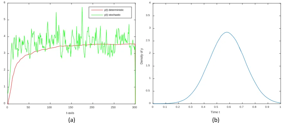
Select α1=α2=0.1, it can be seen from Theorem 3.1 that system (5.1) is sto-chastic ultimate boundedness (See green line in Figure 1(a) and Figure 2(a)). In order to discuss the influence of random white noise, α1=α2 =0 is selected to obtain the deterministic system corresponding to system (5.1), which is ulti-mately bounded (See red line in Figure 1(a) and Figure 2(a)). The blue lines represent the probability density functions of x and y at time 300 (in Figure 1(b)

(11)

[image:11.595.62.538.64.275.2]

Figure 1. System (5.1) take the initial data φ θ

( ) (

= 0.6,0.6

)

, (a) Green line: α α₁= ₂=0.1, red line: α α1= 2=0. (b) The blue line represents the probability functions of x.

Figure 2. System (5.1) take the initial data φ θ

( ) (

= 0.6,0.6

)

, (a) Green line: α α₁= ₂=0.1, red line: α α₁= ₂=0. (b) The blue line represents the probability functions of y.

6. Conclusion

The research of predator-prey system has certainly theory and application value. In this paper, we study a stochastic delayed predator-prey system with Bedding-ton-DeAngelis functional response and discuss some properties of the system solution, which include existence and uniqueness of the global positive solution, stochastic ultimate boundedness of the solution, and asymptotic moment esti-mate. These properties provide a theoretical basis for the management of popu-lation dynamic system. Based on this work, we can also study popupopu-lation dy-namics system with time delay and other types of functional responses.

0 50 100 150 200 250 300

t-axis

0 0.2 0.4 0.6 0.8 1 1.2 1.4

state-axis

x(t) deterministic x(t) stochastic

0 0.1 0.2 0.3 0.4 0.5 0.6 0.7 0.8 0.9 1

Time t

0 0.5 1 1.5 2 2.5 3 3.5 4

Density of x

(a) (b)

0 50 100 150 200 250 300

t-axis

0 1 2 3 4 5 6

state-axis

y(t) deterministic y(t) stochastic

0 0.1 0.2 0.3 0.4 0.5 0.6 0.7 0.8 0.9 1

Time t

0 0.5 1 1.5 2 2.5 3 3.5 4

[image:11.595.64.537.327.534.2]

(12)

Acknowledgements

This work was supported by the National Natural Science Foundation of China (11861027).

Conflicts of Interest

The authors declare no conflicts of interest regarding the publication of this pa-per.

References

[1] Holling, C.S. (1959) The Components of Predation as Revealed by a Study of Small Mammal Predation of the European Pine Sawfly. The Canadian Entomologist, 91, 293-320. https://doi.org/10.4039/Ent91293-5

[2] Holling, C.S. (1959) Some Characteristics of Simple Types of Predation and Parasit-ism. The Canadian Entomologist, 91, 385-395.https://doi.org/10.4039/Ent91385-7

[3] Crowley, P.H. and Martin, E.K. (1989) Functional Response and Interference within and between Year Classes of a Dragonfly Population. Journal of the North Ameri-can Benthological Society, 8, 211-221. https://doi.org/10.2307/1467324

[4] Hassell, M.P. and Varley, C.C. (1969) New Inductive Population Model for Insect Parasites and Its Bearing on Biological Control. Nature, 223, 1133-1137.

https://doi.org/10.1038/2231133a0

[5] Beddington, J.R. (1975) Mutual Interference between Parasites or Predators and Its Effect on Searching Efficiency. Journal of Animal Ecology, 44, 331-341.

https://doi.org/10.2307/3866

[6] DeAngelis, D.L., Goldsten, R.A. and Neill, R. (1975) A Model for Tropic Interac-tion. Ecology, 56, 881-892.https://doi.org/10.2307/1936298

[7] Jost, C. and Arditi, R. (2001) From Pattern to Process: Identifying Predator-Prey Interactions. PopulationEcology, 43, 229-243.

https://doi.org/10.1007/s10144-001-8187-3

[8] Skalski, G.T. and Gilliam, J.F. (2001) Functional Responses with Predator Interfe-rence: Viable Alternatives to the Holling Type II Model. Ecology, 82, 3083-3092.

https://doi.org/10.1890/0012-9658(2001)082[3083:FRWPIV]2.0.CO;2

[9] Gard, T.C. (1984) Persistence in Stochastic Food Web Models. Bulletin of Mathe-matical Biology, 46, 357-370.

[10] Gard, T.C. (1988) Introduction to Stochastic Differential Equations. Dekker, New York.

[11] Mandal, P. and Bnerjee, M. (2012) Stochastic Persistence and Stationary Distribu-tion in a Holling-Tanner Type Prey-Predator Model. Physica A, 391, 1216-1233.

https://doi.org/10.1016/j.physa.2011.10.019

[12] Liu, M. and Wang, K. (2012) Persistence, Extinction and Global Asymptotical Sta-bility of a Non-Autonomous Predator-Prey Model with Random Perturbation. Ap-plied Mathematical Modelling, 36, 5344-5353.

https://doi.org/10.1016/j.apm.2011.12.057

[13] Fan, M. and Kuang, Y. (2008) Dynamics of a Nonautonomous Predator-Prey Sys-tem with the Beddington-DeAngelis Functional Response. Journal of Mathematical Analysis and Applications, 295, 15-39.https://doi.org/10.1016/j.jmaa.2004.02.038

(13)

DOI: 10.4236/ijmnta.2019.84007 105 Int. J. Modern Nonlinear Theory and Application Type with Maturation and Gestation Delays. Nonlinear Analysis: Real World Ap-plications, 11, 4072-4091.https://doi.org/10.1016/j.nonrwa.2010.03.013

[15] Liu, M. and Wang, K. (2012) Global Asymptotic Stability of a Stochastic Lotka-Volterra Model with Infinite Delays, Commun. Communications in Nonlinear Science and Numerical Simulation, 17, 3115-3123. https://doi.org/10.1016/j.cnsns.2011.09.021

[16] Geritz, S. and Gyllenberg, M. (2012) A Mechanistic Derivation of the DeAnge-lis-Beddington Functional Response. Journal of Theoretical Biology, 314, 106-108.

https://doi.org/10.1016/j.jtbi.2012.08.030

[17] Liu, M. and Bai, C. (2014) Global Asymptotic Stability of a Stochastic Delayed Pre-dator-Prey System with Beddington-DeAngelis Functional Response. Applied Ma-thematics and Computation, 226, 581-588.

https://doi.org/10.1016/j.amc.2013.10.052

[18] Mao, X. (1997) Stochastic Differential Equations and Applications. Horwood Pub-lishing, Chichester.