A TOOLBOX FOR FITTING COMPLEX SPATIAL POINT PROCESS MODELS USING INTEGRATED NESTED
LAPLACE APPROXIMATION (INLA)
By Janine B. Illian,
Centre for Research into Ecological and Environmental Modelling, University of St Andrews, Scotland
and
By Sigrunn H. Sørbye,
Department of Mathematics and Statistics, University of Tromsø, Norway
and
By H˚avard Rue
Department of Mathematical Sciences, Norwegian University of Science and Technology, Trondheim, Norway
This paper develops methodology that provides a toolbox for rou-tinely fitting complex models to realistic spatial point pattern data. We consider models that are based on log-Gaussian Cox processes and include local interaction in these by considering constructed co-variates. This enables us to use integrated nested Laplace approxi-mation and to considerably speed up the inferential task. In addition, methods for model comparison and model assessment facilitate the modelling process. The performance of the approach is assessed in a simulation study. To demonstrate the versatility of the approach, models are fitted to two rather different examples, a large rainforest data set with covariates and a point pattern with multiple marks.
1. Introduction.
1.1. Complex point process models. These days a large variety of com-plex statistical models can be fitted routinely to comcom-plex data sets as a result of widely accessible high-level statistical software, such as R (R De-velopment Core Team, 2009) orwinbugs, (Lunn et al., 2000). For instance, the non-specialist user can estimate parameters in generalised linear mixed models or run a Gibbs sampler to fit a model in a Bayesian setting, and expert programming skills are no longer required. Researchers from many
AMS 2000 subject classifications:Primary 60K35, 60K35; secondary 60K35
Keywords and phrases:Cox processes, marked point patterns, model assessment, model comparison
different disciplines are now able to analyse their data with sufficiently com-plex methods rather than resorting to simpler yet non-appropriate methods. In addition, methods for the assessment of a model’s fit as well as for the comparison of different models are widely used in practical applications.
The routine fitting of spatial point process models to complex data sets, however, is still in its infancy. This is despite a rapidly improving technology that facilitates data collection, and a growing awareness of the importance and relevance of small-scale spatial information. Spatially explicit data sets have become increasingly available in many areas of science, including plant ecology (Burslem et al., 2001; Law et al., 2001), animal ecology (Forchham-mer and Boomsma, 1995, 1998), geosciences (Naylor et al., 2009; Ogata, 1999), molecular genetics (Hardy and Vekemans, 2002), evolution (Johnson and Boerlijst, 2002) and game theory (Killingback and Doebeli, 1996) with the aim of answering a similarly broad range of scientific questions. Cur-rently, these data sets are often analysed with methods that do not make full use of the available spatially explicit information. Hence there is a need for making existing point process methodology available to applied scientists by facilitating the fitting of suitable models.
In addition, real data sets are often more complex than the classical data sets that have been analysed with point process methodology in the past. They often consist of the exact spatial locations of the objects or events of interest, and of further information on these objects, i.e. potentially depen-dent qualitative as well as quantitative marks or spatial covariates (Burslem et al., 2001; Moore et al., 2010). There is an interest in fitting complex joint models to the marks (or the covariates) as well as to the point pattern. So far, the statistical literature has discussed few examples of complex point process models of this type.
There have been previous advances in facilitating routine model fitting for spatial point processes, in particular for Gibbs processes. Most markedly, the work by Baddeley and Turner (2000) has facilitated the routine fitting of Gibbs point processes based on an approximation of the pseudolikeli-hood to avoid the issue of intractable normalising constants (Berman and Turner, 1992; Lawson, 1992) as well as the approximate likelihood approach by Huang and Ogata (1999). Work by Baddeley et al. (2005) and Stoyan and Grabarnik (1991) has provided methods for model assessment for some Gibbs processes. Many of these have been made readily available through the libraryspatstat forR(Baddeley and Turner, 2005).
and Turner (2005), Illian and Hendrichsen (2010) include random effects in Gibbs point processes but more complex models, such as hierarchical models or models including quantitative marks, currently cannot be fitted in this framework. Similarly, methods for model comparison or assessment considered in Baddeley et al. (2005) and Stoyan and Grabarnik (1991) are restricted to relatively simple models. Furthermore, both estimation based on maximum likelihood and that based on pseudolikelihood are approximate so that inference is not straight forward. The approximations become less reliable with increasing interaction strength (Baddeley and Turner, 2000).
Cox processes are another, flexible, class of spatial point process mod-els (Møller and Waagepetersen, 2007). Assuming a stochastic spatial trend makes them particularly realistic and relevant in applications. Even though many theoretical results have been discussed in the literature for these (Møller and Waagepetersen, 2004), the practical fitting of Cox point process models to point pattern data remains difficult due to intractable likelihoods. Fitting a Cox process to data is often based on Markov chain Monte Carlo (MCMC) methods. These require expert programming skills and can be very time-consuming both to tune and to run (Møller and Waagepetersen, 2004) so that fitting complex models can easily become computationally pro-hibitive. For simple models, fast minimum contrast approaches to parameter estimation have been discussed (Møller and Waagepetersen, 2007).
However, approaches to routinely fitting Cox process models have been discussed very little in the literature; similarly, methods for model com-parison or assessment for Cox processes have rarely been discussed in the literature (Illian and Rue, 2010; Illian et al., 2011). To the authors’ knowl-edge, Cox processes have not been used outside the statistical literature to answer concrete scientific questions. Within the statistical literature Cox process models have focused on the analysis of relatively small spatial pat-terns in terms of the locations of individual species. Very few attempts have been made at fitting models to both the pattern and the marks (Ho and Stoyan, 2008; Myllym¨aki and Penttinen, 2009), in particular not to patterns with multiple dependent continuous marks and joint models of covariates and patterns have not been considered.
common in other areas of statistics and has become a standard in many ar-eas of application, including methods for model comparison and validation. The approach is based on integrated nested Laplace approximation (INLA) (Rue et al., 2009), which speeds up parameter estimation substantially so that Cox processes can be fitted within feasible time. In order to make the methods accessible to non-specialists, an R package that may be used to run INLA is available and contains generic functions for fitting spatial point process models, seehttp://www.r-inla.org/.
1.2. Cox processes with local spatial structure. Applied researchers are aware that spatial behaviour tends to vary at a number of spatial scales as a result of different underlying mechanisms that drive the pattern (Wiegand et al., 2007; Latimer et al., 2009). Local spatial behaviour is often of specific interest but the spatial structure also varies on a larger spatial scale due to the influence of observed or unobserved spatial covariates. Cox processes model spatial patterns relative to observed or unobserved spatial trends and would be ideal models for these data sets.
However, Cox processes typically do not consider spatial structures at different spatial scales within the same model. More specifically, a specific strength of spatial point process models is their ability to take into account detailed information at very small spatial scales contained in spatial point pattern data, in terms of the local structure formed by an individual and its neighbours. So far, Cox processes have often been used to relate the lo-cations of individuals to environmental variation, phenomena that typically operate on larger spatial scales. However, different mechanisms operate at a smaller spatial scale. Spatial point data sets are often collected with a spe-cific interest in the local behaviour of individuals, such as spatial interaction or local clustering (Law et al., 2001; Latimer et al., 2009).
We consider an approach to fitting Cox process models that reflect both the local spatial structure and spatial behaviour at a larger spatial scale by using a constructed covariate together with spatial effects that account for spatial behaviour at different spatial scales. This approach is assessed in a simulation study and we also discuss issues specific to this approach that arise when several spatial scales are accounted for in a model.
covariate and fits this to a rainforest data set. A hierarchical approach is considered in Section 5, where both (multiple) marks and the underlying pattern are included in a joint model and fitted to a data set of eucalyptus trees and koalas foraging on these trees.
2. Methods.
2.1. Spatial point process models. Spatial point processes have been dis-cussed in detail in the literature, see Stoyan et al. (1995), van Lieshout (2000), Diggle (2003), Møller and Waagepetersen (2004, 2007) and Illian et al. (2008). Here we aim at modelling a spatial point patternx= (ξ1, . . . , ξn), regarding it as a realisation from a spatial point processX. For simplicity we consider only point processes in R2 but the approaches can be generalised to point patterns in higher dimensions.
We refer the reader to the literature for information on different (classes of) spatial point process models such as the simple Poisson process, the stan-dard null model of complete spatial randomness, as well as the rich class of Gibbs (or Markov) processes (van Lieshout, 2000). Here, we discuss the class of Cox processes, in particular log-Gaussian Cox processes. Cox processes lend themselves well to modelling spatial point pattern data with spatially varying environmental conditions (Møller and Waagepetersen, 2007) as they model spatial patterns based on an underlying (or latent) random field Λ(·) that describes the random intensity, assuming independence given this field. In other words, given the random field, the point pattern forms a Poisson process. Log-Gaussian Cox processes as considered for example in Møller et al. (1998) and Møller and Waagepetersen (2004, 2007), are a particularly flexible class, where Λ(s) has the form Λ(s) = exp{Z(s)}, and {Z(s)} is a Gaussian random field, s ∈ R2. Other examples of Cox processes include shot-noise Cox processes (Møller and Waagepetersen, 2004).
Here, we consider a general class of complex spatial point process models based on log-Gaussian Cox processes that allows the joint modelling of spa-tial patterns along with marks and covariates. We include both small and larger scale spatial behaviour, using a constructed covariate and additional spatial effects. The resulting models can be regarded as latent Gaussian models and hence INLA can be used for parameter estimation and model fitting.
(2009) show that if ζ has a sparse precision matrix and the number of hy-perparameters is small (i.e.≤7), inference based on INLA is fast.
The main aim of the INLA approach is to approximate the posteriors of interest, i.e. the marginal posteriors for the latent field π(ζi|y),and the marginal posteriors for the hyperparameters π(θj|y), and use these to cal-culate posterior means, variances etc. These posteriors can be written as
π(ζi|y) =
Z
π(ζi|θ,y)π(θ|y)dθ (2.1)
π(θj|y) =
Z
π(θ|y)dθ−j. (2.2)
The nested formulation is used to computeπ(ζi|y) by approximatingπ(ζi|θ,y) and π(θ|y), and then to use numerical integration to integrate out θ. This is feasible, since the dimension ofθ is small. Similarly,π(θj|y) is calculated by approximating π(θ|y) and integrating outθ−j.
The marginal posterior in equations (2.1) and (2.2) can be calculated using the Laplace approximation
˜
π(θ|y)∝ π(ζ, θ,y) ˜
πG(ζ|θ,y)
ζ=ζ∗(θ)
where ˜πG(ζ|θ,y) is the Gaussian approximation to the full conditional ofζ, andζ∗(θ) is the mode of the full conditional forζ, for a given θ. This makes sense, since the full conditional of a zero mean Gauss Markov random field can often be well approximated by a Gaussian distribution by matching the mode and the curvature at the mode (Rue and Held, 2005). Further details are given in Rue et al. (2009) who show that the nested approach yields a very accurate approximation if applied to latent Gaussian models. As a result, the time required for fitting these models is substantially reduced.
2.3. Fitting log-Gaussian Cox processes with INLA. The class of latent Gaussian models comprises log-Gaussian Cox processes and hence the INLA approach may be applied to fit these. Specifically, the observation window is discretised intoN =nrow×ncol grid cells{sij}, each with area |sij|,i= 1, . . . , nrow, j = 1, . . . , ncol. The points in the pattern can then be described by {ξijkij} with kij = 1, . . . , yij, where yij denotes the observed number of
points in grid cell sij. We condition on the point pattern and conditionally onηij =Z(sij) we have
(2.3) yij|ηij ∼P o(|sij|exp(ηij)),
We modelηij as
(2.4) ηij =β0+f(zc(sij)) +f1s(sij) +. . .+fps(sij) +uij,
where the functions f1s(sij) +. . .+fps(sij) are spatially structured effects that reflect large scale spatial variation in the pattern. These effects are modelled using a second-order random walk on a lattice, using vague gamma priors for the hyperparameter and constrained to sum to zero (Rue and Held, 2005). In the models that we discuss below, the spatially structured effects relate to observed and unobserved spatial covariates as discussed in the examples in Sections 4 and 5. Including spatial covariates directly in the model as fixed effects in addition to the random effects is straight forward. For simplicity we omit these in equation (2.4) since this is not relevant in the specific data sets and models discussed below. uij denotes a spatially unstructured zero-mean Gaussian i.i.d. error term, using a gamma prior for the precision.
Further, zc(sij) denotes a constructed covariate. Constructed covariates are summary characteristics defined for any location in the observation win-dow reflecting inter-individual spatial behaviour such as local interaction or competition. We assume that this behaviour operates at a smaller spatial scale than spatial aggregation due to (observed or unobserved) spatial co-variates and hence the spatially structured effects. The use of constructed covariates yields models with local spatial interaction within the flexible class of log-Gaussian Cox process models. It avoids issues with intractable normalising constants that are common in the context of Gibbs processes (Møller and Waagepetersen, 2004), since the covariates operate directly on the intensity of the pattern rather than on the density or the conditional intensity (Schoenberg, 2005).
The functional relationship between the outcome variable and the con-structed covariate is typically not obvious and might often not be linear. We thus estimate this relationship explicitly by a smooth functionf(zc(sij)) and inspect this estimate to gain further information on the form of the spatial dependence. This function will be modelled as a first-order random walk, also constrained to sum to zero.
The constructed covariate considered in this paper is based on the nearest point distance, which is simple and fast to compute. Specifically, for each centre point of the grid cells we find the distance to the nearest point in the pattern outside this grid cell, as
(2.5) zc(sij) =d(sij) = min ξl∈x\sij
wherecij denotes the centre point of cellsij andk · kdenotes the Euclidean distance. Defined this way, the constructed covariate can be used both to model local repulsion and local clustering.
During the modelling process, methods for model comparison based on the deviance information criterion (DIC) (Spiegelhalter et al., 2002), may be used to compare different models with different levels of complexity. Fur-thermore, both the (estimated) spatially structured field and the error field in (2.4) may be used to assess the model fit. The spatially structured effect may be used to reveal remaining spatial structured that is unexplained by the current model and the unstructured effects may be interpreted as a spa-tial residual. This provides a method for model assessment akin to residuals in, e.g. linear models.
This approach yields a toolbox for fitting, comparing and assessing realis-tically complex models of spatial point pattern data. We show that different types of flexible models can be fitted to point pattern data with complex structures using the INLA approach within reasonable computation time. This includes joint models of large point patterns and covariates operating on a large spatial scale and local clustering (Section 4) as well as of a pattern with several dependent marks which also depend on the pattern (Section 5).
2.4. Issues of spatial scale. In the natural world, different mechanisms operate at different spatial scales (Steffan-Dewenter et al., 2002) and hence are reflected in a spatial pattern at these scales. It is crucial to bear this in mind during the analysis of spatial data derived from nature, including spa-tial point pattern data. Some mechanisms such as seed dispersal in plants or territorial behaviour in animals may operate at a local spatial scale, while others, such as aggregation resulting from an association with certain envi-ronmental covariates, operate on the scale of the variation in these covariates and hence often on a larger spatial scale. In addition, a spatial scale that is relevant in one application may not be relevant for a different data set. Hence the analysis of a spatial point pattern always involves a consideration of the appropriate spatial scales at which mechanisms of interest may op-erate, regardless of the concrete analysis methods. Even as early as at the outset of a study, when an appropriately sized observation window has to be chosen, relevant spatial scales operating in the system of interest have to be taken into consideration.
knowledge (such as existing data on dispersal distances in plants or the sizes of home ranges in territorial animals) or common sense.
In the models we discuss here, we explicitly take mechanisms operating at several different scales into account and have to choose these sensibly, based on knowledge of the systems. The spatially structured effect reflects spatial autocorrelation at a large spatial scale whereas the constructed covariate is used to describe small scale inter-individual behaviour. In addition, since we grid the data in this approach the number of grid cells clearly determines the spatial resolution, especially at a small scale and is clearly linked to computational costs and the extent to which information is lost through gridding the data. In the following, we discuss issues related to each of these three parts of the models where spatial scale is relevant.
A spatially structured effect is typically included in a spatial model as a spatially structured error term, i.e. in order to account for any spatial auto-correlation unexplained by covariates in the model. INLA currently supports the 2nd order random walk on a lattice as a model for this, with a gamma prior for the variance of the spatially structured effect. The choice of this prior determines the smoothness of the spatial effect and through this, the spatial scale at which it operates. This prior has to be chosen carefully to avoid overfitting. This is particularly crucial in the context of spatial point patterns with relatively small numbers of points, where the gridded data are typically rather sparse (Illian et al., 2011). If the spatial effect is chosen to be too coarse, it explains the spatial variation at too small a scale resulting in a coarse estimate of the spatially structured effect. This estimate would perfectly explain every single data point resulting in overfitting rather than in a model of a generally interpretable trend. Given the role of the spatially structured effect, it appears plausible to choose the prior so that the spa-tial effect operates at a similar spaspa-tial scale as the covariate. Problems can occur when the spatially structured effect operates at a smaller scale than the covariate as it is then likely to explain the data better than the covari-ates, rendering the model rather useless. In the absence of covariate data, background knowledge on spatial scales may aid in choosing the prior.
The choice of prior for the spatially structured effect is strongly related to the choice of grid size. However, in our experience the overall results often do not change substantially when the grid size was varied within reason. In applications, the locations of the modelled objects as well as spatial covari-ates are sometimes given on a grid with a fixed resolution. We recommend using a grid that is not finer than that given by the data in the analysis.
3. Using a constructed covariate to account for local spatial structure – a simulation study. In Section 4 we use a constructed co-variate primarily to incorporate local spatial structure into a model, while accounting for spatial variation at a larger spatial scale. To illustrate the use of the given constructed covariate and to assess the performance of the resulting models, we simulate point patterns from various classical point-process models. Note, however, that we do not aim at explicitly estimating the parameters of these models but at assessing (i) whether known spatial structures may be detected through the use of the constructed covariate, as suggested here, and (ii) whether simulations from the fitted models generate patterns with similar characteristics. In the applications we have in mind, such as those discussed in the example in Section 4, the data structure is typically more complicated.
For the purpose of this simulation study we consider three different situ-ations: patterns with local repulsion (Section 3.1), patterns with local clus-tering (Section 3.2) and patterns with local clusclus-tering in the presence of a larger-scale spatial trend (Section 3.3). We generate example patterns from different point process models with these properties on the unit square. For all simulations results this observation window has been discretized into a 100×100 grid.
In Sections 3.1 and 3.2 we initially assume that there is no large-scale spatial variation, with the aim of inspecting only the constructed covariate and we consider
(3.1) ηij =β0+f(zc(sij)),
using the notation in Section 2.3. In Section 3.3 we consider both small-and large-scale spatial structures by including a spatially structured effect
fs(sij) in addition to the constructed covariatezc(sij) and
(3.2) ηij =β0+f(zc(sij)) +fs(sij).
characteristics of the simulated patterns with the generated example pat-terns. More specifically, for i= 1, . . . , nrow and j = 1, . . . , ncol, denote the joint distribution ofy={yij}given the latent field η={ηij}, by
p(y|η) =Y i,j
p(yij |ηij) =
Y
i,j
exp(−λij)
λyij
ij
yij!
,
where the mean λij = |sij|exp(ηij). For a given example pattern, we first apply INLA to find the estimate ˆηof the latent field for all grid cells. To eval-uate the estimated function of the constructed covariate for all arguments, we apply thesplinefuncommand in R to perform cubic spline interpolation of the original data points. Using the Metropolis algorithm, we assume an initial pattern x(0), which is randomly scattered in the unit square, having the same number of points as the original pattern. The kth step of the al-gorithm is performed by randomly selecting one point of the patternx(k−1)
and propose to move this point to a new position drawn uniformly in the unit square. The proposal is accepted with probability
α= min 1, p(y
(k)|ηˆ)
p(y(k−1)|ηˆ)
!
, k= 1,2, . . .
where y(k) denotes the resulting grid cell counts for x(k). The simulated patterns in Sections 3.1 – 3.3 each result from 100,000 iterations of the algorithm.
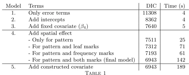
The pattern resulting from the Metropolis–Hastings algorithm (Figure 1 (d)) shows very similar characteristics to those in the original pattern. This indicates that the model based on the nearest point constructed covariate in equation (2.5) captures adequately the spatial information contained in the repulsive pattern.
The estimatedL-function (Besag, 1977), for the simulated pattern and the original pattern confirm this impression, as they look very similar (Figure 1 (e)). Additionally, we have calculated simulation envelopes for theL-function of Strauss processes with the given parameter values, using 50 simulated patterns and 100 000 iterations of the Metropolis algorithm for each pattern (Figure 1 (f)). We notice that the estimated L-functions of the orignial patterns are well within the simulation envelopes for all distances.
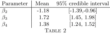
3.2. Modelling clustering. In order to assess the performance of the model in (3.1) in the context of clustered patterns, we generate patterns from a homogeneous Thomas process (Neyman and Scott, 1952) in the unit square, with parametersκ= 10 (the intensity of the Poisson process of cluster cen-tres), σ = 0.05 (the standard deviation of the distance of a process point from the cluster centre) andµ= 50 (the expected number of points per clus-ter) (see Figure 2 (a) for an example). We fit the model in equation (3.1) using the constructed covariate in (2.5) (Figure 2 (b)). The shape of the estimated functional relationship between the constructed covariate and the outcome variable (Figure 2 (c)) now indicates that the intensity is negatively related to the value of the constructed covariate as the intensities increase for smaller distances, reflecting local clustering. At larger distances (>0.1) the function levels out, indicating that at these distances the covariate and the intensity are unrelated.
The pattern simulated from the fitted model (Figure 2 (d)) shows that the constructed covariate introduces some clustering in the model. However, the resulting pattern shows fewer and less distinct clusters than the original pattern. Similarly, the estimatedL-function for the pattern simulated from the fitted model shows a weaker local clustering effect than the original pattern (Figure 2 (e)). This is also illustrated by the simulation envelopes for 50 patterns of the fitted model which do not include the trueL-function (Figure 2 (f)).
ag-gregation at a larger spatial scale, e.g. due to dependence on underlying observed or unobserved covariates. Hence the main reason for using con-structed covariates in the data example in Section 4 is to distinguish be-haviour at different spatial resolutions, in order to provide information on mechanisms operating at different spatial scales.
We illustrate the use of constructed covariates in this context by generat-ing an inhomogeneous, locally clustered pattern mimickgenerat-ing a situation where different mechanisms have caused local clustering and large scale inhomo-geneity. In applications, the inhomogeneity may be modelled using suitable spatially varying covariates or assuming an unobserved spatial variation or both. We generate patterns from an inhomogeneous Thomas process with parametersσ= 0.01 andµ= 5 and a simple trend function for the intensity of parent points given by κ(x1, x2) = 50x1. Each pattern is then super-imposed with a pattern generated from an inhomogeneous Poisson process with trend functionλ=x1/4 (Figure 3 (a)).
We again use the constructed covariate in (2.5), see Figure 3 (b), and fit the model in (3.2). The inspection of the functional relationship between the constructed covariate and the outcome (Figure 3 (c)) shows that at small values of the covariate the intensity is negatively related to the constructed covariate, reflecting clustering at smaller distances. The estimated spatially structured effect picks up the larger-scale spatial behaviour (Figure 3 (d)). Patterns simulated from the fitted model look quite similar to the original pattern (Figure 3 (e)) However, local clustering is slightly stronger in the original pattern than in the simulated pattern (Figure 3 (f)).
This is again confirmed by the simulation envelopes for the simulated patterns from the fitted model, as shown in Figure 4. The mean estimated L-function for the generated patterns is very close to the upper edge of the simulation envelops and partly outside, indicating that the fitted model does not reflect the strength of clustering sufficiently well.
the results shown here are typical examples. We have run simulations from the same models as above with different sets of parameters and have obtained essentially the same results. Further, fitting the model in equation (3.1) to patterns simulated from a homogeneous Poisson process resulted in a non-significant functional relationship, i.e. the modelling approach does not pick up spurious clustering or regularity.
The approach allows us to fit models that take into account small-scale spatial behaviour, regularity as well as clustering, in the context of log-Gaussian Cox processes, i.e. as latent log-Gaussian models. Since these can be fitted using the INLA approach, fitting is fast and exact. In addition, we avoid some of the typical problems that arise with Gibbs process models, i.e. we do not face issues of intractable normalising constants, and regular as well as clustered patterns may be modelled.
However, the simulation also shows that the approach of using constructed covariates works clearly better with repulsive patterns than with clustered patterns. This is akin to similar issues with Gibbs processes, where repulsive patterns are less problematic to model than clustered patterns. Certainly, this is related to the fact that it is difficult to tell apart clustering from in-homogeneity (Diggle, 2003). When working with constructed covariates the issues highlighted, i.e. that local clustering may have been underestimated have to be taken into account, especially in the interpretation of results.
that are defined only for the points in the pattern and include these in the model.
Distinguishing spatial behaviour at different spatial scales is clearly an ill-posed problem, since the behaviour at one spatial scale is not independent of that at different spatial scales (Diggle, 2003). The approach we take here will not always be able to distinguish clustering at different scales. However, different mechanisms that operate at very similar spatial scales are likely to be non-identifiable by any method, irrespective of the choice of model or the constructed covariate. Constructed covariates hence only provide useful results when the processes they are meant to describe operate at a spatial scale that is distinctly smaller than the larger scale processes in the same model.
Admittedly, the use of constructed covariates is of a rather subjective and ad hoc nature. Clearly, in applications the covariates have to be con-structed carefully, depending on the questions of interest; different types of constructed covariates may be suitable in different contexts. However, sim-ilarly subjective decisions are usually made when a model is fitted that is purely based on empirical covariates, as these have been specifically chosen as potentially influencing the outcome variable, based on background knowl-edge. In addition, due to the apparent danger of overfitting, constructed covariates should only be used if there is an interest in the local spatial behaviour in a specific data set and if there is reason to believe that small-and large-scale spatial behaviour are operating at scales that are different enough to make them identifiable.
4. Joint model of a point pattern and environmental covariates.
4.1. Modelling approach. In this example we consider a point pattern
Waagepetersen (2007); Waagepetersen and Guan (2009). In addition, it is less clear for soil variables than for topography covariates if these influence the presence of trees, or whether the presence of trees impacts on the soil variables. Whereas models in which the soil variables are considered fixed and not modelled alongside the pattern, the model we deal with here does not make any assumption on the direction of this influence.
As a result, we suggest a joint model of the covariates along with the pattern that uses the original (non-interpolated) data on the covariates and accounts for measurement error. I.e. we fit the model in equation (2.4) to
x and jointly fit a model to the covariates. The pattern and the covariates are linked by joint spatial fields. An additional spatially structured effect is used to detect any remaining spatial structures in the pattern that cannot be explained by the joint fields with the covariates.
In the case of p = 2 we fit the following model, where the pattern is modelled as
(4.1) ηij =β0+f(zc(sij)) +fs(sij) +gs(sij) +hs(sij),
and the covariates as
(4.2) z1ij =fs(sij) +uij,
and
(4.3) z2ij =gs(sij) +vij,
wherez1ij andz2ij are the observed covariates in grid cells where the covari-ates have been measured and missing where they have not been measured.
f(zc(sij)) represents the function of the constructed covariate (2.5). fs(.) and gs(.) are spatially structured effects, i.e. reflect a random field for each of the covariates andhs(.) reflects spatial autocorrelation in the pattern un-explained by the covariates;uij andvij are spatially unstructured fields used to account for measurement or sampling error.
In addition to the spatial effect reflecting the empirical covariates, which are likely to have an impact on the larger scale spatial behaviour, we use the constructed covariate to account for local clustering. In the application we have in mind (see Section 4.2) this clustering is a result of seed-dispersal mechanisms operating on a much smaller spatial scale than that the aggre-gation of individuals due to an association with environmental covariates.
4.2.1. The rainforest data. Some extraordinarily detailed multi-species maps are being collected in tropical forests as part of an international effort to gain greater understanding of these ecosystems (Condit, 1998; Hubbell et al., 1999; Burslem et al., 2001; Hubbell et al., 2005). These data comprise the locations of all trees with diameters at breast height (dbh) 1 cm or greater, a measure of the size of the trees (dbh), and the species identity of the trees. The data usually amount to several hundred thousand trees in large (25 ha or 50 ha) plots that have not been subject to any sustained disturbance such as logging. The spatial distribution of these trees is likely to be determined by both spatially varying environmental conditions and local dispersal.
Recently, spatial point process methodology has been applied to analyse some of these data sets (Law et al., 2009; Wiegand et al., 2007) using non-parametric descriptive methods as well as explicit models (Waagepetersen, 2007; Guan, 2008; Waagepetersen and Guan, 2009; Yue and Loh, 2011). Rue et al. (2009) model the spatial pattern formed by a tropical rain forest tree species on the underlying environmental conditions and use the INLA approach to fit the model.
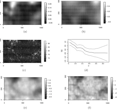
We analyse a data set that is similar to those discussed in the above references. Since the spatial structure in a forest reflects dispersal mech-anisms as well as association with environmental conditions, we include a constructed covariate to account for local clustering. The model is fitted to a data set from a 50 ha forest dynamics plot at Pasoh Forest Reserve, Penin-sular Malaysia. This study focuses on the species Aporusa microstachya consisting of 7416 individuals (Figure 5 (a)). The environmental covariates have been observed in 83 locations that are distinct from the locations of the trees (Figure 5 (b)). The plot lies in a forest that has never been logged with very narrow streams on almost flat land. The data collected in 1995 are used here when the plot contained 320903 stems from 817 species. The species is the most common small tree on the plot. It is of interest if this species, as an aluminium accumulator, covaries with magnesium availability as aluminium uptake might constrain its capacity to take up nutrient cations such as magnesium. In addition, its covariation with phosphorus is consid-ered here as the element is thought to be the nutrient primarily limiting forest productivity and individual tree growth in tropical forests (Burslem, personal communication, February 2011).
magne-siumgs(.), are displayed in Figure 6 (a) and (b). We notice that these effects are very smooth but we have to remember that the covariate information is sparse and only available in 83 grid cells. In terms of DIC, the empirical co-variate terms explain some spatial structure of the pattern as DIC increases from 15379 to 15440 if these two terms are not included. High phosphorus seems to coincide with low tree density and a similar, but less clear, pattern emerges for magnesium. Currently, the ecological literature cannot explain these results, but they could be related to resource partitioning along axes of soil nutrient availability (Burslem, personal communication, September 2011, John et al. (2007)). In addition, it is currently also unclear if the soil properties cause an aggregation of trees, as they provide suitable growing conditions, or whether a high tree intensity leads to low levels of magnesium or phosphorus resulting from the chemical composition of the leaf litter.
The plot of the constructed covariate in Figure 6 (c) illustrates the res-olution of the local clustering represented by it. The resulting estimated function of the constructed covariate is shown in Figure 6 (d), which indi-cates that it accounts for clustering of up to a distance of 15 metres. The estimated spatial effect hs(.) for the pattern is given in Figure 6 (e) while Figure 6 (f) displays the estimated spatially structured effect if the con-structed covariate is left out of the full model. This last figure shows clear local structure in the spatial effect and might give a model which is over-fitted to the actual pattern. Including the constructed covariate, the local structure of the spatial effect is removed making the spatial effect smoother. This indicates that spatial behaviour at a local scale has been picked up by the constructed covariate. In this way the model can account for spatial structures at different scales. The two unstructured spatial fields in Equa-tions (4.2) and (4.3) do not show any particular pattern (results not shown). Fitting this model took 55 minutes to run (2.66 GHz Intel Core i7 processor).
assumed to be known everywhere and fixed. In many typical applications, however, the values of spatial covariates in the location of the points forming the point process are not known. Similarly, the direction of the relationship between soil properties and tree presence may be not clear. We generalise the approach in Rue et al. (2009) here and fit a joint model of the pattern and the covariates. This approach distinguishes between locations where the values of the covariates are available but potentially subject to measurement error and those where they are not. In addition, it does not assume that the soil variables impact on the pattern but not vice versa. We also consider a constructed covariate that reflects local clustering as a result of local seed dispersal, as discussed above.
The given approach accommodates model comparison and model assess-ment, both of which are of practical value in many applications. An inspec-tion of the estimated spatially structured effect in Figure 6 (e) indicates that some spatial structure still remains in the point pattern which cannot be ex-plained by the current model, i.e. the current model can still be improved on. Hence, judging by the Figure 6 (e) it might be possible to improve the model by including further covariates and the structure of the estimated spa-tial effect might be used to suggest a suitable covariate. Previous approaches to fitting a model to these data (Waagepetersen, 2007; Waagepetersen and Guan, 2009) neither have been able to reveal the shortcomings of the models nor to provide mechanisms that help identify covariates that might improve the model.
The function of constructed covariate (Figure 6 (d)), which reflects local clustering up to a distance of 15 metres may be interpreted as a seed dis-persal kernel. Biological research has shown that this species is likely to be dispersed primarily by small understorey birds that feed in the canopy and mostly drop the seeds beneath the parent tree. Since trees of the species Aporusa microstachyathese are relatively small 15 m reflect the maximum radius of the tree crown (Burslem et al., 2001).
The approach discussed here can be extended easily to allow more com-plex models to be fitted, such as a model of both the spatial pattern and associated marks, along the lines of the model discussed in Section 5. For instance, this may include a model of both the spatial pattern and the size and the growth of the trees. Here, both size and growth might depend on the spatial pattern and growth might also depend on size.
a gross over-simplification for many systems. In practice, researchers hence often collect data on the locations of the individuals along with data on additional properties, i.e. marks. In this section we discuss a marked point pattern with several dependent marks, which also depend on the spatial pattern, and consider a joint model of the marks and the pattern. Models where marks depend on the point pattern have recently been considered in the literature (Menezes, 2005; Ho and Stoyan, 2008; Myllym¨aki and Pent-tinen, 2009). Also note the work by Diggle et al. (2010), where a point process with intensity dependent marks is used in the context of preferential sampling in geostatistics. The model we fit here is more general than these related models, since we model multiple dependent marks jointly with the pattern.
5.1. Data structure and modelling approach. We analyse a spatial point patternx= (ξ1, . . . , ξn) together with several types of nonindependent asso-ciated marks. We consider only two marksm1 = (m11, . . . , m1n) and m2 = (m21, . . . , m2n) here but the approach can be generalised in a straightforward way to include more than two marks. Them1 are assumed to follow an ex-ponential family distributionF1θ1 with parameter vectorθ1= (θ11, . . . , θ1q)
and to depend on the intensity of the point pattern, while the m2 are as-sumed to follow a (different) exponential family distribution F2θ2 with
pa-rameter vector θ2 = (θ21, . . . , θ2q) and to depend both on the intensity of the point pattern and on the marksm1. Without loss of generality, the pa-rametersθ11andθ21are the location parameters of the distributionsF1and
F2, respectively.
We discretise the observation window as discussed in Section 2.3, and for the spatial pattern we assume the model
(5.1) ηij =β01+f(zc(sij)) +β1·fs(sij) +uij,
using the same notation as in (2.4). For the marks, we construct a model where the marksm1 depend on the pattern by assuming that they depend on the same spatially structured effect fs(sij). Specifically, we assume that
m1(ξijkij)|κijkij ∼F1θ1(κijkij, θ12, . . . , θ1q) with
(5.2) κijkij =β02+β2·fs(sij) +vijkij,
where vijkij is another error term. The marks m2 are assumed to depend
both on the spatial pattern through fs(sij) and on the marks m1. We thus have thatm2(ξijkij)|νijkij ∼F2θ2(νijkij, θ22, . . . , θ2q) with
(5.3) νijkij =β03+β3·fs(sij) +β4·m1(ξijkij) +wijkij,
5.2. Application to example data set.
5.2.1. Koala data. Koalas are arboreal marsupial herbivores native to Australia with a very low metabolic rate. They rest motionless for about 18 to 20 hours a day, sleeping most of that time. They feed selectively and live almost entirely on eucalyptus leaves. Whereas these leaves are poisonous to most other species, the koala gut has adapted to digest them. It is likely that the animals preferentially forage leaves that are high in nutrients and low in toxins as an extreme example of evolutionary adaptation. An understanding of the koala-eucalyptus interaction is crucial for conservation efforts (Moore et al., 2010).
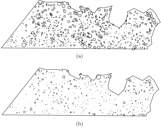
The data have been collected in a study conducted at the Koala Con-servation Centre on Phillip Island, near Melbourne, Australia. For each of 915 trees within a reserve enclosed by a koala-proof fence (Figure 7), infor-mation on the leaf chemistry and on the frequency of koala visits has been collected. The leaf chemistry is summarised in a measure of the palatability of the leaves (”leaf mark” mL). Palatability is assumed to depend on the intensity of the point pattern. In addition, ”frequency mark”mF describe for each tree the diurnal tree use by individual koalas collected at monthly intervals between 1993 and March 2004. ThemF are assumed to depend on the intensity of the point pattern as well as on the leaf marks.
There are no additional covariate data available for the given data set. Hence for the locations of the trees we use the model in (5.1) with notation as above. For the leaf and frequency marks we use the models in equa-tions (5.2) and (5.3), respectively. The leaf marks are assumed to follow a normal distribution and the frequency marks a Poisson distribution, i.e.
mL(ξijkij)|κijkij ∼N(κijkij, σ
2) and m
F(ξijkij)|νijkij ∼P o(exp(νijkij)).
5.2.2. Results. With these distributional assumptions for the marks, we fit a joint model as given in equations (5.1) - (5.3) to the data set. The results are based on an observation window discretised into 1571 grid cells. In order to fit spatial effects we embed this area within a rectangular area. For the constructed covariate, we perform a simple edge correction for the distances in (2.5), assuming missing values in grid cells in which the distance from the centre point to the border is shorter than the nearest-point distance.
pat-Model Terms DIC Time (s)
1. Only error terms 11308 4
2. Add intercepts 8362 4
3. Add fixed covariate (β4) 7640 5
4. Add spatial effect
- Only for pattern 7511 25
- For pattern and leaf marks 7312 71
- For pattern and frequency marks 7193 61 - For pattern and both marks (final model) 6943 142
[image:22.612.149.458.109.232.2]5. Add constructed covariate 6943 189
Table 1
DIC values and computation time for different fitted models for the koala data.
tern together with one or both of the two marks, in which DIC decreases to 6943. Inclusion of the constructed covariate in (5.1) does not improve the model fitting for this data set. This is not surprising as the original pattern does not seem to exhibit any strong local clustering effect and as a result the estimated function of the constructed covariate is not significantly different from 0.
The estimated common spatial effect (Figure 8 (a)), represents spatial autocorrelation present in the pattern and the marks which might be the result of related environmental processes such as nutrient levels in the soil. The estimated parameter value forβ2 andβ3 have opposite signs (Table 2). The negative sign forβ2 indicates that palatability is low where the trees are aggregated, which might have been caused by competition for soil nutrients in these areas. The positive sign forβ3reflects that the koalas are more likely to be present in areas with higher intensity. Recalling that the data have been accumulated over time, this might be due to the koalas being more likely to change from one tree to a neighbouring tree where the trees are aggregated. The mean of the posterior density for the parameter β4 in the final model is 1.38, indicating a significant positive influence of palatability on the frequency of koala visits to the trees. The three unstructured terms are given in Figure 8 (b) - (d). A slight trend in the residuals for the leaf marks may be observed in Figure 8 (c) with lower values towards the bottom left probably reflecting an inhomogeneity that cannot be accounted for by the joint spatial effectfs(sij).
Parameter Mean 95% credible interval
β2 -1.18 [-1.39,-0.96]
β3 1.72 [1.45, 1.98]
β4 1.38 [1.24, 1.52]
[image:23.612.216.393.113.168.2]Table 2
Posterior means and95% credible intervals for parameters in the koala model.
model of the marks which implicitly takes the spatial dependence into ac-count by modelling it alongside the marks. The model we use here is similar to approaches taken in Menezes (2005); Ho and Stoyan (2008); Myllym¨aki and Penttinen (2009). Since our approach is very flexible, it can easily be generalised to allow for separate spatially structured effects for the pattern and the marks and to include additional empirical covariates; these have not been available here. Hence, using the approach considered here, we are able to fit easily a complex spatial point process model to a marked point pattern and to assess its suitability for a specific data set.
Marked point pattern data sets where data on marks are likely to depend on an underlying spatial pattern are not uncommon. Within ecology, for instance, metapopulation data (Hanski and Gilpin, 1997) typically consist of the locations of sub-populations and their properties, and have a similar structure to the data set considered here. These data sets may be modelled using a similar approach and it is straightforward to fit related but more complex models, including empirical covariates or temporal replicates. Sim-ilarly, marks are available for the rainforest data discussed in Section 4. As mentioned there, a model that includes the marks of the trees may also be fitted using the approach discussed here.
6. Discussion. Researchers outside the statistical community have be-come familiar with fitting a large range of different models to complex data sets using software available inR.
This paper provides a very flexible framework for routinely fitting models to complex spatial point pattern data with little computational effort using models that account for both local and global spatial behaviour. We consider complex data examples and demonstrate how marks as well as covariates can be included in a joint model. I.e. we consider a situation where the marks and the covariates can be modelled along with the pattern and show that it is computationally feasible to do so. We can take account of local spatial structure by using a constructed covariate, which we discuss in detail in Section 3.
fitting of other even more complex models. It is feasible to fit several related models to realistically complex data sets if necessary, and to use the DIC to aid the choice of covariates. The posterior distributions of the estimated parameters can be used to assess the significance of the influence of differ-ent covariates in the models. Through the use of a structured spatial effect and an unstructured spatial effect it is possible to assess the quality of the model fit. Specifically, the structured spatial effect can be used to reveal spatial correlations in the data that have not been explained with the co-variates and may help researchers identify suitable coco-variates to incorporate into the model. Spatially unstructured effects may be used to account for and identify extreme observations such as locations where covariate values have been collected with a particularly strong measurement error.
There is an extensive literature on descriptive and non-parametric ap-proaches to the analysis of spatial point patterns, specifically on (functional) summary characteristics describing first and second order spatial behaviour, in particular on Ripley’sK-function (Ripley, 1976) and the pair correlation function (Stoyan et al., 1995). In both the statistical and the applied liter-ature these have been discussed far more frequently than likelihood based modelling approaches and provide an elegant means for characterising the properties of spatial patterns (Illian et al., 2008). A thorough analysis of a spatial point pattern typically includes an extensive exploratory analysis and in many cases it may even seem unnecessary to continue the analysis and fit a spatial point process model to a pattern. An exploratory analysis based on functional summary characteristics such as Ripley’sK–function or the pair-correlation function considers spatial behaviour at a multitude of spatial scales, making this approach particularly appealing. However, with increasing complexity of the data, it becomes less obvious how suitable sum-mary characteristics should be defined for these, and a point process model may be a suitable alternative. For example, it is not obvious how one would jointly analyse the two different marks together with the pattern in the koala data set based on summary characteristics. However, as discussed in Section 5, it is straightforward to do this with a hierarchical model. In addition, most exploratory analysis tools assume the process to be first-order stationary or at least second-order reweighted stationary (Baddeley et al. 2000) – a situa-tion that is both rare and difficult to assess in applicasitua-tions, in particular in the context of realistic and complex data sets. The approach discussed here does not make any assumptions about stationarity but explicitly includes spatial trends into the model.
Gibbs process model as a parametric or non-parametric, yet deterministic, trend, while it is treated as a stochastic process in itself here. Modelling the spatial trend in a Gibbs process hence often assumes that an explicit and deterministic model of the trend as a function of location (and spatial co-variates) is known (Baddeley and Turner, 2005). Even in the non-parametric situation, the estimated values of the underlying spatial trend are consid-ered fixed values, which are subject neither to stochastic variation nor to measurement error. Since it is based on a latent random field, the approach discussed here differs substantially from the Gibbs process approach and as-sumes a hierarchical, doubly stochastic structure. This very flexible class of point processes provides models of local spatial behaviour relative to an un-derlying large-scale spatial trend. In realistic applications this spatial trend is not known. Values of the covariates that are continuous in space are typ-ically not known everywhere and have been interpolated. It is likely that spatial trends exist in the data that cannot be accounted for by the covari-ates. The spatial trend is hence not regarded as deterministic but assumed to be a random field. This approach allows to jointly model the covariate and the spatial pattern as in the model used for the rainforest example data set. Clearly, unlike Gibbs processes log Gaussian Cox processes do not allow second order inter-individual interactions to be included in a model. In a situation where these are of primary interest, Cox processes are certainly not suitable.
has been observed in an observation window surrounded by a koala proof fence. This fence does probably not impact on the locations of the trees nor the leaf chemistry but might increase the frequency of koala visits near the fence. The approach in Lindgren et al. (2011) may be used to define varying boundary conditions for different parts of the data set and hence allow for more realistic modelling for data sets with complicated boundary structures. In summary, the methodology discussed here, together with theRlibrary
R-INLA (http://www.r-inla.org/), makes complex spatial point process
models accessible to scientists outside the statistical sciences and provides them with a toolbox for routinely fitting and assessing the fit of suitable and realistic point process models to complex spatial point pattern data.
Acknowledgements. Some of the ideas relevant to the rainforets data were developed during a working group on ’Spatial analysis of tropical for-est biodiversity’ funded by the Natural Environment Research Council and English Nature through the NERC Centre for Population Biology and UK Population Biology Network. The data were collected by the Center for Tropical Forest Science and the Forest Institute of Malaysia funded by the U.S. National Science Foundation, the Smithsonian Tropical Research Insti-tution, and the National Institute of Environmental Studies (Japan).
We would like to thank David Burslem, University of Aberdeen and Richard Law, University of York for introducing the rainforest data into the statistical community and for many in-depth discussions over the last few years. We also thank Colin Beale, University of York and Ben Moore, James Hutton Institute, Aberdeen for extended discussions on the koala data.
The authors also gratefully acknowledge the financial support of Research Councils UK for Illian.
References.
A. Baddeley and R. Turner. Practical maximum pseudolikelihood for spatial point pro-cesses. New Zealand Journal of Statistics, 42:283–322, 2000.
A. Baddeley, R. Turner, J. Møller, and M Hazelton. Residual analysis for spatial point processes (with discussion). Journal of Royal Statistical Society Ser. B, 67:617–666, 2005.
A. J. Baddeley and R. Turner. Spatstat: an R package for analyzing spatial point patterns.
Journal of Statistical Software, 12:1–42, 2005.
M. Berman and R. Turner. Approximating point process likelihoods with GLIM. Applied Statistics, 41:31–38, 1992.
J. E. Besag. Contribution to the discussion of Dr. Ripley’s paper. Journal of the Royal Statistical Society, Series B, 39:193–195, 1977.
R. Condit. Tropical Forest Census Plots. Springer-Verlag and R. G. Landes Company, Berlin, Germany, and Georgetown, Texas., 1998.
P. Diggle, R. Menezes, and T. Su. Geostatistical inference under preferential sampling (with discussion). Journal of the Royal Statistical Society Series C, 59:191– 232, 2010. P. J. Diggle. Statistical Analysis of Spatial Point Patterns, 2nd ed. Hodder Arnold,
London, 2003.
M. C. Forchhammer and J. Boomsma. Foraging strategies and seasonal diet optimization of muskoxen in West Greenland. Oecologia, 104:169–180, 1995.
M. C. Forchhammer and J. Boomsma. Optimal mating strategies in nonterritorial un-gulates: a general model tested on muskoxen. Behavioural Ecology, pages 136–143, 1998.
Y. Guan. On consistent nonparametric intensity estimation for inhomogeneous spatial point processes. JASA, 103:1238 – 1247, 2008.
I. A. Hanski and M. E. Gilpin. Metapopulation biology: ecology, genetics and evolution. Academic Press, San Diego, 1997.
O. J. Hardy and X. Vekemans. SPAGEDi: a versatile computer program to analyse spatial genetic structure at the individual or population levels. Molecular Ecology Notes, 2: 618–620, 2002.
L. P. Ho and D. Stoyan. Modelling marked point patterns by intensity-marked Cox processes. Statistical Probability Letters, 78:11941199, 2008.
F. Huang and Y. Ogata. Improvements of the maximum pseudo-likelihood estimators in various spatial statistical models. Journal of Computational and Graphical Statistics, 8:519–530, 1999.
S. P. Hubbell, R. B. Foster, S. T. O’Brien, K. E. Harms, R. Condit, B. Wechsler, S. J. Wright, and S. Loo de Lao. Light gap disturbances, recruitment limitation, and tree diversity in a neotropical forest. Science, 283:283: 554–557, 1999.
S. P. Hubbell, R. Condit, and R. B. Foster. Barro Colorado Forest Census Plot Data, 2005. URLhttp://ctfs.si/edu/datasets/bci.
J. B. Illian and D. K. Hendrichsen. Gibbs point processes with mixed effects. Environ-mentrics, 21:341–353, 2010.
J. B. Illian and H. Rue. A toolbox for fitting complex spatial point process models using integrated Laplace transformation (INLA). Technical Report, Trondheim University, 2010.
J. B. Illian and D. Simpson. Comment on Lindgren et al., an explicit link between Gaussian fields and Gaussian Markov random fields: The SPDE approach. Journal of the Royal Statistical Society, Series B, 73:423 – 498, 2011.
J. B. Illian, A. Penttinen, H. Stoyan, and D. Stoyan. Statistical Analysis and Modelling of Spatial Point Patterns. Wiley, Chichester, 2008.
J. B. Illian, S. H. Sørbye, H. Rue, and D. K. Hendrichsen. Fitting a log Gaussian Cox process with temporally varying effects – a case study. under submission, 2011. R C John, J W Dalling, K E Harms, J B Yavitt, R F Stallard, M Mirabello, S P Hubbell,
R Valencia, H Navarrete, M Vallejo, and R B Foster. Soil nutrients influence spatial distributions of tropical tree species. Proceedings of the National Academy of Sciences USA, 104:864–869, 2007.
C. R. Johnson and M. C. Boerlijst. Selection at the level of the community: the importance of spatial structure. Trends in Ecology & Evolution, 17:83–90, 2002.
T. Killingback and M. Doebeli. Spatial evolutionary game theory: Hawks and doves revisited. Proceedings of the Royal Society of London,. B, 263:1135–1144, 1996. A. M. Latimer, S. Banerjee, Sang S., E. S. Mosher, and J. A. Silander Jr. Hierarchical
in the northeastern United States. Ecology Letters, 12:144154, 2009.
R. Law, D.W. Purves, D.J. Murrell, and U. Dieckmann. Causes and effects of small scale spatial structure in plant populations. In J. Silvertown and J. Antonovics, editors,
Integrating Ecology and Evolution in a spatial context, pages 21–44. Blackwell Science, Oxford, 2001.
R. Law, J .B. Illian, D. F. R. P. Burslem, G. Gratzer, C. V. S. Gunatilleke, and I. A. U. N. Gunatilleke. Ecological information from spatial patterns of plants: insights from point process theory. Journal of Ecology, 97:616–628, 2009.
A. Lawson. On fitting non-stationary Markov point process models on GLIM. In Y Dodge and J. Whittaker, editors,COMPSTAT: Proceedings 10th Symposium on Computational Statistics, volume 1, pages 35–40. Physica Verlag, 1992.
F. Lindgren, H. Rue, and J. Lindstr¨om. An explicit link between Gaussian fields and Gaussian Markov random fields: The SPDE approach. Journal of the Royal Statistical Society, Series B, 73:423 – 498, 2011.
D. J. Lunn, A. Thomas, N. Best, and D. Spiegelhalter. WinBUGS – a Bayesian modelling framework: concepts, structure, and extensibility. Statistics and Computing, 10:325– 337, 2000.
R. Menezes. Assessing spatial dependency under non-standard sampling. PhD thesis, Universidad de Santiago de Compostela, Santiago de Compostela, Spain, 2005. N. Metropolis, A. W. Rosenbluth, M. N. Rosenbluth, A. H. Teller, and E. Teller. Equations
of state calculations by fast computing machines.Journal of Chemical Physics, 6:1087– 1092, 1953.
J. Møller and R. P. Waagepetersen.Statistical Inference and Simulation for Spatial Point Processes. Chapman & Hall/CRC, Boca Raton, 2004.
J. Møller and R. P. Waagepetersen. Modern statistics for spatial point processes (with discussion). Scandinavian Journal of Statistics, 34:643–711, 2007.
J. Møller, A. R. Syversveen, and R. P. Waagepetersen. Log Gaussian Cox processes.
Scandinavian Journal of Statistics, 25:451–482, 1998.
B. D. Moore, I. R. Lawler, I. R. Wallis, C. M. Beale, and W. J. Foley. Palatability mapping: a koala’s eye view of spatial variation in habitat quality.Ecology, 91:3165 – 3176, 2010. M. Myllym¨aki and A. Penttinen. Conditionally heteroscedastic intensity-dependent
mark-ing of log gaussian cox processes. Statistica Neerlandica, 63:450 – 473, 2009.
M. Naylor, J. Greenhough, J. McCloskey, A. F. Bell, and I. G. Main. Statistical evaluation of characteristic earthquakes in the frequency-magnitude distributions of sumatra and other subduction zone regions. Geophysical Research Letters, 36, 2009. .
J. Neyman and E. L. Scott. A theory of the spatial distrbution of galaxies. Astrophysical Journal, 116:144–163, 1952.
Y. Ogata. Seismicity analysis through point-process modeling: A review,.Pure and Applied Geophysics, 155:471–507, 1999.
R Development Core Team. R: A Language and Environment for Statistical Com-puting. R Foundation for Statistical Computing, Vienna, Austria, 2009. URL
http://www.R-project.org. ISBN 3-900051-07-0.
T. A. Rajala and J. B. Illian. A family of spatial biodiversity measures based on graphs.
under submission, 2011.
B. Ripley. The second-order analysis of stationary point processes. Journal of Applied Probability, 13:255–266, 1976.
H. Rue and L. Held. Gaussian Markov Random Fields. Chapman & Hall/CRC, Boca Raton, 2005.
of the Royal Statistical Society B, 71:319–392, 2009.
F. P. Schoenberg. Consistent parametric estimation of the intensity of a spatial-temporal point process. Journal of Statistical Planning and Inference, 128:79–93, 2005.
D. J. Spiegelhalter, N. G. Best, B. P. Carlin, and A. Van der Linde A. Bayesian measures of model complexity and fit (with discussion). Journal of the Royal Statistical Society, Series B, 64:583–616, 2002.
I. Steffan-Dewenter, U. M¨unzenberg, C. Thies, and T. Tscharntke. Scale dependent effects of landscape context on three pollinator guilds. Ecology, 83:1421–1432, 2002.
D. Stoyan and P. Grabarnik. Second-order characteristics for stochastic structures con-nected with gibbs point processes. Mathematische Nachrichten, 151:95–100, 1991. D. Stoyan, W. Kendall, and J. Mecke. Stochastic Geometry and its Applications. John
Wiley & Sons, London, 2nd edition, 1995.
D. Strauss. A model for clustering. Biometrika, 63:467–475, 1975.
M. van Lieshout. Markov point processes and their applications. Imperial College Press, London, 2000.
R. Waagepetersen and Y. Guan. Two-step estimation for inhomogeneous spatial point processes. Journal of the Royal Statistical Society, Series B, 71:to appear, 2009. R. P. Waagepetersen. An estimating function approach to inference for inhomogeneous
Neyman-Scott processes. Biometrics, 95:351–363, 2007.
T. Wiegand, S. Gunatilleke, N. Gunatilleke, and T. Okuda. Analysing the spatial structure of a Sri Lankan tree species with multiple scales of clustering. Ecology, 88:3088–3012, 2007.
Y. Yue and J. M. Loh. Bayesian semiparametric intensity estimation for inhomogeneous spatial point processes. Biometrics, 67:937 – 946, 2011.
Centre for Research into Ecological and Environmental Modelling The Observatory, University of St Andrews,
St Andrews KY16 9LZ, Scotland
Department of Mathematics and Statistics, University of Tromsø,
9037 Tromsø, Norway
● ● ● ● ● ●● ● ●● ● ● ● ● ● ● ● ● ● ● ● ● ● ● ● ● ● ● ● ● ● ● ● ● ● ● ● ● ● ● ● ● ● ● ● ● ● ● ● ● ● ● ● ● ● ● ● ● ● ● ● ● ● ● ● ● ● ● ● ● ● ● ● ● ● ● ● ● ● ● ● ● ● ● ● ● ● ● ● ● ● ● ● ● ● ● ● ● ● ● ● ● ● ● ● ● ● ●● ● ● ● ● ● ● ● ● ● ● ● ● ● ● ●● ● ● ● ● ● ● ● ● ● ● ● ● ● ● ● ● ● ● ● ● ● ● ● ● ● ● ● ●● ● ● ● ● ● ● ● ● ● ● ● ● ● ●● ● ● ●●● ● ● ● ● ● ● ● ● ● ● ● ● ● ● ● ● ● ● ● ● ● ● ● ● ● ● ● ● ● ● ● ● ● ● ● ● ● ● ● ● ● ● ● ● ● ● ● ● ● ● ● ● ● ● ● ● ● ● ● ● ● ● ● ●●● ● ● ● ● ● ● ● ● ● ● ● ● ● ●
0.0 0.5 1.0
0.0
0.5
1.0
(a)
0.0 0.5 1.0
0.0 0.5 1.0 0.02 0.04 0.06 0.08 0.10
0.0 0.5 1.0
0.0
0.5
1.0
(b)
0.02 0.04 0.06 0.08 0.10
−1.0 −0.5 0.0 0.5 1.0 d f ( d ) (c) ● ● ● ● ● ● ● ● ● ● ● ● ● ● ● ● ● ● ● ● ● ● ● ● ● ● ● ● ● ● ● ● ● ● ● ● ● ● ● ● ● ● ● ● ● ● ● ● ● ● ● ● ● ● ● ● ● ● ● ● ● ● ● ● ● ● ● ● ● ● ● ● ● ● ● ● ● ● ● ● ● ● ● ● ● ● ● ● ● ● ● ● ● ● ● ● ● ● ● ● ● ● ● ● ● ● ● ● ● ● ● ● ● ● ● ● ● ● ● ● ● ● ● ● ● ● ● ● ● ● ● ● ● ● ● ● ● ● ● ● ● ● ● ● ● ● ● ● ● ● ● ● ● ● ● ● ● ● ● ● ● ● ● ● ● ● ● ● ● ● ● ● ● ● ● ● ● ● ● ● ● ● ● ● ● ● ● ● ● ● ● ● ● ● ● ● ● ● ● ● ● ● ● ● ● ● ● ● ● ● ● ● ● ● ● ● ● ● ● ● ● ● ● ● ● ● ● ● ● ● ● ● ● ● ● ● ● ● ● ● ● ● ● ● ● ● ● ● ● ● ● ● ● ●
0.0 0.5 1.0
0.0
0.5
1.0
(d)
0.00 0.05 0.10 0.15 0.20 0.25
−0.012 −0.008 −0.004 0.000 0.002 r L ( r ) − r (e)
0.00 0.05 0.10 0.15 0.20 0.25
−0.020 −0.015 −0.010 −0.005 0.000 0.005 r L ( r ) − r (f)
[image:30.612.137.473.122.593.2]● ● ● ● ● ● ● ● ● ● ● ● ● ● ● ● ● ● ● ●●●● ● ● ● ● ● ●● ● ● ● ● ● ● ● ●● ● ●●● ● ● ● ● ● ● ● ● ● ● ● ● ● ● ● ● ● ● ● ● ● ● ● ● ● ● ● ● ● ● ● ● ● ● ● ● ● ●● ● ● ● ● ● ● ● ● ● ●● ● ● ● ● ● ● ● ● ● ● ● ●● ● ● ● ● ●● ● ● ● ● ● ● ● ● ● ● ● ● ● ● ● ● ● ●●● ● ● ● ● ● ●● ● ● ● ● ● ● ● ● ● ● ● ● ● ● ● ● ● ●● ● ● ● ● ● ● ● ● ● ● ● ● ●● ● ● ● ● ● ● ● ● ● ● ● ● ● ● ● ● ● ● ● ● ● ● ● ● ● ● ● ● ● ● ● ● ● ● ● ●●● ● ● ● ● ● ● ● ● ● ● ● ● ● ● ● ● ● ● ● ● ● ● ● ● ● ● ● ● ● ● ● ● ● ● ● ● ● ● ● ● ● ● ● ● ● ● ● ● ● ● ● ● ● ●● ● ● ● ● ● ● ● ● ● ● ● ● ● ● ● ● ● ● ● ● ● ● ● ● ● ●● ● ● ● ● ● ● ● ● ● ● ● ● ● ● ● ●● ● ● ● ● ●●● ● ● ● ● ● ● ● ● ● ● ● ● ● ● ● ● ● ● ● ● ● ● ● ● ● ● ● ● ● ● ● ●● ● ●● ● ● ● ● ● ● ● ● ● ● ● ● ● ● ● ● ● ● ●● ● ● ● ● ● ● ● ● ● ● ● ● ● ● ● ● ● ● ● ● ● ● ● ● ● ● ● ● ● ● ● ● ● ● ● ● ● ● ● ● ● ● ● ● ● ● ● ● ● ● ● ● ● ● ●
0.0 0.5 1.0
0.0
0.5
1.0
(a)
0.0 0.5 1.0
0.0 0.5 1.0 0.05 0.10 0.15 0.20 0.25
0.0 0.5 1.0
0.0
0.5
1.0
(b)
0.00 0.05 0.10 0.15 0.20 0.25 0.30
−2 0 2 4 6 d f ( d ) (c) ● ● ● ● ● ● ● ● ● ● ● ● ● ● ● ● ● ● ● ● ● ● ● ● ● ● ● ● ● ● ● ● ● ● ● ● ● ● ● ●● ● ● ● ● ● ● ● ● ● ● ● ● ● ● ● ● ● ● ● ● ● ● ● ● ● ● ● ● ● ● ● ● ● ● ● ● ● ● ● ● ● ● ● ● ● ● ● ● ● ● ● ● ● ● ● ● ● ● ● ● ● ● ● ● ● ● ● ● ● ● ● ● ● ● ● ● ● ● ● ● ● ● ● ● ● ● ● ● ● ● ● ● ● ● ● ● ● ● ● ● ● ● ● ● ● ● ● ● ● ● ● ● ● ● ● ● ● ● ● ● ● ● ● ● ● ● ● ● ● ● ● ● ● ● ● ● ● ● ● ● ● ● ● ● ● ● ● ● ● ● ● ● ● ● ● ● ● ● ● ● ● ● ● ● ● ● ● ● ● ● ● ● ● ● ● ● ● ● ● ● ● ● ● ● ● ● ● ● ● ● ● ● ● ● ● ● ● ● ● ● ● ● ● ● ● ● ● ● ● ● ● ● ● ● ● ● ● ● ● ● ● ● ● ● ● ● ● ● ● ● ● ● ● ● ● ● ● ● ● ● ● ● ● ● ● ● ● ● ● ● ● ● ● ● ● ● ● ● ● ● ● ● ● ● ● ● ● ● ● ● ●● ● ● ● ● ● ● ● ● ● ● ● ● ● ● ● ● ● ● ● ● ● ● ● ● ● ● ● ● ● ● ● ● ● ● ● ● ● ● ● ● ● ● ● ● ● ● ● ● ● ● ● ● ● ● ● ● ● ● ● ● ● ● ● ● ● ● ● ● ● ● ● ● ● ● ● ● ● ● ● ● ● ● ● ● ●● ● ● ● ● ● ● ● ● ● ● ● ● ● ● ● ● ● ● ● ● ● ● ● ● ●● ● ●
0.0 0.5 1.0
0.0
0.5
1.0
(d)
0.00 0.05 0.10 0.15 0.20 0.25
0.00 0.01 0.02 0.03 0.04 0.05 0.06 r L ( r ) − r (e)
0.00 0.05 0.10 0.15 0.20 0.25
0.00 0.02 0.04 0.06 r L ( r ) − r (f)
[image:31.612.138.472.129.599.2]