Published Online February 2009 in SciRes (http://www.SciRP.org/journal/ijcns/).
A Genetic Based Fuzzy Q-Learning Flow Controller for
High-Speed Networks
Xin LI, Yuanwei JING, Nan JIANG, Siying ZHANG
College of Information Science and Engineering, Northeastern University, Shenyang, China Email: [email protected]
Received August 15, 2008; revised December 3, 2008; accepted December 30, 2008
Abstract
For the congestion problems in high-speed networks, a genetic based fuzzy Q-learning flow controller is
proposed. Because of the uncertainties and highly time-varying, it is not easy to accurately obtain the
complete information for high-speed networks. In this case, the Q-learning, which is independent of
mathematic model, and prior-knowledge, has good performance. The fuzzy inference is introduced in order
to facilitate generalization in large state space, and the genetic operators are used to obtain the consequent
parts of fuzzy rules. Simulation results show that the proposed controller can learn to take the best action to
regulate source flow with the features of high throughput and low packet loss ratio, and can avoid the
occurrence of congestion effectively.
Keywords:
High-Speed Network, Flow Control, Fuzzy Q-learning, Genetic Operator1. Introduction
The growing interest on congestion problems in high- speed networks arise from the control of sending rates of traffic sources. Congestion problems result from a mismatch of offered load and available link bandwidth between network nodes. Such problems can cause high packet loss ratio (PLR) and long delays, and can even break down the entire network system because of the congestion collapse. Therefore, high-speed networks must have an applicable flow control scheme not only to guarantee the quality of service (QoS) for the existing links but also to achieve high system utilization.
The flow control of high-speed networks is difficult owing to the uncertainties and highly time-varying of different traffic patterns. The flow control mainly checks the availability of bandwidth and buffer space necessary to guarantee the requested QoS. A major problem here is the lack of information related to the characteristics of source flow. Devising a mathematical model for source flow is the fundamental issue. However, it has been revealed to be a very difficult task, especially for broadband sources. In order to overcome the above-mentioned difficulties, the flow control scheme with learning capability has been employed in flow control of high-speed network [1,2]. But the priori-knowledge of system to train the parameters in the controller is hard to achieve for high-speed networks.
In this case, the reinforcement learning (RL) shows its particular superiority, which just needs very simple information such as estimable and critical information, “right” or “wrong” [3]. RL is independent of mathematic model and priori-knowledge of system. It obtains the knowledge through trial-and-error and interaction with environment to improve its behavior policy. So it has the ability of self-learning. Because of the advantages above, RL has been played a very important role in the flow control in high-speed networks [4-7]. The Q-learning algorithm of RL is easy for application and has a firm foundation in the theory. In [8], a Metropolis criterion based Q-learning controller is proposed to solve the problem of flow control in high-speed networks.
to obtain the consequent parts of fuzzy rules.
In this paper, a genetic based fuzzy Q-learning flow controller (GFQC) for high-speed networks is proposed. The proposed controller can behave optimally without the explicit knowledge of the network environment, only relying on the interaction with the unknown environment and provide the best action for a given state. By means of learning process, the proposed controller adjusts the source sending rate to the optimal value to reduce the average length of queue in the buffer. Simulation results show that the proposed controller can avoid the occurrence of congestion effectively with the features of high throughput, low PLR, low end-to-end delay, and high utilization.
2. Theoretical Framework
2.1.
Architecture of the Proposed Flow Controller
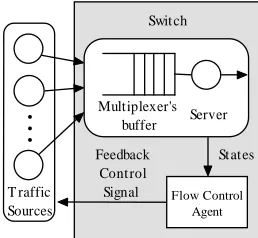
The architecture of the proposed GFQC is shown in Figure 1. In high-speed networks, GFQC in bottleneck node acts as a flow control agent with flow control ability. The inputs of GFQC are state variables S in high-speed networks composed of the current queue length q , the current change rate of queue length L q , &L and the current change rate of source sending rate u . &
The output of GFQC is the feedback signal a to the traffic sources, which is the ratio of the sending rate. It determines the sending rate u of traffic sources. The learning agent and the network environment interact continually in the learning process. At the beginning of each time step of learning, the controller senses the states for the network and gets the reward signal. Then it selects an action to make decision on which ratio the sources should use to determine the source sending rate. The determined sending rate can reduce the PLR and increase the link utilization. After the sources take the determined rate to send the traffic, the network changes its state and gives a new reward to the controller. Then the next step of learning begins.
2.2.
Fuzzy Q-Learning Flow Controller
Q-learning learns utility values (Q-values) of state and action pairs. During the learning process, learning agent uses its experience to improve its estimate by blending new information into its prior experience.
Swit ch
Server Multiplexer's buffer
Flow Control Agent
St at es
M
Feedback Cont rol Signal T raffic
[image:2.595.324.539.321.406.2]Sources
Figure 1. Architecture of the proposed GFQC.
In general form, Q-learning algorithm is defined by a tuple <S A r p, , , >, where S is the set of discrete state space of high-speed networks; A is the discrete action space, which is the feedback signal to traffic sources;
:S A× →R
r is the reward of the agent; p:S A× →∆( )s
is the transition probability map, where ∆ ∈( )s [0,1] is the set of probability distributions over state space S.
Q-learning provides us with a simple updating procedure, in which the learning agent starts with arbitrary initial values of Q s a for all ( , ) s∈S, a∈A, and updates the Q-values as
(
) (
) (
)
(
)
1 , 1 , max 1,
t t t t t t t t t
a
Q+ s a = −α Q s a +αr +β Q s+ a
(1) where α is the learning rate and β ∈[0,1) is the discount rate [9].
It is vital to choose an appropriate r in Q-learning [10]. In this paper, based on the requirement and experience of the buffer, r is defined as
0 1.1 or 0.9
1.1
1.1 0.1
0.9
0.9 0.1
1
L LT L LT
LT L
LT L LT
LT
L LT
LT L LT
LT
L LT
q q q q
q q
q q q
q r
q q
q q q
q
q q
≥ ≤
−
< <
=
−
< <
=
(2)
where qLT is the set value of queue length in the buffer. Refer to (2), if the value of q is less than 0.9L qLT or more than 1.1qLT, r=0, the control result should be considered bad. If the value of q is equal to L q , L
1
=
r , it can be thought that the control result is good. Otherwise, r is in the range (0,1), the larger r is, the better control affects.
In Q-learning based control, the usual approach of storing the Q-values in a look-up table is impractical in the case of a large state space in high-speed networks. Furthermore, it is unlikely to visit each state in a reasonable time. Fuzzy Q-learning is an adaptation of Q-learning for fuzzy inference system, where both the actions and Q-values are inferred from fuzzy rules [11].
In high-speed networks, FIS relies on three parameters S( ,& , )&
L L
q q u to generate a selected action a . For an input state s={ ,& , }&
L L
q q u , we find the activate
value of each rule i:ω( )s i
R . Each rule has m possible discrete control actions A={ ,a a1 2,L,am}, and a parameter called q value associated with each control action. The state associates to each action in R , a quality i
with respect to the task. In FQL, one builds an FIS with competing actions for each rule i∈N designated as
1 2 3
: If is and is and is then is with
i i i i
L L
i i
j j
R q L q L u L
a a q
& &
(3)
[image:2.595.106.235.616.735.2]i s
L =linguistic term (fuzzy label) of input variable s in s
rule R , its membership function is denoted by i µ i s L .
The q values in (3) are calculated according to total
accumulated rewards and rules’ activate values.
The functional blocks of FIS are a fuzzifier, a defuzzifier, and an inference engine containing a fuzzy rule base [12]. The fuzzifier performs the function of fuzzification that translates the value of each input linguistic variable into fuzzy linguistic terms. These fuzzy linguistic terms are defined in a term set F( )S and are characterized by a set of membership function µ( )S . The defuzzier describes an output linguistic variable of selected action a by a term set F a , characterized by ( ) a set of membership functions µ( )a , and adopts a
defuzzification strategy to convert the linguistic terms of ( )
F a into a nonfuzzy value representing selected action a .
The term set should be determined at an approximate level of granularity to describe the values of linguistic variables. The term set for q is defined as L F q( L)=
{Low L ( ), Medium M High H( ), ( )}, which is used to
describe the degree of queue length as “Low”, “Medium”, or “High”. The term set for &
L
q is defined as
(&L)={ ( ), ( )}
F q Decrease D Increase I , which describes
the change rate of queue length as “Decrease” or “Increase”. The term set for u is defined as & F u( )& =
{Negative N Positive P( ), ( )}, which describes the change
rate of source sending rate as “Negative” or “Positive”. On the other hand, in order to provide a precise graded feedback signal in various states, the term for feedback signal is defined as F a( )={Higher HE ( ), High H( ),
( ), ( ), ( )}
Normal N Low L Lower LE . The membership
functions (MFs) are shown in Figure 2.
In each rule R , the learning agent (controller) can i choose one action i
j
a from the action set A=
1 2
{ ,a a ,L,am}. The inferred global continuous action a t
at state s is calculated as
( )
( )
1 1 N i i t j i t N i t i a a ω ω = = =∑
∑
s s (4) 1 1 1 L q& u& L q a ( )L qL
µ µM( )qL µH( )qL µD( )q&L µI( )q&L
( ) P u µ & ( ) N u µ & HE µ H µ N µ L µ (a) (b) (c) (d) 0
LE L0 N0 H0 HE0 LE
µ
1
a
MLbMaHa1Lb1MbHaMb1Hb
a
L −Da−Db−Ia1 Db1Ia Ib
a
N
− −Nb−Pa1 Nb1 Pa Pb
Figure 2. MFs of term set (a) F q( L), (b) F q(&L), (c) F u( )& , and (d) F a( ).
where aij is the action selected in rule i
R using a Metropolis criterion based exploration/exploitation policy in [8].
Following fuzzy inference, the Q-value for the inferred action at is calculated as
(
)
( )
( )
1 1 , ω ω = = =∑
∑
s s s N i i t j it t N
i t i
q
Q a (5)
Under action a( )st , the system undergoes transition
1
+
→
st r st where r is the reward received by the controller. This information is used to calculate temporal difference (TD) approximation error as
(
1) (
)
max , ,
β +
∆ = + ⋅ st − st t
a
Q r Q a Q a (6)
The change of q value can be found by
( )
( )
1 ω ω = ∆ = ∆ ⋅∑
s s i t i j N i t iq Q (7)
We can rewrite the learning rule (1) of q parameter values as
α ← + ⋅∆
i i i
j j j
q q q (8)
2.3.
The Genetic Operator Based Flow Controller
In this section we develop the fuzzy Q-learning controller by genetic operators. The consequent parts of fuzzy rules need to compete for survival within a niche. In this case, each rule in FIS maintains a q value, but it is no longer an estimation of accumulated rewards. The max operator in standard fuzzy Q-learning is not used since the rules that have maximum q value no longer represent rules with the best rewards. Because it is not suitable to use the q values as the fitness values in the learning, we employ their changes ∆q as the fitness
values. In this paper the fuzzy rule in (3) can be rewritten as follows:
1 2 3
: If is and is and is then is with and
i i i i
L L
i i i
j j j
R q L q L u L
a a q ∆q
& &
(9)
The fitness value for a rule is an inverse measure of
∆q . By using the fitness value calculation in [13], a
predicted rule accuracy κ at time step t is defined as
( 0)
0 otherwise η κ η − ∆ −∆
∆ > ∆
= t q q t t
e q q
(10)
The accuracy falls off exponentially for ∆ > ∆qt q0.
0
∆q is an initial value. The predicted accuracy in (10) can be used to adjust rule’s fitness value ft using the standard Widrow-Hoff delta rule
(
)
χ κ
= + −
t t t t
f f f (11)
[image:3.595.69.277.513.722.2]The niche genetic operators can prevent the population from the premature convergence or the genetic drift resulting from the selection operator. The niche genetic operators maintain population diversity and promote the formation of sub-population in the neighbourhood of local optimal solutions. In fuzzy Q-learning, the fitness sharing is implicitly implemented by assigning fitness values to the activated rules based on their contributions. The fuzzy rule antecedent constitutes an evolving niche or sub-population where the fuzzy rules with the same antecedent share similar environment states. The rule consequences or actions need to compete for survival within a niche, while the rules from different niches co-operate to generate the output.
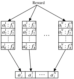
In the definition of a fuzzy rule in (9), a fuzzy rule can be defined as a sub-population and the rule actions are encoded as individuals in sub-population. If there are N
rules in fuzzy Q-learning, there will be N
sub-population. As shown in Figure 3, in each learning step, the reward from the environment is apportioned to the rules that are activated in the previous step. The rule’s fitness values are accordingly updated in the form of (11). There is a winner action in each sub-population and the winner actions from all sub-population are formed the consequent parts of fuzzy rules. The selection for the winners in sub-population is implemented by the niche genetic operator. The niche genetic operator uses two operators to select the actions:
Reproduce operator: individuals in each sub- population are selected as winners in terms of their fitness values. The roulette wheel selection is used.
Mutation operator: the mutation is taken for each sub-population with a mutation probability. The operator chooses an individual from sub-population randomly to replace a winner in the sub-population.
In the learning process, the network environment provides current states and rewards to the learning agent. The learning agent produces actions to perform in the network. The learning agent includes a performance component, a reinforcement component, and a discovery component.
The performance component reads states from network environment, calculates activation degrees of fuzzy rules, and generates an action. The action is then
1 1
1: 1
a f
1 1
2: 2
a f
1 1
: K K
a f
M
2 2
1: 1
a f
2 2
2: 2
a f
2 2
: K K
a f
M
L
1 : 1
N N
a f
2 : 2
N N
a f
: N N K K
a f
M
1 j
a 2
j
a
L
aNj [image:4.595.106.236.602.740.2]Reward
Figure 3. Learning mechanism of genetic operator.
executed by the traffic sources. The network moves into next state and receives evaluating reward from the network environment for its action.
The discovery component plays an action selection role. Two genetic operators are used to implement the selection. Finally, a set of rule actions is selected for the performance component.
The reinforcement component serves to assign the reward to the individual rules that are activated by current state.
3. Simulation and Comparison
The simulation model of high-speed network, as shown in Figure 4, is composed of two switches, Sw1 with a control agent and Sw2 with no controller are cascaded. The constant output link L is 80Mbps. The sending rates of the sources are regulated by the flow controllers individually.
In the simulation, we assume that all packets are with a fixed length of 1000bytes, and adopt a finite buffer length of 20packets in the node. On the other hand, the offered loading of the simulation varies between 0.6 and 1.2 corresponding to the systems’ dynamics; therefore, higher loading results in heavier traffic and vice versa. For the link of 80Mbps, the theoretical throughput is 62.5K packets.
From the knowledge of evaluating system performance, the parameters of the membership functions for input linguistic variables in FIS are selected as follows. For
( )
µL qL , µM(qL) , and µH(qL) , La =0 , Lb =6 ,
1 =10
b
L , Ma1 =2 , Ma =8 , Mb =12 , Mb1 =20 ,
1 =9
a
H , Ha =14 , Hb =20 , and Hb1 =20 ; for
( )
µ &
D qL and µI(q&L) , Da =4 , Db =Db1 =2 ,
1 = =2
a a
I I , and Ib =4 ; for µN( )u& and µP( )u& , 0.8
=
a
N , Nb =0.4, Nb1 =0.2, Pa1 =0.2, Pa =0.4,
and Pb =0.8. Also, the parameters of the membership functions for output linguistic variables are given by
0 =0.2
LE , L0 =0.4 , N0 =0.6 , H0 =0.8 , and
0 =1
HE .
The fuzzy rule base is an action knowledge base, characterized by a set of linguistic statements in the form of “if-then” rules that describe the fuzzy logic relationship between the input variables and selected action. After the leaning process, the inference rules in fuzzy rule base under various system states are shown in Table I. According to fuzzy set theory, the fuzzy rule base forms a fuzzy set with dimensions 3×2×2=12. For example, rule
Sw1
control agent
Sw2
Sn Dn
D1 L
L:80Mbps S1
[image:4.595.339.507.666.728.2]M
M
1 can be linguistically started as “if the queue length is low, the queue length change rate is decreased, and the sending rate change rate is negative, then the feedback signal is Higher.”
In the simulation, four schemes of flow control agent, AIMD, standard reinforcement learning-based neural flow controller (RLNC), Metropolis criterion based Q- learning flow controller (MQLC), and the proposed GFQC are implemented individually in high-speed network. The first scheme AIMD increases its sending rate by a fixed increment (0.11) if the queue length is less than the predefined threshold; otherwise the sending rate is decreased by a multiple of 0.8 of the previous sending rate to avoid congestion [14]. Finally, for the other schemes, the sending rate is controlled by the feedback control signal a periodically. The controlled t sending rate is defined by the equation
= t t
u a FL (12)
where at∈[0.2,1.0] is the feedback signal by the
flow controller, F is a relative value in the ratio of source offered load to the available output bit rate, L denotes the outgoing rate of link, and ut∈[0.2⋅FL FL, ]
is the controlled sending rate at sample time t.
In simulation four measures, throughput, PLR, buffer utilization, and packets’ mean delay, are used as the performance indices. The throughput is the amount of received packets at specified nodes (switches) without retransmission. The status of the input multiplexer’s buffer in node reflects the degree of congestion resulting in possible packet losses. For simplicity, packets’ mean delay only takes into consideration the processing time at node plus the time needed to transmit packets.
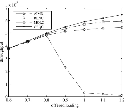
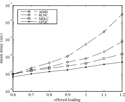
[image:5.595.319.529.78.261.2]The performance comparison of throughput, PLR, buffer utilization, and mean delay controlled by four different kinds of agents individually are shown in Figure 5-8. The throughput for AIMD method decrease seriously at loading of 0.9. Conversely, the GFQC proposed remain a higher throughput even though the offered loading is over 1.0, and can decrease the PLR enormously with high throughput and low mean delay. The GFQC has a better performance over RLNC and MQLC in PLR, buffer utilization, and mean delay. It demonstrates once again that GFQC possesses the ability to predict the network behavior in advance.
Table 1. Rule table of FIS.
Rule qL q&L u& a Rule qL q&L u& a
1 L D N HE 7 M I N N
2 L D P H 8 M I P LE
3 L I N N 9 H D N L
4 L I P N 10 H D P LE
5 M D N H 11 H I N L
6 M D P L 12 H I P LE
0.6 0.7 0.8 0.9 1 1.1 1.2
0 1 2 3 4 5 6 7x 10
5
offered loading
th
ro
u
g
h
p
u
t
AIMD RLNC MQLC GFQC
Figure 5. Throughput versus various offered loading.
0.6 0.7 0.8 0.9 1 1.1 1.2
10-8 10-6 10-4 10-2 100
offered loading
p
a
c
k
e
t
lo
ss
r
a
ti
o
AIMD RLNC MQLC GFQC
Figure 6. PLR versus various offered loading.
0.6 0.7 0.8 0.9 1 1.1 1.2
0 5 10 15 20
offered loading
m
e
a
n
b
u
ff
e
r
(p
a
c
k
e
t)
AIMD RLNC MQLC GFQC
[image:5.595.312.533.312.494.2] [image:5.595.310.538.537.727.2]0.6 0.7 0.8 0.9 1 1.1 1.2
10-6
10-5
10-4
10-3
10-2
10-1
offered loading
m
e
a
n
d
e
la
y
(
se
c
)
[image:6.595.66.278.79.252.2]AIMD RLNC MQLC GFQC
Figure 8. Mean delay versus various offered loading.
4.
Conclusions
In the flow control of high-speed networks, the reactive scheme AIMD could not accurately respond to a time-varying environment due to the lack of prediction capability. The fuzzy Q-learning flow controller has good performance when the state space of high-speed network is large and continuous. The genetic operator is introduced to obtain the consequent parts of fuzzy rules. Through a proper training process, the proposed GFQC can respond to the networks’ dynamics and learn empirically without prior information on the environmental dynamics. The sending rate of traffic sources can be determined by the well-trained flow control agent. Simulation results have shown that the proposed controller can increase the utilization of the buffer and decrease the PLR simultaneously. Therefore, the GFQC proposed not only guarantees low PLR for the existing links, but also achieves high system utilization.
5.
References
[1] R. G. Cheng, C. J. Chang, and L. F. Lin, “A QoS- provisioning neural fuzzy connection admission con- troller for multimedia high-speed networks,” IEEE/ ACM Transactions on Networking, Vol. 7, No. 1, pp. 111-121, 1999.
[2] M. Lestas, A. Pitsillides, P. Ioannou, and G. Hadjipollas, “Adaptive congestion protocol: A congestion control protocol with learning capability,” Computer Networks: The International Journal of Computer and Telecommunications
Networking, Vol. 51, No. 13. pp. 3773-3798, September 2007.
[3] R. S. Sutton and A. G. Barto, “Reinforcement learning an introduction,” Cambridge, MA: MIT Press, 1998. [4] A. Chatovich, S. Okug, and G. Dundar, “Hierarchical
neuro-fuzzy call admission controller for ATM networks,” Computer Communications, Vol. 24, No. 11, pp. 1031- 1044, June 2001.
[5] M. C. Hsiao, S. W. Tan, K. S. Hwang, and C. S. Wu, “A reinforcement learning approach to congestion control of high-speed multimedia networks,” Cybernetics and Systems, Vol. 36, No. 2, pp. 181-202, January 2005.
[6] K. S. Hwang, S. W. Tan, M. C. Hsiao, and C. S. Wu, “Cooperative multiagent congestion control for high- speed networks,” IEEE Transactions on System, Man, and Cybernetics-Part B: Cybernetics, Vol. 35, No. 2, pp. 255-268, April 2005.
[7] X. Li, X. J. Shen, Y. W. Jing, and S. Y. Zhang, “Simulated annealing-reinforcement learning algorithm for ABR traffic control of ATM networks,” in Proceedings of the 46th IEEE Conference on Decision and Control, New Orleans, LA, USA, pp. 5716-5721, December 2007.
[8] X. Li, Y. W. Jing, G. M. Dimirovski, and S. Y. Zhang, “Metropolis criterion based Q-learning flow control for high-speed networks,” in 17th International Federation of Automatic Control (IFAC) World Congress, Seoul, Korea, pp. 11995-12000, July 2008.
[9] C. J. C. H. Watkins, and P. Dayan, “Q-learning,” Machine Learning, Vol. 8, No. 3, pp. 279-292, May 1992.
[10] M. L. Littman, “Value-function reinforcement learning in Markov games,” Journal of Cognitive System Research, Vol. 2, No.1, pp. 55-66, 2001.
[11] D. B. Gu, and E. F. Yang, “A policy gradient reinforce- ment learning algorithm with fuzzy function approxi- mation,” in Proceedings of the 2004 IEEE International Conference on Robotics and Biomimetics, Shenyang, China, pp. 934-940, August 2004.
[12] Y. Zhou, M. J. Er, and Y. Wen, “A hybrid approach for automatic generation of fuzzy inference systems without supervised learning,” in Proceedings of the 2007 American Control Conference, New York City, USA, pp. 3371-3376, July 2007.
[13] S. W. Wilson, “Classifier fitness based on accuracy,” Evolutionary Computation, Vol. 3, No. 2, pp. 145-179, 1994.