An Adaptive Differential Evolution Algorithm to Solve Constrained Optimization Problems in Engineering Design

Engineering, 2010, 2, 65-77

doi:10.4236/eng.2010.21009 lished Online January 2010 (http://www.SciRP.org/journal/eng/).

65 Pub

An Adaptive Differential Evolution Algorithm to Solve

Constrained Optimization Problems in Engineering Design

Youyun AO1_{, Hongqin CHI}2

1_{School of Computer and Information, Anqing Teachers College, Anqing, China} 2_{Department of Computer, Shanghai Normal University, Shanghai, China}

Email: [email protected], [email protected]

Received July 28, 2009; revised August 23, 2009; accepted August 28, 2009

Abstract

Differential evolution (DE) algorithm has been shown to be a simple and efficient evolutionary algorithm for global optimization over continuous spaces, and has been widely used in both benchmark test functions and real-world applications. This paper introduces a novel mutation operator, without using the scaling factor F, a conventional control parameter, and this mutation can generate multiple trial vectors by incorporating dif-ferent weighted values at each generation, which can make the best of the selected multiple parents to im-prove the probability of generating a better offspring. In addition, in order to enhance the capacity of adapta-tion, a new and adaptive control parameter, i.e. the crossover rate CR, is presented and when one variable is beyond its boundary, a repair rule is also applied in this paper. The proposed algorithm ADE is validated on several constrained engineering design optimization problems reported in the specialized literature. Com-pared with respect to algorithms representative of the state-of-the-art in the area, the experimental results show that ADE can obtain good solutions on a test set of constrained optimization problems in engineering design.

Keywords:

Differential Evolution, Constrained Optimization, Engineering Design, Evolutionary Algorithm,

1. Introduction

Many real-world optimization problems involve multiple constraints which the optimal solution must satisfy. Usu-ally, these problems are also called constrained optimiza-tion problems or nonlinear programming problems. En-gineering design optimization problems are constrained optimization problems in engineering design. Like a con-strained optimization problem, an engineering design optimization problem can be generally defined as follows [1–4]:

Minimize f(x), x[x1,x2,...,xn]n



Subject to gj(x)0,j1,2,...,q 

(1) m

q q j x

h_j()0,  1, 2,..., where LixiUi,i1,2,...,D

Here, is the number of the decision or parameter variables (that is,

n

x is a vector of size ), the variable varies in the range . The function

D ith

i

x [L_i,U_i]

) (x

f  is the objective function, g_j(x) is the ine-quality constraint and

th j )

(x

h_j  is the equality con-straint. The decision or search space is written as

, the feasible space expressed as th

S

0 j

) ( ;





S

{



D i 1[Li,Ui]

(

| )0, 1,2,...,  ,  1,



 x S gj x j qhj x j q

F  

} ,...,m 2

q is one subset of the decision space (ob-viously, ) which satisfies the equality and ine-quality constraints.

S S

F

optimization problems. Zhang et al. [8] proposed a dif-ferential evolution with dynamic stochastic selection to constrained optimization problems and constrained en-gineering design optimization problems. Akhtar et al. [9] proposed a socio-behavioural simulation model for en-gineering design optimization. He and Wang [10] pro-posed an effective co-evolutionary particle swarm opti-mization for constrained engineering design problems. Wang and Yin [11] proposed a ranking selection-based particle swarm optimizer for engineering design optimi-zation problems. Differential evolution (DE) [12,13], a relatively new evolutionary technique, has been demon-strated to be simple and powerful and has been widely applied to both benchmark test functions and real-world applications [14]. This paper introduces an adaptive dif-ferential evolution (ADE) algorithm to solve engineering design optimization problems efficiently.

The remainder of this paper is organized as follows. Section 2 briefly introduces the basic idea of DE. Section 3 describes in detail the proposed algorithm ADE. Sec-tion 4 presents the experimental setup adopted and pro-vides an analysis of the results obtained from our em-pirical study. Finally, our conclusions and some possible paths for future research are provided in Section 5.

2. The Basic DE Algorithm

Let’s suppose that [ _,1, _,2,..., t_, ] D i t i t i t

i x x x

x 



are solutions at generation t, Pt {x₁t,x₂t,...,x_Nt} is the population, where denotes the dimension of solution space, is the population size. In DE, the child population

D N

1  t

P is generated through the following operators [12,15]:

1) Mutation Operator: For each xit



in parent popu-lation, the mutant vector v_it1 is generated according to the following equation:

)

( _{2 3}

1 1 t r t r t r t

i x F x x

v      ₍₂₎

where are randomly chosen and

mutually different, the scaling factor i

N r

r

r₁, ₂, ₃{1,2,..., }\

F controls

ampli-fication of the differential variation

(

)

x





x



2) Crossover Operator: For each individual x_it, a trial vector t1

i

u is generated by the following equation:

         otherwise , ]) , 1 [ || ( if , , 1 , 1 , t j i t j i t j i _x D rand j CR rand v

u (3)

where is a uniform random number distributed be- tween 0 and 1, is a randomly selected index from the set { , the crossover rate

rand ] , 1 [ D rand } ,..., 2 ,

1 D CR[0,1]

controls the diversity of the population.

3) Selection Operator: The child individual x_it1 is

selected from each pair of xit



and uit1



by using gree- dy selection criterion:

        , )) ) ( if , 1 1 1 t i t t i t i x u

x   (

t i

x f otherwise

(u_i

f  



 ₍₄₎

where the function is the objective function and the condition

f f( ) )

(uit 1 xit

f    _{means the individual} t1 i

u is better than xit



.

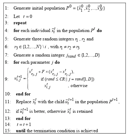
Therefore, the conventional DE algorithm based on scheme DE/rand/1/bin is described in Figure 1 [15].

3. The Proposed Algorithm ADE

3.1. Generating Initial Population Using Orthogonal Design Method

Usually, the initial population P0{x₁0,x₂0,...,x_N0}

( rj U

D

of evolutionary algorithms is randomly generated as follows:

) :

, j D xi0 Lj j Lj

N

i    

 _,j  (5)

where is the population size, is the number of variables, is a random number between 0 and 1, the

variable of N

j

r

th

j xi0



is written as , which is initial-ized in the range . In order to improve the search efficiency, this paper employs orthogonal design method to generate the initial population, which can make some points closer to the global optimal point and improve the diversity of solutions. The orthogonal design method is described as follows [16]:

0 ,j i x ,..., , 2 1 x ] j x , jU L [

For any given individual [x xD]



, the ith

1: Generate initial populationP0{x₁0,x₂0,...,x_N0}

2: Let t0 3: repeat

4: for each individualx_itin the populationPtdo

2 r ,..., 2 , 1 D

5: Generate three random integersr₁, and 6: r₃{1,2,...,N}\i, withr₁r₂r₃

j

7: Generate a random integer _rand{ } 8: for each parameterjdo

9:             otherwise ( if ), ( , , , 1 , 1 3 t j i t j r t j r t j i x rand rand x F x u  , || , 2 t j r j CR x ]) , 1 [ D

10: end for

11: Replacex_itwith the childu_it1in the populationPt1,

12: ifu_it1is better, otherwisex_itis retained 13: end for

14: tt1

15: until the termination condition is achieved

Figure 1. Pseudocode of differential evolution based on scheme DE/rand/1/bin.

Y. Y. AO ET AL. 67 decision variable varies in the range . Here,

each is regarded as one factor of orthogonal design. Suppose that each factor holds levels, namely, quan-tize the domain into Q levels

i

x

[L_i

] , [L_i U_i

i

x

Q ]

,U_i   ,...,_Q

j i,



, ₂

1 .

The level of the factor is written as , which is defined as follows:

th

j ith

             _ Q j U Q j j L j L a i Q L U i i j

i i i

, 1 2 , ) )( 1 ( 1 , 1

, (6)

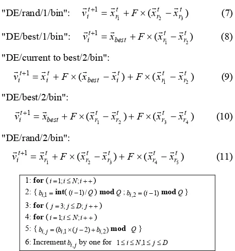
And then, we create the orthogonal array M

with factors and Q levels, where is the number of level combinations. The procedure of con-structing one orthogonal array is de- scribed in Figure 2.

D N j i

b ) _

( , D N

D N j i b _ ( _, ) M

Therefore, the initial population is generated by using the orthogonal array , where the variable of individual

D N j i x P0( 0_, ) _

N j i

b M ( _, ) _

0 i

x

D th

j  is 0



,j i

x

a

3.2. Multi-Parent Mutation Scheme

According to the different variants of mutation, there are several different DE schemes often used, which are for-mulated as follows [12]:

"DE/rand/1/bin": v_it1 x_rt₁ F(x_rt₂ x_rt₃) (7)

"DE/best/1/bin": 1 ( ₁ t₂) r t r best

t

i x F x x

v        ₍₈₎

"DE/current to best/2/bin":

) (

)

( _{1 2}

1 t r t r t i best t i t

i x F x x F x x

v            ₍₉₎

"DE/best/2/bin":

) (

)

( _{1 2 3 4}

1 t r t r t r t r best t

i x F x x F x x

v            ₍₁₀₎

"DE/rand/2/bin":

) (

)

( _{2 3 4 5}

1 1 t r t r t r t r t r t

i x F x x F x x

v            ₍₁₁₎

1: for (i1;iN;i)

2: {b_i,1int((i1)/Q) modQ;b_i,2(i1)modQ} 3: for (j3;jD;j)

4: for (i1;iN;i)

5: {bi,j(bi,1(j2)bi,2)mod Q} 6: Incrementb_i,_jby one for 1iN,1jD

Figure 2. Procedure of constructing one orthogonal array

D N i j)

(b

M  .

best

x is the best individual of the current popula-where

tion. Usually, based on both the control parameter F and the selected multiple parents, using these DE schemes can only generate a vector after a single mutation. Tsutsui et al. [17] proposed a multi-parent recombination with simplex crossover in real coded genetic algorithms to utilize the selected multiple parents and improve the di-versity of offspring. Inspired by multi-parent recombina-tion with simplex crossover, this paper proposes a novel multi-parent mutation in differential evolution. The multi- parent mutation is described in the following.

For each individual xit



from the population Pt with population size N , i1,2,...,N . A perturbed ector

1  t i v v 

is generated ccor following formula:

K _{ }

 

a ding to the



i x w xk xk v

1

1 _{( )}

1 (12)

where r₁,r₂,...,r_K{1,2,...,N}\i, K r d andomly chosen integers t r t r x

x_{K1 1}

are mutually different, an  _   . The weighted valuew_kis defined as follows:

) , 1 ( K dn 

 ran ,w/sum() (13) where randn(1,K) is a 1-by-Kmatrix with normally distributed random numbers, su () is used for calcu-lating the sum of all compon he vector 

m nts

e of t , and

] ,..., ,

[w1 w2 wK

w .

vary

According to the ingw, repeat Formulas (13) and (12) forKtimes,Knew vectors v_it1{1}, v_it1{2}, ...,

} { 1 _K

vit



are gen ated from theer seKsele ents. n

cted par And the K vectorsx_it1{1}, x_it1{2},..., x_it1{K} are

created by ossover and tr t

de-scribed in Subsections 3.3-3.5 respectively. Finally, an offspring individual t1

i

x

cr , repair cons ain handling



of the (t1)th generation population Pt1 is ob d by selecting the best indi-vidual from these Koffspring and their common parenttaine

t i

x .

.3. Adaptive Crossover Rate

rate is a constant

3 CR

conventional DE, the crossover CR In

value between 0 and 1. This paper prop an adaptive crossover rate CR, which is defined as follows:

oses

) )^ ( exp(

0 a b

CR _{  T}t



CR (14)

where the initial crossover rate is and usually is set to 0.8 or 0.85

0

CR ,

a constant value t is the current

tion number and T is the max generation number, b is a shape parameter determ ing the degree of de-pendency on the g eration number, a and b are po- s ive constants, usually a is set to 2, b is set to 2 or 3. At the early stage, DE uses a bigger crossover ate CR to preserve the diversity o solutions and revent prema-ture; at the later stage, DE employs a smaller crossover rate CR to enhance the local search and prevent the better solutions found from being destroyed.

3.4. Repair Method

imal in

more of t w

en it

e

r

variables in t f

r

p

After crossover, if one o he he

n vector uit1



are beyond their bound es, e vio-ari th lated variable value u_it_,_j1 is either reflected back from the violated b dary r set to the corresponding bound-ary value using the repair rule as follows [18,19]:

oun o             1 , t j i

e p num zation p        _ ) ( ) 3 / 1 ( if , 1 , 1 , j t j i t j i j L u p u L    ( j e e                ( ) 3 / 2 2 2 3 , ) ( ) 3 / ( 2 ( ) 3 / 2 2 ) ( 2 3 / ,2 , 1 , , j j t j i j t j i t i j j j j t i j U u U U u p U u p u U L u L L u p L u

er uniform y distributed

ran-ber in g

g chni of

olv constr e

m thod ha

  ) ) 1 1 j j ain to     ) 3 / ) 3 / 1 , 1 , t j i t j i u U u l qu ing on m  ( if / 1 ( if 1 ( if 1 ( if p p

e[0,

n    , if , , 1 , 1 , 1 , t j i j t j i

is a probability and the ran Feasibility-Based Rule ) (15) d opti-ndle wh dom In e i ] 1 .

3.5. Constraint Handli Te

volutionary algorithms for s roblems, the most com m

constraints is to use penalty functions. In general, the constraint violation function of one individual x is transformed by m equality and inequality constraints as follows [4]:



 q m

j j w x

G()  



 q j

j

j x w x

1 1 ) ) ( max( ( max  re the  |  

)) hj

g , 0 ( nt |, 0

whe expone  is usually set to 1 or 2,  is a tolerance allowed (a very small value) for the equality constraints and the c fficient w_j is greater than zero. If x

oe



is a feasible solution, G(x)0 , otherwise 0

) (x 

G  . The function value G(x) shows that the degree of constraints violation of individual x.  is

d w_j is set to 1 in this study.

In this study, a simple and efficient constraint and ing technique of feasibility-based rule is intro

also a co

set to

h l duced, which is

ra

with the better

le, the one with smaller

roposed algorithm ADE

tion Problems in

use

b , which are commonly used

2: orthogonal design method,set nd let 3: repeat

4: for each individual

2 an

nstraint handling technique without using pa-meters. When two solutions are compared at a time, the following criteria are always applied [1]:

1) If one solution is feasible, and the other is infeasible, the feasible solution is preferred;

2) If both solutions are feasible, the one objective function value is preferred;

3) If both solutions are infeasib

constraint violation function value is preferred.

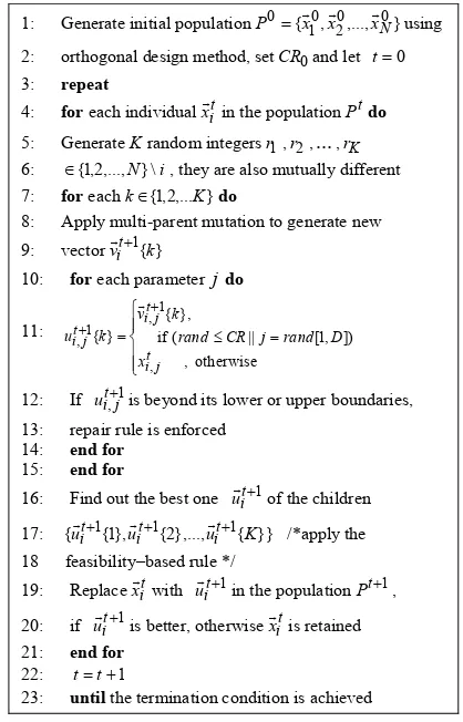
3.6. Algorithm Framework

The general framework of the p is described in Figure 3.

4. Experimental Study

4.1. Constrained Optimiza Engineering Design

In order to validate the proposed algorithm ADE, we enchmark test problems

six

1: Generate initial populationP0{x₁0,x₂0,...,x_N0}using

0

CR a t0

t i

x 

in the population do

5: Generate andom integer 6:

t

P Kr sr₁,r₂,...,r_K

i N}\ ,..., 2 , 1 {

 , they are also mutually different 7: for eachk{1,2,...K}do

8: Apply multi-parent mutation to generate new 9: vectorv_it1{k}

10: for each parameterjdo

11:            otherwise , ]) , 1 [ || ( if }, { } { , 1 , 1 , t j i t j i t j i x D rand j CR rand k v k u 

12: If is beyond its lower or upper boundaries, 13: repair rule is enforced

14: end for

15: end for

16: Find out the best one of the children

17: 1 , t j i u 1  t i u }} { },..., 2 { }, 1 {

{u_it1 u_it1 u_it1 K /*apply the 18 feasibility–based rule */

19: Replacex_itwith u_it1in the populatio ,

20: if

nPt1

1  t i

u is better, otherwise is retained 21: end for

22: t i x 1  t t

23: until the termination condition is achieved

Figure 3. The general framework of the ADE algorithm.

Y. Y. AO ET AL. 69

in th d which are de d in

the following. 1)

M

e specialized literature, an scribe

Three-bar truss design [8]: inimize f(x)(2 2x₁x₂)l

Subject to 0

2

2x₁2  x₁x₂   , 2

(_{x } x1x _{P }

g ) 2

1

0 )

( ₂ 2

2 x  P 

g

2 2x1  x1x2

x  , 0 2 1 )

(x 

g

2 1

3  

 x P 

x



where 0x11 and 0 x2 1; l100cm, ,

KN/cm2 and 2



P  2KN/cm2.

2) desi

M

Spring gn [8]:

inimize f(x) 2

2 1 3 2) (x  x x

 

Subject to 0

71785 1

)

( 1 ₄

1   

x x g , 2 3 3 x x  0 1 51 )

125 ₀₈ 2

1 ( 66 4 ) ( 2 1   x x g  2 2

1 _{  }

x x x , 4 2 3 2 1 2

x x

x 0 45 . 140

1_ 2

 x ) ( 3 x g 3 2 1  x x  , 0 1 )

(_{x } x1x2 _{ } g 5 . 1 4 

where 0.25x₁1.3, 0.05x₂2.0, and 2x₃15. 3) Pressure vessel design [9,20]:

Minimize f(x)0.6224x1x3x41.7781x2x323.1661x12x4

 3 2 1 84 . 19 x x



Subject tog1(x)x10.0193x3 0

 , 0 00954 . 0 )

( _{2 3}

2 x x  x 

g  ,

0 000 , 296 , 1 3 4 )

( 32 4 33

3 x  x x  x  

g    ,

0 240 )

( 4

4 x x  

g 

where x₁ 0.0625n₁, x₂ 0.0625n₂, 1n₁99, .

, 99

 10x3  1n2

4) W design

,

200 10x4 200

elded beam [9]:

Minimize ) 0 . 14 ( 04811 .

0 x3x4 x2



10471 . 1 )

(x x12x2

f  

Subject tog₁(x)(x)_max 0, 0 )

( )

( max

2 x  x  

g  ,

0 )

( _{1 4}

3 x x x 

g   ) 0 . 14 ( 04811 . 0 10471 . 0 )

( 12 3 4 2

4 x x x x x

g   

5.00, 0 125 . 0 ) ( ₁

5 x  x 

g  0 ) ( ) ( _max

6 x  x  

g  ,

0 ) ( )

(

7 x PP x 

g  _c

The other parameters are defined as follows:

, ) " ( 2 ) ' (

)_{ } 2_{ } 2

R x 2'"x

( 2

  ,

2x₁x₂ '

 P " , J MR   ), 2 2 x , ) 2 ( 4 2 3 1 2

2 x x

x

R  

(L P

M  

, 2 12 2 2 2 3 1 2 2 2 1        _{x x}

               

 x x x

J ( ) 6 ₂ ,

3 4x x PL x    , 4 ) ( ₃ 3 4 3 x Ex PL x    , 4 2 1 36 / 013 . 4 )

( _{2 } 3

 L 6 _   4 2 3      G E L x x EGx x Pc 

where P6000lb., L14in, _max 0.25in., , psi 600 , 13 max  , psi 106

 G

30



E 12106psi, 

, psi 0 00 , 30 max 

 0.1x₁2.0, 0.1x₂ 10.0,

, 0 . 10 1 .

0 x3  and 0.1x4 2.0. 5) Speed reducer design [8]: Minimize ) 0934 . 43 9334 . 3333

. x3214 x3 3 ( 7854 . 0 )

(x  x1x22

f  ) ( 4777 . 7 ) ( 508 .

1 x₁ x₆2x₇2  ₆3x₇2

 x

) (

7854 .

0 x4x62x5x72



Subject to ( ) 1 0

3 2 27

2 1

1   

x x x x

g  ,

0 1 5 . 397 ) ( ₂ 3 2 2 1

2   

x x x x

g  ,

0 1 93 . 1 ) ( ₄ 6 3 2 3 4

3   

x x x

x x

g  ,

0 1 93 . 1 ) ( ₄ 7 3 2 3 5

4   

x x x

x x

g  ,

0 1 0 . 110 ] 10 9 . 16 )) /( 745 [( ) ( ₃ 6 2 / 1 6 2 3 2 4

5  

   x x x x x

g  ,

0 1 0 . 85 ] 10 5 . 157 )) /( 745 [( ) ( ₃ 7 2 / 1 6 2 3 2 5

6  

   x x x x x

g  ,

0 1 40 )

( 2 3

7   

x x x

g  , ( ) 5 1 0

1 2 8 x  _xx  

g  ,

0 1 12 ) ( 2 1

9  _x  

x x

g  ,

0 1 9 . 1 5 . 1 ) ( 4 6

10 x  _x 

g  x   ,

0 1 9 . 1 1 . 1 ) ( 5 7

11  

  x x x g 

where 2.6  x1 3.6, 0.7  x2  0.8, , 3 . 8 3

.

7 ₅

,

28 7.3x₄ 

17x₃  8.3,  x 

, 9 .

3 5.0 x7  9

.

2 x6  5.5. r

6) Himmelblau’s Nonlinea Optimization Problem This problem was proposed by Himmelblau and simi-lar to problem [22] of the hmark except for the second coefficient of the first constraint. There are five design variables. The problem can be stated as fol-lows:

Minimize

Subject t [21]:

04

g benc

5 1 2

3 0.8356891 3578547

. 5 )

(x x xx

f   

141 . 40792 293239

.

37 1

 x

og₁(x)85.3344070.0056858x₂x₅

5 3 4

1 0.0022053 00026

.

0 xx  xx

 ,

0 92 

5 2 2(x) 85.334407 0.0056858x x

g   

0 0022053 .

0 00026 .

0 1 4 3 5

 xx xx , 5 2 3(x) 80.51249 0.0071317x x

g   

2_, 3 2

1 0.0021813 0029955

.

0 xx  x



0 110 

5 2 4(x) 80.51249 0.0071317x x

g   

2 3 2

1 0.0021813 0029955

.

0 xx  x

 ,

0 90 

5 3 5(x) 9.300961 0.0047026x x

g   

4 3 3

1 0.0019085 0012547

.

0 xx xx

  ,

0 25 

5 3 6(x) 9.300961 0.0047026x x

g   

4 3 3

1 0.0019085 0012547

.

0 x  xx

 x ,

0 20 

where 78x₁102, 33x₂ 45, and 27x_i 45 (i3,4,5).

Figure 5. Convergence graph for spring design.

Figure 6. Convergence graph for pressure vessel design.

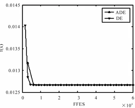
4.2. Convergence of ADE

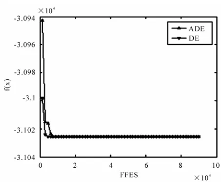
In this section, Figures 4-9 depict the convergence graphs for 6 engineering optimization problems described above respectively. From Figures 4-6, we know that ADE and DE all can be quickly convergent. In the figures, FFES is the number of fitness function evaluations.

4.3. Comparing ADE with Respect to Some S

In this experimental study, the parameter values used in ADE are set as follows: the population size

tate-of-the-Art Algorithms

50



N e level num

, the maximal generation number T 300, th ber

 

Q , the mutation parent number KD1, the Figure 4. Convergence graph for three-bar truss design.

Y. Y. AO ET AL.

Copyright © 2010 SciRes. ENGINEERING 71

Fi r

optimization problem.

initial crossover rate

gure 9. Convergence graph for Himmelblau’s nonlinea Figure 7. Convergence graph for welded beam design.

8 . 0 0 

CR , the coefficient a2, the shape parameter b3, the exponent 2. The

s equal number of fitness fu uations (FF

to

nction eval ES) i

K T

N  . The achieved sol tion at the end ofu K

T

N 

. Convergence graph for speed re gn.

Figure 8 ducer desi

FFES is easure the pe

ADE. ADE is independently run 30 times on each test problem above. The optimized objective function values (of 30 runs) arranged in ascending order and the 15th value in the list is called the median optimized function value. Experimental results are presented in Tables 1-12. And NA is the abbreviation for “Not Available”.

For three-bar truss design problem, the experimental results are given in Tables 1-2. According to Table 1, ADE and DSS-MDE [8] can obtain the approximate best and median

Table 1. Comparison of statistical results f over 30 ru

Algorithms Best Median

used to m rformance of

values, which are slightly better than those obtained by Ray

or three-bar truss design ns.

Mean Worst Std FFES

ADE 263.89584338 263.89584338 263.89584338 263.89584338 4.72e-014 45,000

DSS-MDE [8] 263.8958434 263.8958434

Ray and Liew [6] 263.8958466 263.8989

263.8958436 263.8958498 9.72e-07 15,000

263.9033 263.96975 1.26e-02 17.610

Table 2. Comparison of best solutions

Function ADE DSS-MDE [8] Ray a

found for three-bar truss design.

nd Liew [6] ECT [23] Ray and Saini [24]

1

x 0.7886751376014 0.7886751359 0.7886210370 0.78976441 0.795

2

x 0.4082482819599 0.4082482868 0

263.8958466 263.896710000 264.300

FFES 45,000 15,000 17,610 55,000 2712

.4084013340 0.40517605 0.395

) (x

Table 3. Comparison of statistical results for spring design over 30 runs.

Algorithms Best Median Mean Worst Std FFES

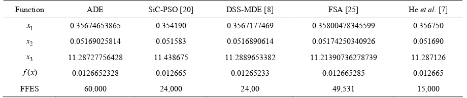
ADE 0.0126652328 0.0126652458 0.0129336018 0.02064372078 1.46e-03 60,000

SiC-PSO [20] 0.012665 NA 0.0131 NA 4.1e-04 24,000

F 0.01266 0.0126 0.012 2.

DSS-M ] 0.0 0 0. 0

Ray 0.01 0. 0.0 0.

0.0 0.0 0.01 0.0

SA [25] 5285 NA 65299 665338 2e-08 49,531

DE [8 12665233 .012665304 012669366 .012738262 1.25e-05 24,000

and Liew [6] 266924934 012922669 12922669 016717272 5.92e-04 25,167

Coello [26] 1270478 1275576 276920 1282208 NA 900,000

Table 4. Comparison of best solutions found for spring design.

SiC-PSO [20] DSS-MDE [8] FSA [25] He et al. [7]

Function ADE

1

x 0.35674653865 0.354190 0.3567177469 0.35800478345599 0.356750

2

x 0.05169025814 0.051583 0.0 0.0 26 90

1 11.2 1 9 6

0.01 8 0.0 0.012 0. 85 65

FFES 60 15,000

516890614 51742503409 0.0516

3

x 1.28727756428 11.438675 889653382 1.2139073627873 11.28712

) (x

f 2665232 12665 65233 0126652 0.0126

,000 24,000 24,00 49,531

Table 5. Comparison of stat sults for e ve r 30 r

M rst

istical re pressur ssel design ove uns.

Algorithms Best edian Mean Wo Std FFES

ADE 5885.3327736 32775885.3 85 5885.3349564 5885.3769425 8.66e-03 75,000

SiC-PSO [20] 6

R

H 2

Montes et al.[3] 6059.702 6059.702 6059.702 6059.702 1.0e-12 24,000

059.714335 NA 6092.0498 NA 12.1725 24,000

ay and Liew [6] 6171.00 NA 6335.05 NA NA 20,000

e et al.[7] 6059.714 NA 6289.929 NA 3.1e+ 30,000

and L respectiv he mean

obtained b ADE mong t rithms,

while the FFES (45 the h est. And

we also find that th s can f

ear-op-timal solutions. Fr can see that ADE can find the best value pared with respect to

DSS-MDE [ ], Ray and ], ECT [22 and

Saini [2 e best res ined by AD

iew [6] ely. T and worst values

y are the best a

,000) of ADE is alsohree algoigh ese algorithm ind the n om Table 2, we

when com Liew [6

8 ] and Ray

3]. Th ult obta E is

) (x

f  =263.8958433764684, corresponding to



x [x₁,x₂]=[0.788675137 2, 0.40824 90]

and constr

6014 8281959

aints

[g₁(x), g₂(x), g₃(x) ]

162 -0.535898 9484].

For gn prob experime results

are given in Tables 3-4. According to Table 3, ADE,

[20], FSA MDE [8 ut the

e when espect to Ray and Liew

oello [25] ue ob ADE

han ob method e mean

t value becau E can

d 29 near- utions in nd the

tio (i.e., the alue is

64372078). Tab esents the det ach best value obtained by ADE, SiC-PSO [20], DSS-MDE [8], ely. The best result

=[0, -1.46410 480516, 3751

spring desi lem, the ntal

Sic-PSO [24], DSS- ] can find o

best valu

[6] and C compared with r. The median val tained by is better t tained by other s, but th and wors s are worse, this is se that AD only fin

other is an excepoptimal soln solution 30 runs aworst v

0.020 le 4 pr ail of e

FSA [24] or He et al. [7] respectiv obtained by ADE is

) (x

f  = 0.01266523 832, ing

278

correspond to



x [x1,x2,x3]

=[0.3567 021031, 0.051689065

11.288 7073

and constraints

1785 67225,

9592785 ]

Y. Y. AO ET AL. 73 [g₁(x),g₂(x), g₃(x), g₄(x)]

=[-2.220446049250313e-016, -4.4408

) of ADE

is also the highest. etail of each

ed by 20], Ray and

l. [7] or Montes et al. [3] respectively. The best

92098500626e-016, 4.05378584839796, -0.72772872274496].

For pressure vessel design problem, the experimental results are given in Tables 5-6. According to Table 5, the best, median, mean, worst and standard deviation of val-ues obtained by ADE are the best when compared with respect to Sic-PSO [20], Ray and Liew [6], He et al. [7], and Montes et al. [3], while the FFES (75,000

Table 6 presents the d ADE, SiC-PSO [ best value obtain

Liew [6], He et a

result obtained by ADE is )

(x

f  =5885.332773616458, corresponding to

and constraints

[x₁,x₂,x₃,x₄] x



= [0.778168641375, 0.384649162628, 40.319618724099, 200]

[g₁(x),g₂(x), g₃(x), g₄(x)] =[-1.110223024625157e-016,0,0,-40].

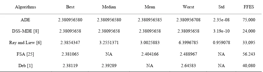
elded b gn pro the e ental

results are provided with Tables 7-8. According to Table 7, the best, median, mean, worst and standard derivation

For w eam desi blem, xperim

of values obtained by ADE are slightly worse than those obtained by DSS-MDE [8] and are better than those ob-tained by Ray and Liew [6], FSA [25] and Deb [1]. However, the FFES (75,000) of ADE is the highest. Ta-ble 8 presents the detail of each best value obtained by DSS-MDE [8], He et al. [7], FSA [25], Ray and Liew [6], and Akhtar et al. [9] respectively. The best result ob-tained by ADE is

) (x

f  = 2.3809565 8032252, corresponding to



x [x1,x2,x3,x4]

= [0.24436897580173, 6.21751971517460, .2 14 13 48 684, 0.24436897580173] and constrai

8 9 7 90 n ts

[g₁(x), g₂(x), g₃(x), g₄(x), g₅(x), g₆(x), g₇(x)] 27514e-011, -3.310560714453459e-010, -1. 78 78144 -016, -3.02295 760400, -0.

-1.27

Table 6. Comparison of best solutions

Function ADE Sic-PSO [20] R

=[-1.0913936421

387778 0 6e 458

11936897580173, -0.23424083488769, 3292582482100e-011].

found for pressure vessel design.

ay and Liew [6] He et al. [7] Montes et al. [3]

1

x 0.7781686414 0.812500 0.8125 0.8125 0.8125

2

x 0.3846491626 0.437500

40.319618724 42.098445

200 176.636595

5885.3327736 6059.714335 6171.0 60

FFES 75,000 24,000 30,000 24,000

0.4375 0.4375 0.4375

41.9768 42.098446 42.098446

182.9768 176.636052 176.636047

3

x

4 x

) (x

f 6059.7143 6059.7016

20,000

Table 7. Comparison of statistical results for welded

Algorithms Best Median Worst Std FFES

beam design over 30 runs.

Mean

ADE 2.380956580 2.380956580 2.380956585 2.3809 708 2.35e-08 75,000 56

DSS-MDE [8] 2.38095658 2.38095658 2.38095 ,000

Ray and Liew [6] 2.3854347 3.2551371

FSA [25] 2.381065 NA

Deb [1] 2.38119 2.39289

658 2.38095658 3.19e-10 24

3.0025883 6.3996785 0.959078 33,095

2.404166 2.488967 NA 56.243

NA 2.64583 NA 40,080

ions found for

Ray and Liew [6] Akhtar et al. [9]

welded beam design. Table 8. Comparison of best solut

Function ADE DSS-MDE [8] He et al. [7] FSA [25]

1

x 0.24436897580 0.2443689758 0.244369 0.24435257 0.244438276 0.2407

2

x 6.21751971517 6.2175197152 6.217520

8.2 05 8.291471 9

7580 0.2443689758 0.244369 0.2497

2.3809 8032 2.38095658 2.380957 2.381065 2.3854347 2.4426

FFES 75,000 24,000 30,000 56,243 33,095 19,259

6.2157922 6.237967234 6.4851

8.2939046 8.288576143 8.239

0.24435258 0.244566182

3

x 9147139049 8.29147139

4 0.2443

x 689

565

) (x f

Table 9. Comparison of statistical results cer desi runs.

Algorithms Mean Worst Std ES

for speed redu gn over 30

Best Median FF

ADE 2994.4710662 2994.4710662 2994.4710662 2994.4710662 1.85e-012 120,000

DSS-MDE [8] 066 2994.4 2994.471 3.58e-012 0

Ray and Liew [6] .744241 3001.7 3009.96 423 6

Monte [27] 689 2996.36 NA 8.2e-03

et al. [9] 8.08 3012 3028 NA 154

2994.471 2994.471066 71066 066 30,00

2994 3001.758264 582264 4736 4.0091 54,45

s et al. 2996.356 NA 7220 24,000

Akhtar 300 NA .12 19,

Functi ADE DSS-MDE Ray and L Mon [27] khtar et

Table 10. Comparison of best solutions found for speed reducer design.

on [8] iew [6] tes et al. A al.[9]

1

x 3.5 3.5 3.50000681 3.500010 3.506122

2

x 0.7 0.7 0.70

17 17 1 17

7.3 7.3 7.3276 7.5491

7.715319911478 7.7153199115 7.71532175 7.800027 7.859330

3.350214666096 3.3502146661 3.35026702 3.350221 3.365576

5.28665446 5.289773

2994.4710662 2994.471066 2994.744241 2996.356689 3008.08

1

000001 0.7 0.700006

3

x 7 17

4

x 0205 7.300156 26

5 x

6 x

7

x 4980 5.2866544650 5.28665450 5.286685

) (x f

FFES 20,000 30,000 54,456 24,000 18,154

T aris al res imme linear problem.

Algor ms Best ean Wor Std S

able 11. Comp on of statistic ults for h lblau’s non optimization

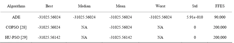
ith Median M st FFE

ADE -31025.56024 -31025.56024 -31025.56024 -31025.56024 5.91e-010 000 90,

COPSO [28] 56024 A 25.56024 NA 0 ,000

HU-PSO [29] -31025.56142 NA -31025.56142 NA 0 200,000

-31025. N -310 200

Y. Y. AO ET AL.

Copyright © 2010 SciRes. ENGINEERING 75

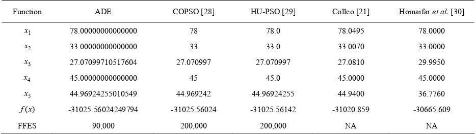
Table 12. Comparison of best solutions found for himmelblau’s nonlinear optimization problem.

Function ADE COPSO HU-[28] PSO [29] Colleo [21] Homaifar et al. [30]

1

x 78.00000000000000 78 78.0 78.0495 78.0000

2

x 33.0000 070 33.00

0709 0 29.99

0000 45.0000 45.00

.969242 9242 924255 44.9400 36.77

-31025.56024249794 -31025.56024 -31025.56142 -31020.859 -30665.609

FFES 9 NA

0000000000 33 33.0 33.0 00

3

x 27. 9710517604 27.070997 27.070997 27.081 50

4

x 45. 0000000000 45 45.0 00

5

x 44 55010549 44.96 44.96 60

) (x f

0,000 200,000 200,000 NA

F reduce gn problem mental

results ar given in Ta es 9-10. Accordi o Table 9, the best, median, mean, worst and standa erivation of values ob ained by A nd DSS-MDE [ re superior to those obtained by R Liew [6], M s et al. [27]

and Akh et al. [9 ely, wh e FFES

(120,000 of ADE is highest. Table shows the

detail of h b ned b -MDE

[8], Ray and Liew [6], Montes et al. [27] and Akhtar et

al. [9] respective ult ob E is

or speed r desi , the experi

e bl ng t

rd d

t DE a 8] a

ay and ] respectiv

onte ile th tar

) the 10

eac est value obtai y ADE, DSS

ly. The best res tained by AD )

x



x [x₁,x₂,x₃,x₄,x₅]

= [78, 33 971051760

44.96924 010549] constraints

, 27.0709 4, 45,

255 and

[g₁(x),g₂(x),g₃(x),g₄(x),g₅(x), g₆(x)] =[0, -92, -9.59476568762383, -10.40523431237617,

, 0].

m, compar espect to sev -of-the-

rithms, AD erform bett

bench-mark test problems. It is clearly shown that ADE is

fea-d effect e constrain mization

ems in enginee esign. The rea hat ADE uses multi-parent mutation to generate a better offspring, and applies self-adaptive control parameter and effective

Conclusion

d Future

rk

paper p dapti ntial ution

) algorithm constrained timizat ngi-neering Design. Firstly, ADE employs the orthogonal

method to erate the initial popul im-prove the diversity of solutions. Secondly, a multi-parent mutation scheme is developed to improve the capacity of DE. Thirdly, in order to improve the adaptive capacity of crossover

w app djusti rate

is p ted. In addi E introduc w repair

rule onstraint ing technique he

feasi-ble- rule is also when com o

solu-t me. Finally, ADE is tested on strained

engi ing design op problem om the

specialized literature. C ared with resp eral art algori e experimen lts show

highly e and ca

re-su rms of a test set of constraine timization -5

In su ed with r eral state

art algo E can p er on six

sible an ive to solv ed opti

probl ring d son is t



= 2994.471 (

f 06614

corresponding to

] = [3.5, 0.7, 17, 7.3, 7.71531991147825,

3.3 and constraints

682020,



x



[x₁,x₂,x₃, x₄,x₅,x₆,x₇

5021466609645, 5.28665446498022] repair rule etc.

[g1(x 

),g (x),g3(x) 

, 4 x) 

,g5(x) 

,

2 g ( g (x)



6 ,g7(x)

 , )

( 8 x

g  ,

5.

s an

Wo

This roposes an a ve differe evol

(ADE for op ion in E

design gen ation to

) ( 9 x

g  ,g₁₀(x),g₁₁(x)] =[-0.073915280

4991722481039787, -0.19799852, -0.904643 2714195, 7,

-0. 24 9045560

-6 509 0.70250 00000,

-2.220 031 333333 33,

-0.05132575354183, -8.881784197001252e-016]. For Himme

best, median, mean, worst and standard derivation of

valu wn in Tab -12, it is cle at

ADE, CO O [28] [29] all can d one

near-optimal solu . Ad nally,

ADE only require which is su ior to

other sev ral algo OPSO [ 00

FFES and HU-PS FES. The b result

obtained by ADE i .6613381477

44604925

39e016, 0, -3e-016, -0.58

0000 3333

lblau’s nonlinear optimization problem, the _{exploration and the convergence speed of A}

es is sho les 11 arly seen th

PS , and HU-PSO

tion after a single run

fin ditio

s 90,000 FFES, per

e rithms, such as C 28] 200,0

O [29] 200,000 F est

s )

operator, a ne roach to a ng the crossover resen

and a c

tion, AD handl

es a ne of t

based applied paring tw

ions at a ti six con

neer timization

omp

s taken fr ect to sev

state-of-the- thms, th tal resu

that ADE is competitiv n obtain good

lts in te d op

(x

f  =-3.1025.5602424979 corres

roblems in engineering design. However, there are still so

genetic algorith plied Me-ngineering, Vol. 186, No. 2, pp. 311–338,

[2] E. Mezura o es A al e ,

“Parame-ter c d

opti-miza

-putation

ontes, C. A. Coello Coello, J. Velázquez- Re s, and . Muñoz-Dávila, “Multiple trial ctors i differential evolution for e design,” Engineer-ing Optimization, Vol. 39, No. 5, pp. 567–589, 2007.

merical con- th-, No.

[5]

for mechanical design optimiz

problems,” Eng .

.

. . Luo, and X. F. Wang, “Differential lution with y m selection for constrained

optim . 178, pp.

3043

. Tai, and T. Ray, “A socio-behavioural odel for engineering design optimization Engineering Optimization, Vo 34, No. 4, pp. 3 54,

[10]

[12] R. Storn and K. Price, “Differential evolution—A simple

, 1997.

ferential evolu-tion,” Berlin: Springer-Verlag, 2005.

nina, S. C. Esquivel, and C. A. Coello Coello, “Solving engineering optimization problems with the

rained particle swarm optimizer,” Infor-2, pp. 319–326, 2008.

[21] C. A. Coello Coello, “Use of a self-adaptive penalty

evolutionary optimization,” IEEE Transactions on

al technique

ima, “Derivative-free filter p

me things to do in the future. Firstly, we will further validate ADE in the case of higher dimensions. Secondly, we also will take some measures to improve the conver-gence speed during the evolutionary process. Addition-ally, testing some initial parameters of ADE is another future work.

6. References

[1] K. Deb, “An efficient constraint handling method for ms,” Computer Methods in Ap

chanics and E 2000.

-M nt and . G. P om que-Qrtiz ontrol in differential evolution for constraine tion,” 2009 IEEE Congress on Evolutionary Com

(CEC'2009), pp. 1375–1382, 2009. [3] E. Mezura-M

ye L ve n

ngineering

[4] C. A. Coello Coello, “Theoretical and nu

straint-handling techniques used with evolutionary algo-rithms: A survey of the state of the art,” Computer Me ods in Applied Mechanics and Engineering, Vol. 191 11-12, pp. 1245–1287, 2002.

R. Landa-Becerra and C. A. Coello Coello, “Cultured differential evolution for constrained optimization,” Computer Methods in Applied Mechanics and Engineer-ing, Vol. 195, No. 33–36, pp. 4303–4322, 2006.

[6] T. Ray and K. M. Liew, “Society and civilization: An optimization algorithm based on the simulation of social behavior,” IEEE Transactions on Evolutionary Computa-tion, Vol. 7, No. 4, pp. 386–396, 2003.

[7] S. He, E. Prempain, and Q. H. Wu, “An improved particle

swarm optimizer ation proach for engineering optimization problems,” Com-_{puters in Industry, Vol. 41, No. 2, pp. 113–127, 2000.} [22] T. P. Runarsson and X. Yao, “Stochastic ranking for

con-strained ineering Optimization, Vol. 36, No. 5, pp

585–605, 2004

[8] M. Zhang, W J evo- _{Evolutionary Computation, Vol. 4, No. 3, pp. 284–294,} 2000.

[23] K. Hans Raj, R. S. Sharma, G. S. Mishra, A. Dua, and C. Patvardhan, “An evolutionary computation

d na ic stochastic

ization,” Information Sciences, Vol –3074, 2008.

[9] S. Akhtar, K

simulation m ,” f

l. 41–3

2002.

Q. He and L. Wang, “An effective co-evolutionary parti-cle swarm optimization for constrained engineering de-sign problems,” Engineering Applications of Artificial Intelligence, Vol. 20, No. 1, pp. 89–99, 2007.

[11] J. H. Wang and Z. Y. Yin, “A ranking selection-based particle swarm optimizer for engineering design optimi-zation problems,” Structural and Multidisciplinary Opti-mization, Vol. 37, No. 2, pp. 131–147, 2008.

and efficient heuristic for global optimization over con-tinuous spaces,” Journal of Global Optimization, Vol. 11, pp. 341–359

[13] K. Price, R. Storn, and J. Lampinen, “Dif tion: A practical approach to global optimiza

[14] Z. Y. Yang, K. Tang, and X. Yao, “Self-adaptive differ-ential evolution with neighborhood search,” 2008 Con-gress on Evolutionary Computation (CEC'2008), pp. 1110–1116, 2008.

[15] H. A. Abbass, R. Sarker, and C. Newton, “PDE: A Pareto-frontier differential evolution approach for mul-tiobjective optimization problems,” Proceedings of IEEE Congress on Evolutionary Computation, Vol. 2, pp. 971– 978, 2001.

[16] Y. W. Leung and Y. P. Wang, “An orthogonal genetic algorithm with quantization for global numerical optimi-zation,” IEEE Transactions on Evolutionary Computation, Vol. 5, No. 1, pp. 40–53, 2001.

[17] S. Tsutsui, M. Yamamure, and T. Higuchi, “Multi-parent recombination with simplex crossover in real coded ge-netic algorithms,” Proceedings of the Gege-netic and Evolu-tionary Computation Conference, pp. 657–664, 1999. [18] J. Brest, V. Zumer, and M. S. Maucec, “Self-adaptive

differential evolution algorithm in constrained real-pa-rameter optimization,” 2006 IEEE Congress on Evolu-tionary Computation (CEC'2006), pp. 919–926, 2006. [19] Y. Wang and Z. X. Cai, “A hybrid multi-swarm particle

swarm optimization to solve constrained optimization problems,” Frontiers of Computer Science in China, Vol. 3, No. 1, pp. 38–52, 2009.

[20] L. C. Cag simple const matica, Vol. 3

or constrained optimisation in engineering design,” Journal of the Institution of Engineers India Part Me Me-chanical Engineering Division, Vol. 86, pp. 121–128, 2005.

[24] T. Ray and P. Saini, “Engineering design optimization using a swarm with intelligent information sharing among individuals,” Engineering Optimization, Vol. 33, No. 33, pp. 735–748, 2001.

[25] A. R. Hedar and M. Fukush

simulated annealing method for constrained continuous global optimization,” Journal of Global Optimization, Vol. 35, No. 4, pp. 521–549, 2006.

Y. Y. AO ET AL.

Copyright © 2010 SciRes. ENGINEERING 77

Evolu-sity in differential

ing

ence Symposium, pp. 53–57, [26] C. A. Coello, “Self-adaptive penalties for GA- based

optimization,” Proceedings of the Congress on

tionary Computation 1999 (CEC'99), Vol. 1, pp. 573–580, 1999.

[27] E. Mezura-Montes, C. A. Coello, and J. V. Reyes, “In-creasing successful offspring and diver

and C

evolution for engineering design,” Proceedings of the Seventh International Conference on Adaptive Comput-ing in Design and Manufacture (ACDM 2006), pp. 131– 139, 2006.

[28] A. E. Muñoz Zavala, A. Hernández Aguirre, E. R. Villa Diharce, and S. Botello Rionda, “Constrained

optimiza-tion with an improved particle swarm optimizaoptimiza-tion algo-rithm,” International Journal of Intelligent Comput

ybernetics, Vol. 1, No. 3, pp. 425–453, 2008. [29] X. H. Hu, R. C. Eberhart, and Y. H. Shi, “Engineering

optimization with particle swarm,” Proceedings of the 2003 IEEE Swarm Intellig

2003.