AND COMPUTING SOLUBILITY
Rachael Elaine Skyner
A Thesis Submitted for the Degree of PhD
at the
University of St Andrews
2017
Full metadata for this item is available in
St Andrews Research Repository
at:
http://research-repository.st-andrews.ac.uk/
Please use this identifier to cite or link to this item:
http://hdl.handle.net/10023/11746
This item is protected by original copyright
Hydrate Crystal Structures,
Radial Distribution Functions,
and Computing Solubility
Rachael Elaine Skyner
This thesis is submitted in partial fulfilment for the degree of PhD
at the
University of St Andrews
For Dad, and in memory of Bill Skyner
The two greatest men I will ever know.
Abstract
Solubility prediction usually refers to prediction of the intrinsic aqueous solubility, which is the concentration of an unionised molecule in a saturated aqueous solution at thermodynamic equilibrium at a given temperature. Solubility is determined by structural and energetic components emanating from solid-phase structure and packing interactions, solute–solvent interactions, and structural reorganisation in solution. An overview of the most commonly used methods for solubility prediction is given in Chapter 1.
In this thesis, we investigate various approaches to solubility prediction and solvation model development, based on informatics and incorporation of empirical and experimental data. These are of a knowledge-based nature, and specifically incorporate information from the Cambridge Structural Database (CSD).
A common problem for solubility prediction is the computational cost associated with accurate models. This issue is usually addressed by use of machine learning and regression models, such as the General Solubility Equation (GSE). These types of models are investigated and discussed in Chapter 3, where we evaluate the reliability of the GSE for a set of structures covering a large area of chemical space. We find that molecular descriptors relating to specific atom or functional group counts in the solute molecule almost always appear in improved regression models.
Acknowledgements
First, and foremost, I would like to thank my supervisors, Dr. John Mitchell and Dr. Colin Groom. I would particularly like to thank them for the three-hour grilling that they gave me in June 2013 (otherwise known as an interview, apparently). Other than being great at extremely long interviews, they have also both been a massive support, professionally and personally, throughout my PhD. Without them, you wouldn’t have to endure reading this thesis, as the work leading to it and the actual writing of it would not have been possible. I also have to give John extra-special thanks for his incredible proof-reading skills. I’m now a full convert to the Oxford comma.
Next on the list are my long-suffering family, who call me the eternal student (rude). Thank you, Dad, for financially supporting me when I’ve spent all of my money on food or alcohol over the last 8 years, and for listening to me, and for all of the small things that seem like nothing at the time, but mean everything. Thank you, Joanne for listening to me when I moan about work, and for looking after my Dad when I’m not there. Thank you to my younger brothers and sister for not understanding a single thing I do, forcing me to find other ways of having fun when I’m visiting. Thank you to my grandma (and to my grandad, to whom this thesis is dedicated), who also doesn’t understand what I do, but constantly tells me she’s proud, and reminds me that I’m the favourite grandkid, no matter what I do.
Thank you to all of the academics and collaborators who have spent hour upon hour with me, talking crystallography, informatics, and solubility. I am sure that if it weren’t for a lot of those conversations and conference questions, the ideas presented in this work would never have popped in to my head, or developed in the way they did. Special mentions to: everyone at CCDC (thanks for the money, too!), Dr. David Palmer and Dr. Maxim Fedorov (Strathclyde), and Dr. Tasnim Munshi (Bradford/Lincoln).
Table of Contents
Introduction 1
1.1 Overview 1
1.1.1 Thermodynamics and solubility 2
1.2 Informatics – ‘Smart’ machines in solubility prediction 5
1.2.1 Molecular descriptors 5
1.2.2 Methods 6
1.2.3 The General Solubility Equation (GSE) 7
1.3 Implicit solvation – the isotropic field as a solvent representation 8
1.3.1 Continuum models for electrostatic interactions 9
1.3.2 Continuum models for non-electrostatic interactions 12
1.4 Explicit solvation models 13
1.4.1 Free energy calculations – Monte Carlo (MC) and Molecular Dynamics (MD)
simulations 14
1.4.2 Combined Quantum Mechanical/Molecular Mechanical methodologies (QM/MM) 16
1.4.3 Explicit representations of water atoms 18
1.5 Hybrid models 20
1.5.1 Correlation functions 20
Theory & Methods 23
2.1 Crystallography 23
2.1.1 Transformations of the coordinate system 24
2.1.2 Calculating interatomic distances 25
2.2 Calculating solvation free energy 26
2.2.1 Thermodynamics of solutions 26
2.2.2 RISM 28
2.2.3 Solvation free energy from RISM 30
2.3 Machine learning & cheminformatics 31
2.3.1 Molecular representation 31
2.3.2 Molecular descriptors 32
2.3.3 Descriptor selection & linear regression 35
2.3.4 Statistical measures 38
Machine Learning and Regression Models: Predicting log S 41
3.1 Introduction 41
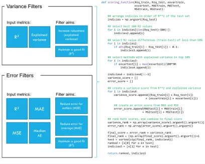
3.2 Programs developed 45
3.2.1 BruteReg: A brute force workflow to find the ‘best’ regression methods 45 3.2.2 BruteSis: A GUI enabling filters, analysis, and visualisation 49
3.3 Methods 50
3.3.1 Dataset compilation 50
3.3.4 Brute-force generation of regression models for logS 52
3.4 Results & discussion 52
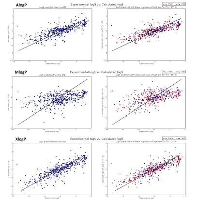
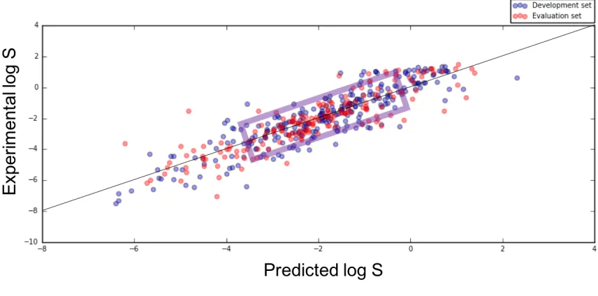
3.4.1 Assessment of the ability of the GSE to predict solubility 52 3.4.2 Extrapolating meaning from molecular descriptors 53 3.4.3 The analysis and evaluation of models calculated with BruteReg 55
Probing the Average Distribution of Water in Organic Hydrate Crystal Structures
with Radial Distribution Functions (RDFs) 61
4.1 Introduction 61
4.2 Methods 64
4.2.1 Calculation of RDFs 64
4.2.2 Deconvolution of water RDF by water motif 66
4.3 Theory 67
4.4 Results 69
4.4.1 Structure of water in hydrates 69
4.4.2 Deconvolution of water RDF by water motif 73
4.4.3 Qualitative interpretation of RDFs 75
4.5 Discussion 80
Developing Solvation Models: Application of RDFs 81
5.1 Introduction 81
5.2 Theory 84
5.2.1 Calculating the direct correlation function 84
5.2.2 HFE expressions 85
5.2.3 Relation of the partial molar volume (PMV) to g(r) 85
5.3 Methods 86
5.3.1 Dataset compilation 86
5.3.2 Solute RDF calculation 86
5.3.3 Energy expressions 87
5.3.4 Regression methods: descriptors vs. calculated terms 87
5.4 Results & discussion 87
5.4.1 HNC HFE expression 87
5.4.2 HNCB HFE expression 88
5.4.3 GF HFE expression 91
5.4.4 Regression methods: descriptors vs. calculated terms 91
Conclusions 99
6.1 Summary and conclusions 99
Introduction
Introduction
Parts of this chapter are published in; Skyner et al. Phys. Chem. Chem. Phys., 2015, 17, 6174-6191
1.1
Overview
Poor aqueous solubility is a major cause of attrition (failure) in the pharmaceutical development process and remains a vital property to quantify in the development of agrochemicals, and in the identification and quantification both of metabolites and of potential environmental contaminants. It is estimated that around 70% of pharmaceuticals in development are poorly soluble, with 40% of those currently approved also being poorly soluble1,2. Solubility is determined by structural and energetic components emanating from solid phase structure and packing interactions, in addition to relevant solute–solvent interactions and structural reorganisation in solution. This chapter focuses on the methods currently available to model the solution phase and to predict solubility for a wide range of applications, including ligand binding, molecular property prediction and molecular design3.
Accurate and timely prediction of solubility could save time and money in drug development, agrochemical development and environmental monitoring. An early-stage analysis of drug and agrochemical candidates allows organisations to focus on those molecules most likely to meet their required solubility criteria. Many models exist in this area, with differing levels of accuracy, physical interpretability, and calculation time.
Quantitative Structure Activity Relationship (QSAR) and Quantitative Structure Property Relationship (QSPR) models are very successful in this field, providing good predictive results at a reasonably low computational cost. These models, however, tend to be limited to molecules similar to those used in their training set. Moreover, these models lack a full physical interpretation, although some do allow assessments of descriptor importance that can perhaps to some extent be physically interpreted.
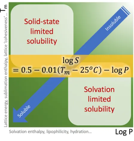
(GSE),4 taking the melting point and the base ten logarithm of the partition coefficient (log P; partition coefficient for neutral molecules in octanol and water) as empirical input.
The field has also seen the revival of old ideas as new automated data driven design protocols, such as Matched Molecular Pair Analysis (MMPA)5. MMPA allows one to acquire previously ‘unknown’ data from existing data sets by exploring how a single molecular change can impact a particular property or activity of interest. We now see large scale data mining following these kinds of protocols, consortia such as SALT MINER, and programs developed by individual companies such as GSK's BioDig.6,7
The methods mentioned thus far are often the preferred choice for industrial investigation into solubility, for example for drug-candidate screening, as pharmaceutical companies are primarily interested in a ‘rough-idea’ of how soluble a compound is. However, if a precise value or perhaps a mechanistic view of solubility is required, physics based approaches to solubility may be preferably applied. These methods vary greatly in complexity.
Classical simulations can encompass simple Molecular Dynamics (MD), studying the interactions between solute and solvent, to more complex perturbations of solutes from the solution phase to the gas phase. Recent advances have seen a new generation of polarisable force fields emerging with a greater capacity to account for changes in the electronic charge distribution. Many of these force fields utilise multipole moments, as opposed to point charges, to capture the anisotropy of the atomic charge distribution. Force fields such as Atomic Multipole Optimised Energetics for Biomolecular Applications (AMOEBA) have been used to study the solvation dynamics of ions.8 Newer, polarisable force fields, such as the Quantum Chemical Topology Force Field (QCTFF), use multipolar electrostatics calculated based on quantum chemical topology, supplemented with machine learning (Kriging) to model the system. This force field has been used to model amino acids with small water clusters.9 Some force fields can be mixed with a quantum chemical core region in mixed Quantum Mechanics–Molecular Mechanics (QM/MM) approaches.
Other common models include those representing the solvent as a continuous field with no explicit solvent coordinates. In most cases, these models come at much higher computational cost than their informatics counterparts, and often at lower accuracy. However, if such a method were feasible and accurate enough to predict solubility, it would not have a domain of applicability restricted by the molecules within a training set and would also be physically interpretable. Thus, there is a continuing search for such physical methods. These methods have proven useful for modelling or approximating the solution phase, hence their applications are diverse and widespread outside of solubility prediction.
1.1.1
Thermodynamics and solubility
Introduction
solution. Solubility and dissolution are fundamental terms describing the process of solvation, and are related by the Noyes–Whitney equation;10
!" !# =
%& '(− '
*
[1.1]
where dW/dt is the rate of dissolution, A is the solute surface area in contact with the solvent, C
is the instantaneous solute concentration in the bulk solvent, Cs is the diffusion layer solute concentration (given from the solubility of the molecule with the assumption that the diffusion layer is saturated), k is the diffusion coefficient, and L is the diffusion layer thickness.
As solubility is a thermodynamic term, it is inherently affected by factors such as temperature and pressure, as well as ionisation, solid state effects, and gaseous partial pressure for solvated gases.
pH is considered to have a significant effect on solubility, as many organic molecules can behave as weak acids or weak bases, due to ionisable basic or acidic functional groups, with polarisation of ionisable groups in solution increasing or decreasing the overall solubility. The pH of the aqueous solution in which such molecules are dissolved determines whether the molecule exists primarily in its neutral or ionised form. The charged form of a molecule is more soluble, and thus the aqueous solubility of a substance is pH-dependent.11 This dependence is described by the Henderson–Hasselbalch (HH) equations as follows;
log /01023245654= 789/
:+ log (1 + 10?@A?BC)
log /01023E2(54= 789/:+ log (1 + 10?BCA?@)
[1.2]
where Stotal is the equilibrium (thermodynamic) solubility, log S0 is the intrinsic solubility, defined as the solubility of an unionised species in a saturated solution, pKa is the negative logarithm of the ionisation constant of the molecule, and the final term on the right hand side is the solubility of the ionised form.11 The HH relationship can be utilised in the prediction of pH-dependent aqueous solubility of drugs when the pKa and log S0 values of a compound are known.12 The intrinsic solubility is a particularly important quantity as it can be used to find the pH dependent profile and estimate the pKa; it is a quantity required by industry and hence the focus of several prediction methods.13 The pH dependent profile of a drug is particularly important in pharmaceutics, as it has a direct effect on the absorption profile of a drug once it has entered the body. A basic drug-like molecule at a high pH (>2 pH units above the pKa) will be almost fully unionised with solubility at a minimum (intrinsic solubility). Protonation of the base increases as pH becomes more acidic, and solubility increases. When pH and pKa are equal, half of the solute molecules are protonated and the solubility of the drug becomes double the intrinsic solubility. According to the HH equation, this rise in solubility increases indefinitely with decreased pH, however in practice a limit is reached at the salt solubility. Two intersecting concentration curves for the base solubility and the salt solubility can be combined to give a composite curve for base solubility as a function of pH. If any one point on this curve is known (solubility and pH at which it was measured), the whole curve can be predicted providing pKa and the acid solubility factor
Intermolecular interaction strengths play an important role in the solvation of substances from the solid state. Solutes which exhibit weak intermolecular forces (i.e. are weakly bound) tend to have a higher solubility, as the energy cost of breaking up the lattice is lower. Polymorphic effects can also lead to complications in solubility prediction. A classically cited example of this is the case of the anti-HIV drug Ritonavir,15,16 in which a polymorphic shift led to a significant change in solubility, leaving the drug with a greatly reduced bio-availability. This exemplifies the consideration of solubility as a property which is dependent upon solid, solute, solvent, and solution state properties and interactions.
Two common approaches to the calculation of the Gibbs free energy of solution utilise a thermodynamic cycle approach. A first approach calculates the free energy of solution by addition of the free energy of sublimation (taking the molecule in the crystalline phase and subliming it into the gaseous phase) and free energy of solvation (taking the molecule in its gaseous phase and solvating it into aqueous solution). Examples of this approach are well cited within the literature.13,17,18 A second approach involves calculation of the free energy of solution by addition of the free energy of fusion (taking a molecule from the crystalline state to a hypothetical supercooled liquid) and the free energy of transfer (transfer from a supercooled liquid into aqueous solution). This method is widely cited within the literature, and common GSE methods are also derived from this approach.19
The solid state is an important consideration for the initial crystalline phase calculated within thermodynamic cycle approaches. Lattice minimisation calculations and periodic DFT provide excellent tools for modelling these systems. Recent advances in these methods show promise for improving predictions, including updated codes and improved dispersion corrections in periodic DFT.20,21
Complete polymorphic screening and prediction still eludes our capabilities and hence hampers our ability to predict solubility from purely first principles. Polymorph screening refers to the practice of adjusting various experimental conditions in order to find a variety of polymorphs of the same molecular compound. Examples of these methods include: crystallisation from single or mixed solvents, seeding, and solid-state polymorphic transformations22. Thermodynamic stability of polymorphs is of particular interest, as the physical stability, and thus solubility, of the polymorphic form to be used in formulation is important. Thermodynamic terms can be determined through a variety of experimental methods. However, it is desirable for these terms to be computationally determined, in contrast to experimental polymorph screening. Therefore, polymorph prediction, in terms of crystal structure prediction studies, are often performed before experimental polymorph screening.
A further consideration is that of the standard states used in the different physical states. Typically, sublimation data is reported in a 1 atmosphere standard state. Solvation is typically quoted in the Ben-Naim standard state of 1 mol L−1 with a fixed centre of mass. The difference between the two standard states is a constant 1.89 kcal mol−1 (7.91 kJ mol−1), calculated as ΔG
atm → mol L−1 = RT ln(24.46), where 24.46 is the molar volume at ambient conditions.
The free energy of solution can be calculated directly by the following formula:
Introduction
log /:MN =∆G(13H051I 2.303JK
[1.3]
where S0 is the intrinsic solubility Vm is the crystalline molar volume, R is the gas constant and T is the temperature in Kelvin (K).
1.2
Informatics – ‘Smart’ machines in solubility
prediction
Informatics is the science of information processing, storage, and data mining. There are many applications and methodologies available for this type of task. Commonly used methods in chemistry are QSAR/QSPR models which are built from known data. These models correlate structural features of molecules with physical properties of interest. A major supposition of QSPR is that molecules similar in structure will have similar physical properties, and for QSAR models, perhaps chemical or biological similarities. Therefore, it is possible to train a model defining a specific relationship between structure and property/activity on a training dataset, and apply it to similar molecules to predict their properties and activities. For this reason, QSAR/QSPR models are not broadly applicable (i.e., they cannot be applied to molecules differing considerably from the training set). While QSPR was once dominated by multiple linear regression, nowadays machine learning represents the state of the art. Both regression and machine learning protocols can identify these structure–property relationships by correlating structural features with experimentally determined physical data. A brief introduction to some of these methods is provided below, and for a more detailed account, see “An Introduction to Cheminformatics”23 and references therein. Initially, one must represent a molecule in a machine-readable format to enable the calculation of molecular descriptors. Two of the most common methods for doing this are the Simplified Molecular Input Line Entry System (SMILES)24 and the IUPAC International Chemical Identifier (InChI).25
1.2.1
Molecular descriptors
1.2.2
Methods
Regression. Regression analysis is a fundamental tool in informatics. Simple linear regression expresses a relationship between a scalar dependent variable Y and a single explanatory independent variable X. Multiple Linear Regression (MLR) extends this to allow for multiple dependent variables yi or explanatory independent variables xi, expressed as;
R = S5T5 U
5
[1.4]
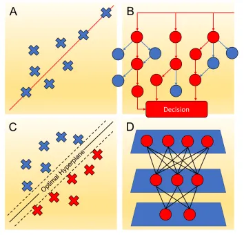
[image:15.595.114.468.282.622.2]These methods have seen widespread use in many fields.27 A disadvantage of MLR is the apparent ease of over-fitting. A useful rule of thumb is that the number of data points should be in excess of five times the number of explanatory variables (Fig. 1)26,27
Figure 1- Machine learning methods; (a) regression analysis aims to describe how the typical value of the dependent variable changes as the independent variables are changed. The regression function
(red line) characterises variation; (b) decision trees consisting of a binary separation at the nodes, leading to predictions or classifications at the leaf nodes (red circles); (c) an example of SVM separating data into distinct categories by an optimal hyperplane, which should have optimal margins either side for a clear distinction in data categorisation; (d) a typical neural network consists of layers of nodes. All nodes have connections with all other nodes in adjacent layers. The input units
(top) do not count as a layer of nodes, as they do not carry out any typical arithmetic operations. A typical arithmetic operation is the generation of a net signal and transformation by a transfer function into an output signal. The input units distribute input values to all of the neurons in the layer
Introduction
Random forest. Random Forest (RF), is a learning method based on decision or regression trees (depending on whether the predictive task requires classification or regression, respectively). These are stacked sets of binary separators following a tree like graph structure. RF uses a ‘forest’ of these decision trees, making use of “the wisdom of crowds”; hence, it is considered an ensemble learning method. For application to classification problems, the binary splitting is based upon the Gini index, which is a calculation of the maximal discrimination of the data points. For regression, splitting is generally based on a minimisation of the root mean squared error (RMSE). The initial node is known as the root node, with subsequent nodes being called branch nodes. The final nodes are referred to as leaf nodes and contain molecules with similar predictions of the property or activity (Fig. 1)28.
Support vector machines.Another commonly used machine learning method is that of Support Vector Machines (SVM). SVM supports both regression and classification tasks, and is capable of handling multiple continuous and categorical variables. Methods for handling classification tasks are based on typically non-linear kernel functions. These kernel functions allow the transformation of data points into a higher dimensional feature space (Fig. 1).
SVM training algorithms are built up of binary categorised data, whereby a particular data point belongs to one of two categories. Thus, the test set data is also categorised, producing a clear separation, which should be as wide as possible, in the feature space. Alternatively, in the case of regression, the surface behaves analogously to a regression line, providing a maximal explanation of the data within the bounds of an acceptable error margin whilst attempting to remain relatively flat to avoid overfitting.26,27
Networks. Artificial Neural Networks (ANNs) and deep learning architectures are another common form of machine learning method in chemistry. These are models conceptually based on the brain's neuron network (although a great simplification). ANNs contain an input layer which receives the molecular information, an output layer which provides the prediction to the user, and between these at least one hidden layer which is trained using data to link the neurons of the input layer and output layer in a suitable fashion for the problem at hand. The training generally involves weighting specific paths between the neurons.6,7,18 Deep learning algorithms attempt to abstract data on a high level through model architectures comprising multiple non-linear transformations. For example, in the case of ANNs the addition of hidden layers, which map some function of the input layer onto an output layer through a variety of unknown operations, can allow more information to be extrapolated from the input information.
1.2.3
The General Solubility Equation (GSE)
The GSE (as briefly mentioned in 1.1) is a QSPR model based on the melting point and the octanol– water partition coefficient log P of a chemical substance, used to predict the aqueous solubility of non-ionisable compounds,29 and acts as a useful guide for ionisable compounds using lipophilicity (log D) at the pH of the aqueous buffer employed. The equation states that;
789/ = 0.5 − 0.01 KN− 25℃ − 789X
Or in terms of log D;
789/?@(Y)= 0.5 − 0.01 KN− 25℃ − 789Z?@(Y)
[1.6]
The GSE is a simple QSPR model, with powerful predictive ability (coefficient of determination (r2) = 0.96 and root mean squared error (RMSE) = 0.53 log S units for a data set of 1026 organic molecules30), and the simplicity of the model means it has found wide application in the pharmaceutical industry. However, the reliance of the GSE on experimentally determined descriptors limits its applicability, and datasets sparsely populated at their limits can lead to overestimation of the model's predictive power.31
Ali et al.31 have revisited the GSE and have attempted to relieve the reliance of the GSE on the experimentally determined melting point by replacing it with the topological polar surface area (TPSA). They demonstrate the effects of inflated predictive power of the GSE by using a subset of an initial dataset, which reduced the overall predictive power of the GSE by approximately 6.4%. TPSA was included in a revised model to account for the fact that 88.5% of poorly performing compounds contained polarisable groups. The pure GSE model employed provided r2 = 0.818, and the TPSA replacement of melting point model provided r2 = 0.813, showing a comparable effectiveness. The number of compounds containing polarisable groups with log S predicted within ±1 log unit of experimentally determined values was also higher for the revised TPSA model (83.2% TPSA; 79.6% GSE). A final model combining melting point, log P and TPSA was also tested, and was found to have a better predictive power than both of the previously employed models (r2 = 0.869) with 90.8% of compounds containing polarisable groups predicted within ±1 log unit of experimentally determined values.
The work of Ali et al.31 highlights the importance of reliable descriptors in improving the overall performance of QSPR models, particularly when polar or polarisable functionality is included in test sets, and when experimentally determined values are required. As such, experimentally determined values may be best suited only for comparative analysis of predictive models to experimental data as a measure of performance in many cases.
1.3
Implicit solvation – the isotropic field as a
solvent representation
Continuum solvation models consider solvent as a continuous isotropic medium. An underlying assumption of implicit solvation models is that explicit solvent molecules may be removed from the model, provided that the continuous medium replacing them sufficiently represents equivalent properties.
A simplification of continuum models can be thought of in terms of a Hamiltonian as;
Ĥ\]\(^_) = Ĥ_(^_) + Ĥ_`(^_)
[1.7]
Introduction
in a continuum, rather than as definite atoms, as with explicit models. Ĥ_` is a sum of different interaction operators, which can be expressed in terms of solvent response functions, indicated by Qx(^′, ^′), where ^ indicates a position vector, and x represents a contributing interaction.
In a standard continuum model, generally represented by Polarisable Continuum Models (PCM), solute–solvent interaction energies can be represented by a number of Qx operators. The free
energy of M is therefore described by an expression of five terms;
G b = G42c+ Gd3+ G65(+ Ged?+ G0N
[1.8]
with the order of terms corresponding to the best performing order of the ‘charging processes’, which are integration processes coupling a distribution function with a potential function. The terms are the free energy of cavitation, electrostatic energy, dispersion energy, repulsion energy and thermal fluctuation, respectively.
1.3.1
Continuum models for electrostatic interactions
PCM models are advantageous in that they can represent a statistically averaged (continuum) solvent so that meaningful results can be acquired within a single calculation. PCM models have been particularly useful in modelling reactivity and spectroscopy of various solvents with different polarities.32
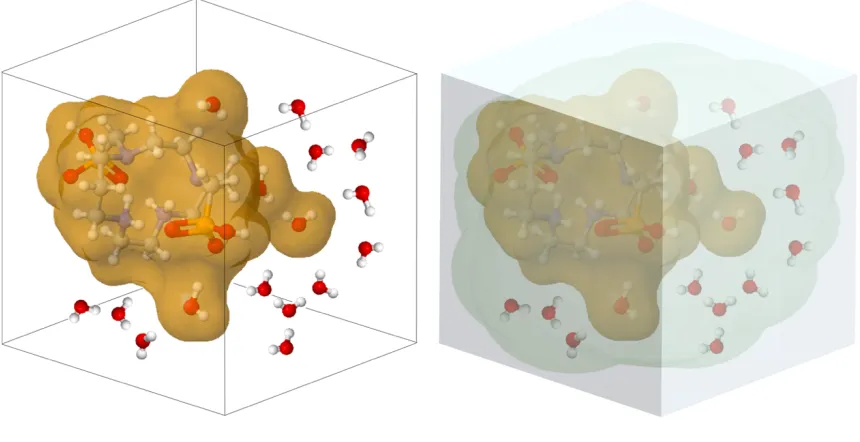
In a solvent–solute system where atom Q (solute) has a positive charge, solvent water molecules will preferentially orientate their negative dipoles towards the solute's positive charge (Fig. 2, left). For a single water molecule, there is only a slight preference in orientation, which is smaller than that of its average thermal fluctuations. Therefore, this effect is averaged over the long range of electrostatic interactions of water in the bulk (Fig. 2, right). For an isotropic solvent with random thermal motion, the average electric field is zero at any given point. However, introduction of a solute gives a net change in orientation, introducing an overall change in electric field, known as the ‘reaction field’.
Figure 2 - (left) Water molecules reorient themselves to preferentially point the negative end of their dipole towards the positive solute charge (+Q). (right) The system is modelled with a continuous
Accounting for the reaction field increases the solute's polarity proportionally to the solute polarisability, and the strength of the external electric field. This causes an increase in the dipole moment of Q, consequently polarising and increasing the change in orientation of the solvent to oppose the dipole moment of Q.3
There are energy costs associated with both the orientation and polarisation of the solvent, and the dipole moment of Q. As solvent molecules oppose the dipole moment of Q, they interact unfavourably with the reaction field. They also lose configurational freedom, with an associated free-energy cost. In a continuum model, the charge distribution of a solvent is represented as a continuous electric field, statistically averaged over all degrees of freedom at thermodynamic equilibrium. The electric field at any given point is the gradient of the electrostatic potential. The work required to create the charge distribution is determined from the interaction of solute charge density ρ with the electrostatic potential ϕ from;
G =1
2 f ^ g ^ !^
[1.9]
The polarisation component of G (GP) is the difference between charging the system in gas and solution phases; thus only the electrostatic potentials in both gas and solution phases are needed to calculate GP.
PCM methods are generally applied through two models; the Poisson–Boltzmann (PB) model, and the Generalised Born (GB) model. Both models are advantageous for different systems, and the accuracy of either model is mostly dependent upon the suitability of the cavity type used to surround the solute molecule within an ideal solvent system.
The Poisson–Boltzmann (PB) model. The Poisson equation combines the terms for electrostatic potential and the differential form of Gauss's law to define the electrostatic potential
g as a function of the dielectric constant ε and charge density ρ. When a surrounding dielectric medium responds linearly to an embedded charge, Poisson's equation states that;
∇ig ^ = −4kf(^)
l
[1.10]
Continuum solvation models represent the charge distribution on the basis of two separate areas: inside (solute) and outside (solvent) of a cavity (Fig. 3). For this case, the Poisson equation states;
∇l ^ ∙ ∇g ^ = −4kf(^)
[1.11]
The Poisson equation as expressed above is valid only for systems under non-ionic conditions. In a real solution, dissolving a solute produces mobile electrolytes. This effect is accounted for by an expansion of the Poisson equation, known as the Poisson–Boltzmann (PB) equation;
∇l ^ ∙ ∇g ^ − l ^ n ^ 8kp
iq
l%rK
%rK
p stuℎ pg ^
%rK = −4kf(^)
Introduction
where q gives the magnitude of electrolyte ionic charge, λ is a function equal to 0 in areas inaccessible to electrolyte ions and 1 for accessible areas, kB is the Boltzmann constant, and I indicates the ionic strength of the electrolyte system.
Figure 3 - An example of the solute cavity that may be calculated for a PCM calculation, represented by a solvent accessible surface area with a probe radius of 1.4Å (left) and an example of possible
points for field evaluation, represented by a dot-surface (right)
PB equations are best used to calculate the electrostatic potential of systems where the cavitation of solute is near-spherical or ellipsoidal (ideal cavitation), as the convergence of the predicted electrostatic component of the solvation free energy ΔGE is computationally expensive and often inaccurate. Thus, derivations applying approximations of the Poisson equation are often used in continuum models, the most common of which are Self-Consistent Reaction Field (SCRF) models,32 such as the Onsager model.33
A further limitation of PB based models is the definition of cavitation. A number of variational SCRF models have been proposed in order to optimise cavitation parameters, most commonly using tessellation (tiling) of the cavity surface to simplify and reduce iterations of the PB equation.32
The Generalised Born (GB) model. For systems in which ideal cavitation is not accurate, arbitrary cavitation can be applied. Arbitrary cavitation refers to the construction of a cavity around the solute similar to the shape represented by space-filling models generated from the overlap of atomic spheres at volumes representing van der Waals (vdW) radii. An alternative method to SCRF models involves an approximation of the Poisson equation that can be analytically solved, known as the Generalised Born (GB) approach.
A conducting sphere with charge q can be considered representative of a monatomic ion. If the surface of the sphere is assumed to be entirely smooth, the charge distribution around it will be uniform, and the charge density at any point is given by;
f s = p
4kwi
[1.13]
G = −1 2
p
4kwi −
p lw !s =
pi
2lw
[1.14]
The Born equation for the polarisation of a monatomic ion is calculated from the difference in the required work in the gas and solution phases applied to eqn. 1.14;
G?= −1/2 1 −
1 l
pi
w
[1.15]
The GB method extends the Born equation to polyatomic molecules to express polarisation energy as;
G?= −1/2 1 −
1
l pBpByzBBy
201N(
B,By
[1.16]
where k and kʹ run over all atoms, each with a partial charge q. The determination of suitable parameters for γ for polyatomic systems involves a radial integration of the charge q to determine the interaction of atom k with the surrounding medium. γ has units of reciprocal length, thus representing an inverse Coulomb integral. γ is given a suitable functional form in order to approximate the PB equation, and has a limiting behaviour, becoming closer to the exact reciprocal length r−1 at large interatomic distances.
1.3.2
Continuum models for non-electrostatic interactions
Similarly to the electrostatic components of solvation free energy, non-electrostatic contributions to the solvation free energy are not experimentally measurable. These contributions may have variable effects on the solubility of experimental systems. Various neutral model systems have been developed in accordance with this.
Specific component models. Pierotti34 developed a model formula, based on scaled particle theory, for the calculation of cavitation free energy through the observation of the solvation energy for noble gases. Scaled particle theory is a statistical-mechanical theory of fluids derived from exact radial distribution functions, to give an expression for the work required to place a spherical particle into a fluid of spherical particles. Noble gas atoms do not exhibit permanent electrical moments, thus their transfer into solution is considered to be the most analogous example of perfect cavitation.
The experimental data from Pierotti's work has been complemented by simulation data,35 including free energy of formation data of molecular-sized cavities in 12 common solvents obtained from free energy perturbation simulations. Pierotti's formula has since been expanded for molecular cavities by Colominas et al.36
Introduction
inducing a second instantaneous dipole, and so on, and an interaction occurs between these. The in-phase correlation of instantaneous and induced dipoles means the overall interaction energy does not average to zero over time.3 The average interaction energy falls off (largely) proportionally to r−6 (where r is the distance between interacting particles). The multipole expansion of the dispersion interaction is written;
M ^ ='| ^|−
'}
^}−
'~:
^~:…
[1.17]
where C6, C8 and C10 are dispersion coefficients dependent on the atomic species. This is normally evaluated as a sum over all pairs of atoms in different interacting molecules.
Atomic surface tensions. Another approach for the evaluation of the non-electrostatic components of solvation free energy assumes the non-electrostatic component to be atom or group specific, and proportional to atomic surface area. A recent review by Wang et al.37 (2009) considers four QSPR aqueous solubility models developed on the principle of weighted atom type counts and Solvent Accessible Surface Areas (SASA). They note that models considering SASA are often developed with small test-sets, and are therefore, in common with QSAR/QSPR models, poor performers for test molecules dissimilar to the original training set. The authors found that SASA descriptors did not enhance model performance any further than weighted atom type counts. This suggests the influences upon the non-electrostatic components of solvation free energy may be more complex than simple surface area considerations.
A further notable feature of continuum models based on surface tension is the neglect of any other contribution; that is, the development of these models assumes surface area as the sole determinant of solvation free energy, and that electrostatic components are implicit within the calculation parameters used.32
1.4
Explicit solvation models
Explicit solvation models are the primary choice of solubility models where solvent-specific effects are considered. The explicit treatment of water should, in principle, provide the most descriptive and realistic model for the investigation of solvation,38 however it intrinsically requires a large number of degrees of freedom and thus is associated with a phase space of high dimensionality. This requires statistical averaging over the entire phase space, particularly when extracting specific underlying physical behaviour, such as thermodynamic properties.
Statistical thermodynamics relates all observable thermodynamic properties to the partition function, Q. The partition function is summarised as;
Ä = ÅAÇ(É,?)BÑÖ !p!Ü
[1.18]
where Q is the classical formulation integrated over all phase space of all spatial q and momentum
1.4.1
Free energy calculations – Monte Carlo (MC) and Molecular
Dynamics (MD) simulations
Free energy considerations are distinctly different for intramolecular and intermolecular degrees of freedom. For intramolecular components, free energy contributions rely on vibrational and librational motions on an intramolecular energy surface.39 For well-defined energy-minima, the free energy is easily accessible from the partition function (eqn. 1.18) from vibrational frequencies treated with the harmonic approximation. The harmonic approximation estimates the nuclear potential of a molecular system in its equilibrium geometry at a potential energy surface minimum in terms of normal vibrational modes, each governed by a 1D harmonic potential. Anharmonic effects are accounted for with MC or MD simulations for the calculation of entropy on the intramolecular energy surface.39 Due to diffusion, the particles of a solution system do not exhibit motion definable by harmonic approximations. MC and MD simulations are restricted to only sampling the low-energy part of configuration space. Since internal energy and enthalpy are predominantly dependent on this low-energy region, they are well estimated. However, MC and MD methods do not involve the direct determination of Q, and exhibit an extremely slow convergence for densities of typical chemical systems, due to the exponential dependence of the Boltzmann factor on the energy, preferring the low-energy region. The high- and low-energy levels of molecular liquids are separated enough that typical MC and MD simulations will not sample the high-energy regions of configurational space necessary for an accurate calculation of the ensemble average of free energy39.
Free Energy Perturbation (FEP) methods. Free Energy Perturbation (FEP) methods were first introduced by Zwanzig40 in 1954, who related the thermodynamics of two different systems, in order to evaluate differences in intermolecular potentials. Zwanzig notes that at high temperatures, the forces of repulsion between molecules determine the equation of state of a gas, and that at lower temperatures the equation of state should be determinable by considering forces of attraction as perturbations on the forces of repulsion. The energy change from state A to state B is calculated by;
ΔG & ⟶ â = Gr− Gä
= −%rK 7u ÅTÜ −
ãr− ãä
%rK ä
[1.19]
where T is temperature, and the square brackets indicate an ensemble average over the simulation runs for A. A normal simulation run for A coincides with a new energy state of B on each optimisation run. The energy difference between A and B is either between the atoms in each state, or is an isomeric difference, for example A may be the cis-isomer of a structure, and B the trans-isomer, with A and B in different energy states due to different intra- and/or intermolecular interaction. For isomeric differences, the free energy map is calculated along a theoretical estimation of the reaction coordinates. The convergence of FEP calculations is only reliable for a small difference between A and B, thus traditional perturbation theory only holds true for systems which remain similar upon dissolution.
Introduction
into a series of intermediate transition state steps, allowing better convergence between the initial and final structures investigated.41 However, FEP calculations remain one of the most computationally expensive methods for calculating free energy differences.
An example of this is shown by Lüder et al.42 who have investigated the effectiveness of FEP methods for the calculation of free energy of solvation in pure melts for 46 drug molecules. Simulations were performed in two stages, scaling down the Coulomb and Lennard-Jones (LJ) interactions independently. Results were interpreted under the assumption that the free energy of the vapour to liquid process ΔGvl can be calculated from the sum of the free energy term for cavitation ΔGcav and the energy associated with LJ interactions and half of the Coulomb interaction term. ΔGcav is obtained from hard-body theories. Interaction energies and molar volumes for each of the 64 drug molecules were compared for systems comprising 260 molecules. Deviations between systems were found to be an average of 2.9% for intermolecular interaction energy, and 1.4% for molar volume, suggesting the dataset selected would provide reliable results. Predicted and simulated ΔGcav values were found to be systematically underestimated by approximately 15%. An overall average deviation of calculated ΔGvl values in comparison to experiment is −1.8 kJ mol−1, with reasonable errors expected in the range −1 to 1 kJ mol−1. This investigation suggests that overall, FEP methods require more work at the theory level, particularly due to systematic errors that occur in phase space relationships between reference and perturbed systems.
An alternative approach to calculating the free energy difference from one state to another is to treat the change from A to B as a transformation, rather than to calculate free energies of independent structures, and calculate an energetic difference, as in traditional FEP methods.3
A recent application of this method, derived from FEP, has been demonstrated by Liu et al.43 for the calculation of the solubility of gases in ionic liquids. The Bennett acceptance ratio (BAR) method utilises the method of transferring between states instead of treating each state as an individual structure. The Coulomb and LJ terms are calculated separately. It is found that simulated solubilities are found in good agreement with Henry's law constants. However, comparison to experimental data finds poorly soluble gases to have larger errors, with underestimated and overestimated gas solubilities found with similar calculation methods in complementary studies.
Enthalpy–entropy decomposition. A further offshoot of free energy calculations is the decomposition of the free energy term into enthalpic and entropic components.38 As both enthalpy and entropy are experimentally measurable, the difference between theory and experiment is ascertainable, and may be applied as benchmarks for force field optimisations,38 and give insight into the mechanism of solvation. Levy and Gallicchio have reviewed a variety of different approaches to the thermodynamic decomposition of free energies.38
values are statistically reliable and can be used for quantitative comparison to experimental data. The calculation of entropic and enthalpic contributions is also extremely computationally demanding, as every temperature point of a simulation requires recalculation of the overall free energy.3 Wyczalkowski et al. highlight that where calculation of free energies of solvation has advanced so that computational errors are on par with experimental ones, thermodynamic decomposition calculations suffer from statistical errors 10–100 times larger than free energy of solvation calculations.
A recent study by Ahmed and Sandler45 uses the decomposition of free energies of hydration and self-solvation of low polarity nitrotoluenes to consider an array of thermodynamic terms and physiochemical properties. These include: solid-phase vapour pressures, solubilities, Henry's law constants, hydration and self-solvation entropies, enthalpies, heat capacities and enthalpies of vaporisation or sublimation. Their study focuses on the temperature-dependence of various terms. Decomposition of hydration free energies into enthalpic and entropic contributions is performed by a method utilising polynomial fitting of temperature-dependent self-solvation free energies (with respect to temperature). The use of fitting increases the sensitivity of derived values of hydration free energies. Self-solvation enthalpy (ΔHself) values and entropy (TΔSself) values are calculated within approximately 2 kcal mol−1 of experimentally determined values.
1.4.2
Combined Quantum Mechanical/Molecular Mechanical
methodologies (QM/MM)
Explicit solvation models are often developed with respect to biological systems, due to the role of water in catalytic mechanisms, protein folding and protein–DNA recognition, to name but a few, which all require the specific detail of explicit water–substrate interactions to hold descriptive meaning. Of particular interest are combined QM/MM models, with QM describing electronic system changes (where precise system description is needed) and the rest of the system (where less precision is required) being described by a MM force field.3 Applications of QM/MM combined models are discussed in a recent review.46
The foundational concepts involve the partitioning of a desired system into two subsystems: the QM subsystem, containing a small number of atoms and described by QM, with the remainder of the system described by a suitable MM force field. The Hamiltonian of the whole system is simply written;
å = åçé+ åéé+ åçé/éé
[1.20]
where HQM is a QM Hamiltonian, HMM is an empirical force field and HQM/MM describes interactions at the QM/MM interface. The energy of the system is also described as the sum of QM, MM and QM/MM contributions. This model is often referred to as a two-layered approach (Fig. 4, left). A derivative of this model involves adding a third “layer” as a continuum solvent representation around the MM region, and is known as a three-layered approach (Fig. 4, right).
Introduction
provided by Friesner and Guallar46 for QM/MM methods applied to enzymatic catalysis, with descriptions, advantages and disadvantages of respective QM methods available in textbooks such as the one by Cramer.3
[image:26.595.91.521.232.453.2]A primary consideration when selecting a QM/MM method is the interactions at the QM/MM interface. Two aspects must be considered; (i) the presence of covalent bonds across the interface – a particular concern for large (e.g., biomolecular) molecules, and (ii) the influence of the MM solvent region on the QM region – electrostatic and van der Waals interaction terms must be included.
Figure 4 - (left) Two-layered approach to the QM/MM method. The solute molecule and a few water molecules are treated with QM (centre) and the rest of the solvent system is represented by MM up to a user-defined distance. (right) Three-layered approach – an additional layer surrounds the MM region and
uses a continuum approach to describe the long-range solvent in the bulk.
In order to treat covalent bonds at the interface, it is possible to introduce “link atoms”. Link atoms are QM hydrogen atoms that fill free valencies of QM atoms connected to MM atoms. A disadvantage of this method is the debate about inclusion of Coulombic interaction terms for the link atoms. Other methods developed in order to avoid the use of link atoms include the Local Self-Consistent Field (LSCF) method, which applies a mixture of hybrid and atomic orbitals to represent the QM system, and the “connection atom” method, where MM and QM interface atoms are described as QM methyl groups with a free sp3 valence.
the calculation with PCM, allowing less demanding calculations, and reduced sampling. However, three-layered approaches such as this often require much more user input and method manipulation, for example, considerations for MM/PCM interactions have to be considered in addition to QM/MM interactions, and so such methods are suited only to experts.
1.4.3
Explicit representations of water atoms
When solvent is represented explicitly, solvent molecules usually greatly outnumber solute molecules. Thus, in order for a model to be efficient, it is advantageous to use the simplest possible solvent representation.48 Water is often considered the most useful solvent system, and thus is the solvent most widely used in explicit solvent models. The macroscopic properties are well established, yet the microscopic forces that determine water structure are not fully understood.
The treatment of water can be rigid or flexible. Rigid models often include a fictitious H–H bond to constrain bond angles in the water monomer.3 Three of the most common rigid models for water are the TIP3P (transferable intermolecular potential 3P), SPC (simple point charge) and SPC/E (simple point charge extended) models, and their modified counterparts. These three models are effectively rigid pair potentials comprising LJ and Coulombic terms. However, the terms used differ in each model, and give rise to different calculated bulk properties for water.48 Values for various properties of water obtained with different rigid models of water are shown below, in Table 1.
Table 1 - Model vs. experimental (exp.) values for bulk properties of water under standard conditions (298 K; 1 bar), including dipole μ, density ρ, static dielectric constant ε0 and heat capacity Cp
Property TIP3P49,50 TIP4PEw51 SPC/E50,52 Exp.50
μ (D) 2.348 2.32 2.352 2.5–3.0
ρ (g cm−3) 0.980 0.995 0.994 0.997
ε0 94 63.90 68 78.4
CP (cal K−1 mol−1) 18.74 19.2 20.7 18
Introduction
Spoel et al.53 (1998) investigated the effectiveness of TIP3P, TIP4P, SPC, and SPC/E models in describing the density and energy, dynamic, dielectric and structural properties of water. All simulations and analyses were identical for each model investigated, allowing the evaluation of simulation methodology independent of the model. It was found that system size, cut-off length and reaction fields had comparable effects on the overall calculated structural properties of water.
System size effects are considered through the comparison of systems comprising a small (216) and a large (820) number of molecules. The average thermodynamic properties (ρ, Epot, T, P) are the same regardless of system size. Fluctuations in thermodynamic properties are known to be proportional to the square root of the system size, which is confirmed within the study. However, differences between large and small systems are observed, particularly for the dielectric constant, which is higher for all systems with a large number of molecules. The diffusion constant for large systems is also higher, attributed to periodic boundary conditions (PBC).
Cut-off effects are considered by the use of two different cut-off lengths (9 Å and 12 Å) for the large systems. It is found that density increases with an increased cut-off length, and energy decreases. There is no effect on dielectric behaviour.
In all simulations density is reduced, and the energy is decreased by approximately 1 kJ mol−1 on application of a reaction field. The self-diffusion constant D, and rotational correlation times were found to increase, indicating that the reaction field affects both the translational and rotational mobility of molecules.
Quantum chemical MD simulations of water are often developed with Density Functional Theory (DFT) methods, using either plane wave or atom-centred basis sets, to determine the electronic structure and forces. These methods offer reasonable estimates of the structural and dynamic properties of water when compared to experimental measurements. However, problems exist in the description of electronic gradient corrections, and equilibrium pressure. The interatomic forces of early quantum simulations, including DFT based methods, were originally parameterised with classical mechanics, leading to an unsatisfactory agreement between quantum and experimental results. DFT models also tend to calculate liquid structure with too much order, and underestimate equilibrium density. This is often attributed to the inability of local functionals to describe dispersion effects.
mol−1. Scaling the dispersion term results in an increased equilibrium density for increased dispersion. This induces a weakening effect on the H-bonding network of water, bringing the overall structure closer to agreement with benchmark data. However, the calculated ΔHvap increases to 46 ± 2 kJ mol−1, which is 4% higher than the experimental value. It is also found that the H-bond network is sensitive to changing polarisation at fixed dispersion, affirming the independent importance of both polarisation and dispersion effects on an overall explicit model.
1.5
Hybrid models
Within an aqueous solution phase, single snapshot images of structure are of limited use. Water is one of the few single component liquids for which there are highly competitive interactions at short range (hydrogen bonding), capable of damping the effects of repulsion. For this reason, ensemble averaging is required to identify the most probable geometric configurations which most heavily contribute to the system's interactions. This idea has already been introduced within explicit models of solvation, using ensembles taking snapshots at specific time periods. However, the cost of calculating the many configurations accessible in a solution is enormous. A number of methods, based on statistical mechanics, enable a more efficient calculation process.
1.5.1
Correlation functions
From a chemical point of view, a solution is a highly mobile system in which the dynamics are a vital contribution to the system's properties and behaviour. Therefore, mathematically we wish to capture this. Attempting to quantify dynamics with static properties is not sufficient; we must therefore provide averages or probabilities of interactions occurring at given distances. For this reason, a natural choice is to represent the solvent using Pair Correlation Functions (PCF), or equivalently Radial Distribution Functions (RDF). These functions allow us to determine a probabilistic structure of the solvent.
PCF can be interpreted as showing the probability against distance of there being an atom of interest at that distance from the atom under study. For example, the first large blue peak in Fig. 5 would correspond to either a water H at a distance from an O atom under study or vice versa. These functions are experimentally determinable from scattering experiments. We would expect that the PCF/RDF would go to a constant value of 1 at large values of r (i.e. it would become isotropic, like a continuum model, as there are no solute interactions to perturb the system). However, at small values of r we would not expect this. At very small values (less than the van der Waals radii of the solute atoms) we expect zero as only one particle can occupy the space at a time. Just outside this distance we see sharp non-uniform behaviour as solvent in the space interacts favourably with the solute holding a more rigid form. This leads to troughs in the PCF/RDF just behind the peaks, thus deviating from the value of 1 for a uniform solvent (Fig. 5).
Introduction
fundamental 6D integral equation, the Molecular Ornstein–Zernike equation (MOZ). This equation utilises PCF/RDF between the various constituents of the liquid, g(r1, r2, Θ1, Θ2). This simplifies for homogeneous solution to relative positions and orientation of the constituents, g(r1 − r2, Θ1 − Θ2). This can most conveniently be written with reference to the total correlation function h(r,Θ).55
ℎtè ^1− ^2, Θ1− Θ2 = 9tè ^1− ^2, Θ1− Θ2 − 1
[1.21]
Figure 5 - A schematic representation of PCF for liquid water; water oxygen – water hydrogen (blue), water oxygen – water oxygen (orange) and water hydrogen – water hydrogen (grey).
We can simplify this equation by assuming spherical symmetry of molecules, hence removing consideration of orientational degrees of freedom by treating each water molecule as a hard sphere. This simplification leads to a 1 dimensional treatment of the integral, known as 1D-RISM (it is more accurate to treat the integral in 3D). We can now further separate the contributions to the total correlation function into direct and indirect components. To do this we must introduce the direct correlation function c(r). We can now re-write the equation 1.21 assuming spherical symmetry as follows:
ℎ ^~,i = ë ^~,i + !^íë ^~,í f ^í ℎ ^i,í
[1.22]
Two effects contribute to the total correlation function (eqn. 1.22); (i) the direct correlation between r1 and r2, and (ii) an indirect correlation via a third body, r3. The indirect correlation via
r3 is weighted by the density at r3, and thus allows the consideration of all possible positions of the third body (Fig. 6).56
To solve this equation, h(r) and c(r) need to be found. As we have only a single equation and two unknown functions, h(r) and c(r), another equation is required; a closure relation must be introduced. There are several such equations available from statistical mechanics. The exact closure relation is as follows:
9 ^ = ÅAìî e ïñ e A4 e ïr(e)⟹ ÅAìî e ïÖ e ïr(e)
[1.23]
where ò is equal to 1/kBT and U(r) is the interaction potential which is often of the following form:
ô ^ = 4l ö2E ^
~i
− ö2E ^
|
+p2pE ^
[1.24]
where lis the depth of the potential well, and öis the finite distance for which the inter-particle potential is zero. T(r) is known as the indirect correlation function as it is the difference between the total and direct correlation functions, and quantifies the indirect contribution. B(r) is the bridge function, which comes from graph theory – its exact form is not known. Several approximate closure relations exist; some will be discussed here, although others are available. Originally the HyperNetted-Chain (HNC) approximate closure was used:
ℎ ^ = Å Aìî e ïÖ e − 1
[1.25]
This closure works in principle for charged systems but neglects the bridge function term completely, assuming it to be zero. This can lead to poor convergence due to uncontrolled growth in the argument of the exponent. An alternative is the Partially Linearised Hyper-Netted Chain (PLHNC). This closure linearises the HNC once a cut off value (C) is exceeded;17
Λ = −òô ^ + K ^
ℎ ^ = −òô ^ + K ^ + ÅÅ(Aìî e ïÖ e )ú− 1− ' − 1 ùℎÅu Λ ≤ 'ùℎÅu Λ > '
[1.26]
This improves the convergence of the equations and is now regularly used in many applications for a variety of systems.
Due to the spherical symmetry approximation, the MOZ can only be applied to simple solutions. Additionally, due to the high dimensionality of the full equation, before the spherical symmetry approximation was invoked, it was practically incomputable. For this reason, a number of approximations have been developed which are collectively referred to as Reference Interaction Site Models (RISM).57,58
Theory & Methods
This thesis investigates the improvement of solubility prediction. The methods involved within the projects discussed herein are primarily focused on data-mining and informatics, utilising empirical data from a number of sources. The primary data for all of the methods used comes from the Cambridge Crystallographic Data Centre’s (CCDC) Cambridge Structural Database (CSD). Other data comes from a variety of sources, which will be detailed with respect to each method in their own chapters. This chapter discusses the fundamental theories and methods explored and applied in this thesis.
2.1
Crystallography
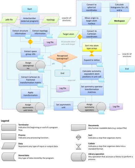
The unit cell of a crystal structure contains a group of atoms with a fixed geometry relative to one another. The intrinsic highly ordered symmetry of crystal structures gives rise to geometrical and symmetrical relationships known as symmetry elements and operators. These operators are determined from the original diffraction pattern of a crystalline material during crystal structure solution and refinement. The symmetry properties of crystal structures are described by spacegroup notation. The spacegroup of a crystal structure is specific to the translation of atom positions of the asymmetric unit, within the unit cell, to positions with a symmetrical equivalence
(i.e the symmetry of every crystal structure with the same spacegroup can be determined through the same translation matrix operations to fill the unit cell with symmetry equivalent atom points). These translations are specified in three dimensions, in terms of the unit cell parameters. The unit cell parameters define the length of the three unit cell edges in the x, y, and z direction, and are notated a, b and c. The angles between the unit cell axis are notated α, β and γ.
The translational symmetry operations of the asymmetric unit to give atom positions of the unit-cell are often computed through black box operations within a computer program, however, this can be done manually by application of the symmetry operations as described within the “International Tables of Crystallography: Volume A.”61
Within the “Tables for Crystallography”, space groups are denoted by International short Hermann-Mauguin symbols, which represent space groups in two parts. The first part is a letter describing the centring of the space group (e.g. P for primitive or F for face-centred), and the second part is a set of characters representing the symmetry elements of the space group. The space groups are also represented in terms of space-group diagrams, which show the relative locations and orientations of symmetry elements, and the arrangement of symmetry equivalent points.
2.1.1
Transformations of the coordinate system
Symmetry operations are transformations by which the coordinate system and the origin are considered to be at rest, whilst the ‘object’ or molecule(s) is mapped onto itself. The coordinate system can be considered as the basis vectors a, b and c, and the origin 0. A symmetry operation
W transforms every point X with the coordinates x, y, z to the point † with coordinates T, R, °. In matrix notation, this transformation is equivalent to62;
T R °
=
ù~~ ù~i ù~í
ùi~ ùii ùií ùí~ ùíi ùíí
T R ° + ù~ ùi ùí =
ù~~T + ù~iR + ù~í° +
ùi~T + ùiiR + ùií° +
ùí~T + ùíiR + ùíí° +
ù~
ùi
ùí
[2.1]
The 3x3 matrix (W) represents the rotation part of the symmetry operator, and the column matrix
(w) the translational part of the symmetry operation. W, w characterises the symmetry operation uniquely. This can be simplified by the use of an augmented 4x4 matrix;63
" = " ù
0 1 =
ù~~ ùi~ ùí~ ù~i ùii ùíi 0 0 ù~í ùií ùíí 0 ù~ ùi ùí 1 [2.2]
This augmented matrix allows the calculation of the points T, R, ° by;
T R ° 1 = ù~~ ùi~ ùí~ ù~i ùii ùíi 0 0 ù~í ùií ùíí 0 ù~ ùi ùí 1 T R ° 1 =
ù~~T + ù~iR + ù~í° + ùi~T + ùiiR + ùií° +
ùí~T + ùíiR + ùííz +
ù~ ùi ùí 1 = £ = §£ [2.3]