The Development of Self Balancing Controller for One Wheeled Vehicles

Engineering, 2010, 2, 212-219

doi:10.4236/eng.2010.24031 Published Online April 2010 (http://www.SciRP.org/journal/eng)

The Development of Self-Balancing Controller for

One-Wheeled Vehicles

Chung-Neng Huang

Graduate Institute of Mechatronic System Engineering, National University of Tainan, Taiwan, China E-mail: [email protected]

Received November 30, 2009; revised February 16, 2010; accepted February 19, 2010

Abstract

The purpose of this study is to develop a self-balancing controller (SBC) for one-wheeled vehicles (OWVs). The composition of the OWV system includes: a DSP motion card, a wheel motor, and its driver. In addition, a tilt and a gyro, for sensing the angle and angular velocity of the body slope, are used to realize self-balancing controls. OWV, a kind of unicycle robot, can be dealt with as a mobile-inverted-pendulum system for its instability. However, for its possible applications in mobile carriers or robots, it is worth being further developed. In this study, first, the OWV system model will be derived. Next, through the simulations based on the mathematical model, the analysis of system stability and controllability can be evaluated. Last, a concise and realizable method, through system pole-placement and linear quadratic regulator (LQR), will be proposed to design the SBC. The effectiveness, reliability, and feasibility of the proposal will be con- firmed through simulation studies and experimenting on a physical OWV.

Keywords: Self-balancing Controller, One-wheeled Vehicle, Mobile-inverted-pendulum, Pole-placement, Linear Quadratic Regulator (LQR)

1. Introduction

In recent years, because of the surging consciousness of global pollution and energy-shortage crises, automobiles and motorcycles are no longer the best for transportation. In order to fit the daily required and improve above problems, exploring new energy or developing lighter and innovative mobile carriers are beginning to be known as new trends. The earliest two-wheeled balanc-ing robot was published in 1987 by Prof. Yamafuji [1]. From then on, the concerning researches with this topic have been increasing [2-6] and have even been a com- mercialized product. For example, the Human Trans- porter, was developed by Segway Co., U.S.A., which is a very famous two-wheeled balancing vehicle [7,8]. In addition, NASA’s Robonaut, Segway platform puts ro-bots in motion, is now aim in the military projects [9].

However, the balancing mechanism of a two-wheeled system is rather complicated. Whereas, for the problems, the two-wheeled synchronization and body balancing should be considered simultaneously, making a lot of sensors a requirement. It does not only complicate the system, but also increases the cost. For the reasons above,

how to simplify the two-wheeled system has become one of the studying motives of OWV. By this motive, not only can it maintain the advantages of a two-wheeled system, but it can also simplify the system mechanism further, decreasing the cost.

Nowadays, although a lot of references engaging in the studies of two-wheeled balancing carriers can be found [2-6], the ones for OWV studies are still insuffi-cient [10,11]. Trevor Blackwell [12], an American engi-neer, has proposed an OWV design on his personal web-site, and the concept OWV, EMBRIO, is published by BRP [13], a motorcycle manufacturer in Canada. Besides, [10] is the newest one based on fuzzy controls for bal-ancing.

C. N. HUANG 213 complete knowledge [4,14]. However, it has not been

viewed as rigorous due to lack of formal synthesis tech-nologies, which guarantee the basic requirements for control systems such as global stability [15]. That is, it is not only difficult to precisely know the mutual influ-ence between each system state but also might be diffi-cult and expensive to design the controller for its com-plexity highly depending on the number of fuzzy rules [16].

Consequently, finishing system modeling and analy-sis for proposed SBC is set as the first step of this study. Next, by linearizing the system model, pole-placement and state-feedback controls can be found and designed. Finally, through human-computer interaction, a DSP card featured with motion control is adopted to handle the real-time computation of digital signals.

However, from above studies found that only using the pole-placement and state-feedback controls, the feedback gains can not be adjusted easily. It is difficult to lead the system in a better stability. Here, LQR is used to improve the above problems. For comparison, both the numerical and experiment studies on SBC, basing on pole-placement and LQR controls, respectively, are made. The studies have proved that the proposed SBC is able to perform higher controllability and stability.

2. Modeling for OWV

The concept of the OWV prototype is simply constructed by a wheel motor and two sensors as a tilt and gyro. Here, the wheel motor is adopted as the driving wheel of the OWV that uses the feedback signals from sensors to balance the system body. Figure 1 shows the outward appearance of OWV prototype where the box on the upper side of wheel motor can be treated as the balancing weight of inverted-pendulum, and in which the motor driver, sensors are set. Figure 2 shows the free body diagram of OWV in Figure 1.

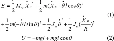
According to the free body diagram in Figure 2, the kinetic energy E and potential energy U can be expressed as follows, respectively.

2 2 2 2 2 ) ( 2 1 2 1 ) sin ( 2 1 ) cos ( 2 1 2 1 R X J J l m l X m X M E M w m w w w                   (1)  cos mgl mgl

U   (2) Basing on Lagrange’s equation as well as the coeffi-cient transformation for deriving mathematic model of OWV, the Lagrange equation can be written as:

R T X L X L dt d w w w               

Figure 1.OWV prototype.

Figure 2.Free body diagram of OWV.

0                _  L L dt d (3) where LEU

From (3), the accelerations of body movement and in-cluded angle between vertical axis and body can be found as follows.

m w w m w w J ml l m R J m M J ml g l m ml R T X            2 2 2 2 2 2 2 2 2 cos cos sin sin      (4) 2 2 2 2 2 2 2 cos sin ) sin ( cos R J m M l m J ml mgl R J m M ml R T ml w w m w w w                 

 (5)

Since (4) and (5) are nonlinear equations, for simpli-fying and modeling, let them be represented on the

bal-anced point   0 and given ₂ R J m M M w w

C. N. HUANG 214

x

J

S

1 Xw

w

X

w

X

S 1 S 1  J 1  K w

T



Figure 3. OWV control (linear).

the equations can be rewritten as

R l m J ml R M T J ml l m J ml M g l m X m e m m m e w 2 2 2 2 2 2 2 2 2 ) ( ) ( ) (            (6) R l m J ml R M mlT l m J ml M mglM m e m m e e 2 2 2 2 2

2 _{) ( )}

(         

 (7)

By using (6) and (7), the block diagram for OWV control can be illustrated as shown in Figure 3. Where,

] ) (

[ 2 22

2 l m J ml M R J ml J m e m

x _{ }

  ， 2 2 2 2 2 )

(ml J ml

M g l m K m e

x _{ }

  R l m J ml R M ml J m e 2 2 2 ₎ (    

 ，K MegR

From Figure 3, it can be found that OWV is a sin-gle input and multiple output system (SIMO). Besides, OWV is similar to the inverted-pendulum vehicle, belonging to the non-minimum phase system [3,17].

3. Analysis and Design for State Variables

3.1. Performance of System Instability

Since a system can be represented in state space by fol-lowing equations:

Bu AX

X   (8)

y CX Du (9)

for and initial conditions with respect to the equilibrium point, , where

0

t t



) 0 , 0 , 0 , 0 ( ) (t0 

X X: state vector



X: derivative of the state vector with respect to time

y: output vector

u: input or control vector

A: system matrix B: input matrix C: output matrix D: feed forward matrix

(8) is called the state equation, and the vector X, the state vector, contains the state variables. It can be solved for the state variables. Besides, (9) is called the output equation. This equation is used to calculate any other system variables.

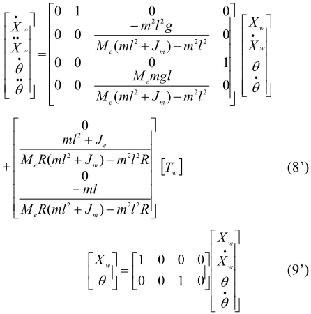
For the linear, time-invariant, second-order system as OWV, its system dynamics can be transformed and ex-pressed by state equations; the state space of OWV can be taken on the following form by (6) and (7).

                      w w X X =                      0 ) ( 0 0 1 0 0 0 0 ) ( 0 0 0 0 1 0 2 2 2 2 2 2 2 2 l m J ml M mgl M l m J ml M g l m m e e m e                   w w X X +                       R l m J ml R M ml R l m J ml R M J ml m e m e e 2 2 2 2 2 2 2 ) ( 0 ) ( 0

 

                                w w w X X X 0 1 0 0 0 0 0 1 (9’)

In order to confirm the effectiveness of the derived model, through the simulation by mechanical design software Solidworks, or CATIA, system analysis and estimation of system coefficients are done.

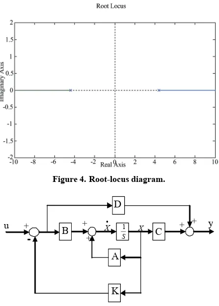
Table 1 and Figure 4 show the estimated system co-efficients of OWV by Solidworks’ analysis.

Based on above, system coefficients and system sta-bility, the analysis finds that for OWV it is not a stable system. Initially, it would fall down by an outside dis-turbance. This phenomenon can be confirmed by the root locus as shown in Figure 4. Where, for one of the poles locating in the right of s-plane, it can be judged that it is an unstable system. Besides, this result also can be con-firmed by finding out the eigenvalues of system matrix in (8’) ass0,0,4.4116,4.4116.

Table1.System coefficients of OWV.

m 4.31 kg

Jm 0.1984 kg-m2

l 0.1 m

R 0.07 m

Mw 5.1819 kg

C. N. HUANG 215 3.2. Analysis for the Controllability of OWV

Accepting to discuss the system stability in state-space analysis, the controllability of system is also an impor-tant index. That is, before designing state-feedback con-trollers, the analysis for controllability should be done in advance to make sure the system is able to achieve the desired responses through state-feedback control and observing.

Pole-placement is a viable design technique only for systems that are controllable. In order to be able to de-termine controllability or, alternatively, to design state feedback for a plant under any representation or choice of state variables, a matrix can be derived that must have a particular property if all state variables are to be con-trolled by the plant input, u. For an nth-order plant whose state equation is (8), which is completely controllable if the matrix

Figure 4.Root-locus diagram.

S 1



X ＋

＋

＋

＋

B X _C

A

y D

K

-

u ＋

2 n

c

Q _B AB A B A 1B_

    (10)

is of rank n, where is called the controllability matrix. Now, by substituting the coefficients of Table 1 to the system and inputting matrices in (8’) and using (10), then

c

Q

 

rank can be found. That is, OWV is completely controllable on the balancing point. Its closed-loop sys-tem’s poles can be placed at desired locations on the s-plane through using the state feedback u(t)Kx(t).

Figure 5.State-feedback block diagram.

3.3 State-Feedback Control In order to improve the system instability, the state

feedback as well as the pole-placement design is adopted to make the system stable and balanced. By which, the block diagram of the system state feedback is shown as Figure 5. Where, the feedback is given asuKx(t).

In Figure 5, for the system feedback uKx(t) , the closed-loop system matrix can be expressed as

] [k1 k2 k3 k4

    

 

    

 

 

 



 



 

4 3

2 1

4 3

2 1

2696 . 2 2696 . 2 4625 . 19 2696 . 2 2696 . 2

1 0

0 0

2717 . 1 2717 . 1 6987 . 0 2717 . 1 2717 . 1

0 0

1 0

k k

k k

k k

k k

BK

A ₍₁₁₎

Thus, the transfer function of the closed-loop system det





1 2 3 4

1 2 3 4

1 0 0

1.2717 1.2717 0.6987 1.2717 1.2717

0

0 0 1

2.2696 2.2696 19.4625 2.2696 2.2696

s

k s k k k

s

k k k s k

 

_{    } 

 _{ }

 

 

 

 

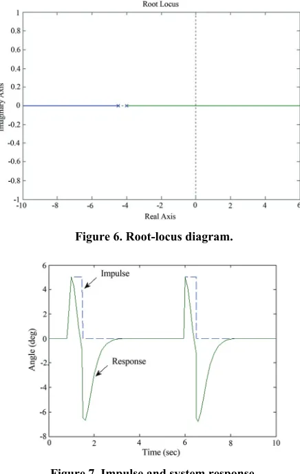
Here, assume an example for placing the system’s poles at s= 0, 0, -4.5, -4, since the system transfer function should satisfy the condition _{s s}2









, the feedback gains of system state can be found as . In order



16 0 0 ]

[ 1 2 3 4  

 k k k k K

C. N. HUANG 216

Figure 6. Root-locus diagram.

Figure 7. Impulse and system response.

motion, still can return to the desired balancing state as shown in Figure 7.

3.4 LQR Control

In above section, it shows that pole-placement and state-feedback controls used for SBC are available and realizable. However, if the unstable pole could only be placed in the left of s-plane by using assignments (ex-perienced studies), then adjusting the feedback gains to a better stability for OWV would be difficult.

In order to improve above problem, LQR, the con-tinuous time infinite horizon linear quadratic regular with control constraints, is adopted to design SBC. Determi-nistic LQR theory was first introduced by Kalman, and has been playing a central role in modern control theory as well as various engineering practices; the reader can be referred to the well-known book [18], as the following problem:

Minimize quadratic performance index



J T T

 

 

0 () () () ()



Here, the state vector is locally abso-lutely continuous, and the minimization is carried out over all locally integrable controls . Throughout the note, the standing assumptions are

n

IR X:[0,)

u_{:[0,)IR}k

1)Q and R, the weighting matrices of X(t) and

) (t

u , are symmetric and with positive semi-definite and positive definite, respectively.

2)The pair (A, B) is controllable. The pair (A, C) is observable.

3)The set U is closed, convex, and 0intU.

For the unconstrained problem (8), (9), and (12), the optimal solution of the problem is the following state-feedback control.

) ( ) ( )

(t K t X t

u  (13)

where, , and P, the unique symmetric and positive definite matrix, is the solution of the Riccati differential equation as

) ( )

(_{t R}1_{B P t}

K _  T

Q t P B BR t P t P A A t P t

P_{() () } T _{() ()} 1 T _{() (14)}

Since there is only stable state considered for OWV system, that isP(t)0, (14) can be rewritten as

Q P B PBR P A

PA_ T _ 1 T _{ (15)}

By substituting (15) into (13) with system coeffi-cients, , the optimal feedback gains, can be found as

)

(

t

K

1 2 3 4

K_k k k k _





 

] 1 [

, by giving matrices R , and Qdiag([10 1 1 1]). The R and Q are provided to have constraint of control action satisfied.

Figure 8 shows the comparison of stability responses by using pole-placement and LQR, respectively. Where, SBC, basing on LQR control, let OWV have a better system stability is confirmed.

4. Physical Demonstration of

For further confirming above numerical studies and the feasibility of OWV, the testing setup is accomplished and pictured in Figure 9.

A motor driver and sensors (SSY0090 tilt and CRS03- 02 gyro) are set in the box and a 24-V 250-W wheel mo-tor (SA176-6) [19] is used as the driving wheel. All the algorithms for pole-placement, feedback-gain calculation, and LQR etc. are developed with C language and im-plemented in an ITRI PMC32-6000 DSP board with a clock frequency of 40MHz (Figure 10).

C. N. HUANG 217

Figure 8. Comparison of stability responses.

Transforms Low pass filter

body State feedback

A/D CPU

D/A A/D

Driver

DSP

Tilt Gyro

Figure 9. OWV setup.

Figure 11. Control block diagram of OWV.

terrupting algorithm is executed by every 1 ms.

Figure 12 shows the voltage outputs of motor control, angular signals of OWV’s body from gyro and tilt while SBC bases on pole-placement and LQR controls, respec-tively. Here, by examining angular velocity (Figure 12(b)), since it, the derivatives of body tilt angle can be taken as the estimation of next-state body falls, the

Figure 10. DSP board.

C. N. HUANG 218

(a) voltage outputs

(b) angular velocity

(c) tilt angle

Figure 12. Control signals.

voltage signal (Figure 12(a)) is approximately inverse to angular velocity for falling-preventive control. Be-sides, in Figure 12(c), even through some tiny oscilla-tions within 2 degree occur when the body of OWV is starting to swing up by the wheel-motor driving a horizontal force to move OWV back and forth, after 3.75 seconds it can return to the desired balancing state. Consequently, it proves that SBC is able to be realized by both above controls. Moreover, through the comparisons of the signals in Figure 12, finds that the magnitude of the state signals by LQR control is smaller than those by pole-placement control. It is not only shows LQR with better system stability per-formance but also corresponding to the objective of LQR control in (12).



5. Conclusions

This study has proposed a SBC, based on concise con-struction and control theories for OWV. Only based on state-space modeling and real-time sensing, the SBC is attractive for its conciseness and feasibility. Studied sults show that the real-time SBC is not only can be re-alized but also can let OWV with optimal stability by LQR control.

By further developing OWV technologies, such as SBC etc., the benefits not only can serve the handling problems, existing in present electrical mobile-robots, welfare carriers, or two-wheel entertainment vehicles as large steering radius (angle), differential gear, or syn-chronization control etc., but also with advantages on cost, setup, light quantity, and saving energy, etc.

6

. References

[1] Z. Sheng and K. Yamafuji, “Postural Stability of a Hu-man Riding a Unicycle and Its Emulation by a Robot,”

IEEE Transactions onRobotics and Automation, Vol. 13, No. 5, 1997, pp. 709-720.

[2] Y.-S. Ha and S. Yuta, “Trajectory Tracking Control for Navigation of the Inverse Pendulum Type Self-contained Mobile Robot,” Robotics and Autonomous Systems, Vol. 17, No. 1-2, 1996, pp. 65-80.

[3] F. Grasser, A. D’Arrigo, S. Colombi and A. C. Ruffer, “JOE: A Mobile, Inverted Pendulum,” IEEE Transac-tions on Industrial Electronics, Vol. 49, No. 1, 2002, pp. 107-114.

[4] S. Jung and S. S. Kim, “Control Experiment of a Wheel- Driven Mobile Inverted Pendulum Using Neural Net-work,” IEEE Transactions on Control Systems Technol-ogy,Vol. 16, No. 2, 2008, pp. 297-303.

[5] K. Pathak, J. Franch and S. K. Agrawal, “Velocity and Position Control of a Wheeled Inverted Pendulum by Par-tial Feedback Linearization”, IEEE Transactions on Ro-botics,Vol. 21, No. 3, 2005, pp. 505-513.

[6] Y. Kim, “Dynamic Analysis of a Nonholonomic Two- Wheeled Inverted Pendulum Robot,” Journal of Intelligent and Robotic Systems, Vol. 44, No. 1, 2005, pp. 25- 46. [7] H. Tirmant, M. Baloh, L. Vermeiren, T. M. Guerra and M.

Parent, “B2, an Alternative Two Wheeled Vehicle for an Automated Urban Transportation System,” Proceedings of IEEE Intelligent Vehicles Symposium, Vol. 2, 2002, pp. 594-603.

[8] D. Voth, “Segway to the Future [autonomous mobile ro-bot],” IEEEIntelligent Systems, Vol. 20, 2005, pp. 5-8. [9] R. O. Ambrose, R. T. Savely, S. M. Goza, P. Strawser, M.

A. Diftler, I. Spain and N. Radford, “Mobile Manipulation using NASA’s Robonaut,” Proceedings of IEEE Interna-tional Conference on Robotics and Automation, New Or-leans, 2004, pp. 2104-2109.

C. N. HUANG 219 [16] C. W. Tao and J.-S. Taur, “Flexible Complexity Reduced

PID-like Fuzzy Controllers,” IEEE Transactions on Sys-tems, Man, and Cybernetics, Part B, Vol. 30, No. 4, 2000, pp. 510-516.

[11] K. Hofer, “Observer-Based Drive-Control for Self- Balanced Vehicles,” Proceedings of IEEE /IECON 32nd Annual Conference on Industrial Electronics, 2006, pp. 3951-3956.

[12] The Electric Unicycle, Available: http://tlb.org/eunicycle.html [17] M. I. El-Hawwary, A. L. Elshafei, H. M. Emara and H. A. Abdel Fattah, “Adaptive Fuzzy Control of the Inverted Pendulum Problem,” IEEE Transactions on Control Sys-tems Technology, Vol. 14, No. 6, 2006, pp. 1135-1144. [13] EMBRIO, Available: http://www.brp.com/en-CA/

[14] C. W. Tao, J. S. Taur, T. W. Hsieh, C. L. Tsai, “Design of a Fuzzy Controller With Fuzzy Swing-Up and Parallel Distributed Pole Assignment Schemes for an Inverted Pendulum and Cart System,” IEEE Transactions on Con-trol Systems Technology,Vol. 16, 2008, pp. 1277-1288.

[18] B. Anderson and J. Moore, “Optimal Control-Linear Quadratic Methods,” Prentice-Hall, Upper Saddle River, 1990.

[19] Y.-P. Yang, D. S. Chuang, “Optimal Design and Control of a Wheel Motor for Electric Passenger Cars,” IEEE Transactions on Magnetics, Vol. 43, No. 1, 2007, pp. 51-61.

[15] R. J. Wai, M. A. Kuo, J. D. Lee, “Cascade Direct Adap-tive Fuzzy Control Design for a Nonlinear Two-Axis In-verted-Pendulum Servomechanism,” IEEE Transactions on Systems, Man, and Cybernetics, Part B,Vol. 38, 2008, pp. 439-454.

Appendix A

w

J : single wheel moment of inertia Nomenclature

w

X : center cart trajectory m: pendulum payload mass

: pendulum tilt angle m

J : pendulum moment of inertia

w

T : driving torque

l: Pendulum length