The effects of tidal interactions on the properties and evolution of hot Jupiter planetary systems

(1)

PROPERTIES AND EVOLUTION OF HOT-JUPITER

PLANETARY SYSTEMS

David John Alexander Brown

A Thesis Submitted for the Degree of PhD

at the

University of St Andrews

2013

Full metadata for this item is available in

Research@StAndrews:FullText

at:

http://research-repository.st-andrews.ac.uk/

Please use this identifier to cite or link to this item:

http://hdl.handle.net/10023/4181

(2)

properties and evolution of hot-Jupiter

planetary systems.

by

David John Alexander Brown

Submitted for the degree of Doctor of Philosophy in Astrophysics

(3)

(4)

I, David J. A. Brown, hereby certify that this thesis, which is approximately 60,000 words in length, has been written by me, that it is the record of work carried out by me and that it has not been submitted in any previous application for a higher degree.

Date Signature of candidate

I was admitted as a research student in September 2009 and as a candidate for the degree of PhD in September 2009; the higher study for which this is a record was carried out in the University of St Andrews between 2009 and 2013.

I hereby certify that the candidate has fulfilled the conditions of the Resolution and Regula-tions appropriate for the degree of PhD in the University of St Andrews and that the candidate is qualified to submit this thesis in application for that degree.

(5)

(6)

Three of the Chapters in this thesis make use of previously published work. Chapter 4 is based on Brown et al. (2011), MNRAS, 415, 605-618. Chapters 5 and 6 are based on Brown et al. (2012), MNRAS, 423, 1503-1520 and Brown et al. (2012), ApJ, 760, 139. In all cases the majority of the analysis was carried out by the author. The contribution of the co-authors was as follows.

The work in Brown et al. (2011), MNRAS, 415, 605-618 was based on an idea devel-oped as an undergraduate masters research project by Cassie Hall (supervised by Andrew Collier Cameron), and on a previous analysis of tidal inspiral in the WASP-19 system by Leslie Hebb. The author’s analysis developed the methods used by these contributors to carry out a more rigourous analysis. Barry Smalley carried out spectral line analysis to provide lithium abundances that the author used to produce stellar age estimates.

(7)

(8)

In submitting this thesis to the University of St Andrews we understand that we are giving permission for it to be made available for use in accordance with the regulations of the Uni-versity Library for the time being in force, subject to any copyright vested in the work not being affected thereby. We also understand that the title and the abstract will be published, and that a copy of the work may be made and supplied to any bona fide library or research worker, that my thesis will be electronically accessible for personal or research use unless ex-empt by award of an embargo as requested below, and that the library has the right to migrate my thesis into new electronic forms as required to ensure continued access to the thesis. We have obtained any third-party copyright permissions that may be required in order to allow such access and migration, or have requested the appropriate embargo below.

The following is an agreed request by candidate and supervisor regarding the electronic publication of this thesis: Access to Printed copy and electronic publication of thesis through the University of St Andrews.

(9)

(10)

Thanks to a range of discovery methods that are sensitive to different regions of parameter space, we now know of over 900 planets in over 700 planetary systems. This large popula-tion has allowed exoplanetary scientists to move away from a focus on simple discovery, and towards efforts to study the bigger pictures of planetary system formation and evolution.

The interactions between planets and their host stars have proven to be varied in both mechanisms and scope. In particular, tidal interactions seem to affect both the physical and dynamical properties of planetary systems, but characterising the broader implications of this has proven challenging. In this thesis I present work that investigates different aspects of tidal interactions, in order to uncover the scope of their influence of planetary system evolution.

I compare two different age calculation methods using a large sample of exoplanet and brown dwarf host stars, and find a tendency for stellar model fitting to supply older age estimates than gyrochronology, the evaluation of a star’s age through its rotation (Barnes, 2007). Investigating possible sources of this discrepancy suggests that angular momentum exchange through the action of tidal forces might be the cause.

I then select two systems from my sample, and investigate the effect of tidal interactions on their planetary orbits and stellar spin using a forward integration scheme. By fitting the resulting evolutionary tracks to the observed eccentricity, semi-major axis and stellar rotation rate, and to the stellar age derived from isochronal fitting, I am able to place constraints on tidal dissipation in these systems. I find that the majority of evolutionary histories consistent with my results imply that the stars have been spun up through tidal interactions as the planets spiral towards their Roche limits.

(11)

(12)

A great many people deserve to be thanked for helping me through this PhD. I have to start with my long-suffering girlfriend, Ellen Adams, for her unfailing support throughout this PhD. Without her advice, guidance, and shoulder to cry on I would have found the whole thing even more difficult than it was.

Thanks also to my family: Mum, Dad, and my brother James. They were always there when I needed to vent my frustration at someone, and kept me sane with regular visits. They have always believed in me, and are the reason for me even being in this situation in the first place.

Then I must thank my friends. First, John Parkin, my housemate for the last three years. He heroically coped with my foibles, absenteeism, and mess whilst working towards his own PhD. He makes a much better scientist than I ever will. Second, the whole of the University of St Andrews Lifesaving Club, but particularly Hannah Anderson-Knight, Christopher Harper, Ella Hunt, Robyn Ireland, Christina Samson, Sarah Shapiro, and Teddy Woodhouse. Thanks go to them for being some of the best friends I’ve ever had, for sticking by me through good and bad, and for supporting my crazy schemes. I don’t think they realise what a significant impact they’ve had on my life.

Next, thanks to the astronomy group at St Andrews. Grant Miller, for sharing an office with me for almost three years and surviving; Noé Kains, for making me feel welcome when I arrived; Lee Kelvin, whose laugh I will never forget; Joe Llama and Jack O’Malley-James for the hare-brained ideas, Raphaelle Haywood for her unfailingly enthusiastic approach to life, and Claire Davies for giving me someone to chat sports with. Not to mention John MacLach-lan, William Lucas, Jeremy Barber, Rim Fares, Craig Stark, Neil Parley, Carsten Weidner, and everyone else in the department.

(13)

Discoveries are made by questioning answers.

(14)

(15)

(16)

Declaration i

Collaboration statement iii

Copyright Agreement v

Abstract vii

Acknowledgements ix

1 Introduction 1

1.1 A brief history of exoplanets . . . 2

1.2 Planetary transits . . . 3

1.2.1 The WASP project . . . 5

1.2.2 Candidate confirmation . . . 6

1.3 What can transits tell us? . . . 7

1.3.1 Physical properties . . . 8

1.3.2 Orbital parameters . . . 9

1.4 Star-planet interactions . . . 10

1.4.1 Magnetic fields: chromospheric spots . . . 11

1.4.2 Radiation: atmospheric blow-off . . . 12

1.4.3 Gravitation: tides . . . 12

1.5 Conclusion . . . 13

2 Age determination for exoplanet host stars 15 2.1 The importance of spectral type . . . 16

2.1.1 Stellar model fitting . . . 17

(17)

2.2.3 Gyrochronology . . . 22

2.3 Implementation . . . 24

2.3.1 Stellar model ages . . . 25

2.3.2 Gyrochronology calculations . . . 32

2.4 Results and discussion . . . 33

2.4.1 Comparing the methods . . . 33

2.4.2 ∆age analysis . . . 35

2.4.3 The influence of tidal interactions . . . 37

2.4.4 A link with spectral type? . . . 38

2.5 Systems with measured spin-orbit angles . . . 42

2.5.1 Discussion . . . 45

3 Tidal interactions: theoretical background 49 3.1 A simple picture of tidal interactions . . . 50

3.1.1 Energy dissipation . . . 52

3.2 Binary stars . . . 53

3.2.1 The dynamical tide . . . 54

3.3 Hot Jupiter systems . . . 54

3.4 Modelling tidal interactions . . . 56

3.4.1 Constant time lag model . . . 57

3.4.2 Constant phase lag model . . . 57

3.4.3 Alternative approaches . . . 57

3.5 Discussion . . . 58

4 Tidal-interaction governed evolution in the WASP-18 and WASP-19 systems 61 4.1 Tidal and wind evolution . . . 62

4.2 Computational method . . . 64

4.2.1 Grid Search method . . . 66

4.2.2 Markov-chain Monte-Carlo simulation . . . 67

(18)

4.4 The WASP-19 system . . . 78

4.4.1 Is W19 young or old? . . . 86

4.5 Discussion . . . 91

5 Spin-orbit alignment measurements for six WASP hot Jupiters 95 5.1 Introduction . . . 95

5.1.1 Rossiter-McLaughlin effect . . . 96

5.1.2 Doppler tomography . . . 97

5.1.3 Revealing planets’ histories . . . 98

5.1.4 Expanding the sample . . . 99

5.2 Analysis Methods . . . 102

5.2.1 Rossiter-McLaughlin effect . . . 102

5.3 WASP-16 . . . 106

5.3.1 Rossiter-McLaughlin analysis . . . 107

5.4 WASP-25 . . . 111

5.5 WASP-31 . . . 116

5.6 WASP-32 . . . 120

5.7 WASP-38 . . . 124

(19)

5.9 Why use Doppler Tomography? . . . 133

6 My alignment results in context 137 6.1 Integration into the ensemble of results . . . 141

6.1.1 Trends with mass . . . 147

6.1.2 Stellar ages . . . 149

6.1.3 Tidal timescales . . . 152

6.2 A new misalignment test . . . 154

7 Conclusions and outlook 161 7.1 Moving towards the future . . . 162

7.1.1 Extending my ages analysis . . . 162

7.1.2 How much influence do tides really have on spin-orbit alignment? . . . . 163

7.1.3 Varied outcomes for tidal interaction modelling? . . . 163

7.2 Closing thoughts . . . 164

A Age results 165

B Comparing age estimation methods 179

C Journal of observations 189

Online resources 207

Chapter heading images 209

(20)

1.1 An illustration of the detectable changes that are caused by the transit of a star by an extra-solar planet. . . 4 1.2 Photometric transit observations for the exoplanet WASP-93, obtained by the

author using the James Gregory Telescope at the University of St Andrews Ob-servatory. . . 6 1.3 Planetary mass and radius as functions of orbital semi-major axis. . . 9

2.1 An illustration of the effect of my limited Teff parameter space on the

Yonsei-Yale stellar models. . . 25 2.2 Stellar model fits for the hot Jupiter host star WASP-19. . . 26 2.3 A schematic example of Delaunay triangulation as applied to stellar isochrones. 28 2.4 An example of the edge swapping procedure used to check for Delaunay

com-pliance, and to optimise the final triangulation. . . 29 2.5 An illustration of the coordinates used for my age interpolation routine. . . 31 2.6 Gyrochronology age, calculated using equation (2.11), as a function of stellar

model fitting age, found using the Yonsei-Yale isochrones. There is an obvious mismatch between the ages returned by the two methods. . . 34 2.7 Age distributions for my results from stellar model fitting using the Yonsei-Yale

isochrones, and from gyrochronology using equation (2.11) . . . 35 2.8 A cumulative probability distribution for the difference between the age

re-sults obtained by stellar model fitting using the Yonsei-Yale isochonres, and by gyrochronology using equation (2.11).. . . 36 2.9 ∆age as a function ofτ_tidal, the tidal realignment timescale. . . 39 2.10 ∆age as a function ofTeff, the stellar effective temperature. . . 40

2.11 Age as a function of stellar effective temperature for stellar model fitting using the Yonsei-Yale isochrones, and for gyrochronology using (2.11). . . 41 2.12 As Figure 2.6 for the sub-sample of systems with measured spin-orbit alignment

(21)

angles. . . 45 2.15 As Figure 2.9 for the sub-sample of planets with measured spin-orbit alignment

angles. . . 46

3.1 An illustration of the basic geometry of the tidal force exerted on a planet by its satellite (not to scale). Adapted from Goldreich & Soter (1966). . . 51

4.1 A flowchart illustrating the basic working of the MCMC algorithm . . . 68 4.2 An illustration of the burn-in procedure and evaluation for my MCMC algorithm. 69 4.3 Projection maps of the C-statistic probability density for WASP-18. . . 72 4.4 The posterior probability distributions of each pair of jump parameters

pro-duced by the MCMC analysis of the WASP-18 system. . . 74 4.5 Rotation period as a function of time for WASP-18, showing evolution as a

result of tidal interactions. . . 77 4.6 Evolutionary tracks for WASP-18 produced using several different values of

log(Q0_s)within the range consistent with the observed system parameters. . . 78 4.7 Projection maps of the C-statistic probability density for WASP-19. . . 80 4.8 The posterior probability distributions of each pair of jump parameters

pro-duced by the MCMC analysis of the WASP-19 system. . . 81 4.9 Rotation period as a function of time for WASP-19, showing evolution as a

result of tidal interactions. . . 84 4.10 The evolution of stellar rotation period with time for WASP-19 for a range of

log(Q0_s)values. . . 84 4.11 Remaining lifetime as a function of total planetary lifetime for the transiting

planets in Table 4.5. . . 87 4.12 The probability of observing the systems in Table 4.5 in their present

configu-ration, as a function of log(Q0_s). . . 89

5.1 An example of the effect of changing system geometry on the form of the Rossiter-McLaughlin anomaly.(figure 2 from Gaudi & Winn 2007) . . . 97 5.2 An illustration of the different coordinates used when modelling spin-orbit

alignment using Doppler tomography. (figure 1 of Collier Cameron et al. 2010a) 105 5.3 Radial velocity curves for the Rossiter-McLaughlin analysis of WASP-16 . . . 108 5.4 Posterior probability distributions for the Rossiter-McLaughlin analysis of

WASP-16. . . 110 5.5 Radial velocity curves for the Rossiter-McLaughlin analysis of WASP-25. . . 113 5.6 Posterior probability distributions for the Rossiter-McLaughlin analysis of

(22)

5.8 Posterior probability distributions for the Rossiter-McLaughlin analysis of WASP-31. . . 118 5.9 Radial velocity curves for the Rossiter-McLaughlin analysis of WASP-32. . . 122 5.10 Residual maps for the Doppler tomography analysis of WASP-32. . . 123 5.11 Radial velocity curves for the Rossiter-McLaughlin analysis of WASP-38. . . 127 5.12 Residual maps for the Doppler tomography analysis of WASP-38. . . 129 5.13 Radial velocity curves for the Rossiter-McLaughlin analysis of WASP-40. . . 131 5.14 Posterior probability distribution of vsinI and λ for the Rossiter-McLaughlin

analysis of WASP-40. . . 132 5.15 Posterior probability distributions for WASP-38, comparing the Rossiter-McLaughlin

and Doppler tomography analyses. . . 134

6.1 Projected stellar alignment, λ, and projected stellar rotation speed, vsinI, as a function of stellar effective temperature,Teff, for all systems with confirmed

measurements of spin-orbit alignment angle,λ. . . 143 6.2 Total distribution of the true obliquity angle,ψ, comparing observed data to a

theoretical model. . . 145 6.3 Cumulative probability histogram for λ, comparing theoretical predictions to

observational results. . . 146 6.4 Θas a function ofλfor all systems with known alignment angles. . . 147 6.5 Θas a function of orbital separation for all systems with known alignment angles.148 6.6 λas a function of stellar and planetary mass for all systems with known

align-ment angles. . . 150 6.7 λas a function of mass ratio for all systems with known alignment angles. . . 151 6.8 λas a function of stellar age found using the YY isochrones, for systems with

measured alignment angle andM_s<1.2M. . . 153 6.9 BIC ratio, B, as a function of λ for a sample of WASP systems with known

alignment angles. . . 156

B.1 Scatter plots comparing the age estimates produced by fitting to a range of different stellar models to the ages calculated using different gyrochronology formulations. . . 180 B.2 Age distributions for the stellar ages obtained from stellar model fitting and

(23)

tions of stellar model choice and gyrochronology formulation. . . 182 B.5 ∆age as a function of stellar effective temperature,Teff, for all combinations of

stellar model choice and gyrochronology formulation. . . 183 B.6 Age as a function of stellar effective temperature for all stellar model choices

and all gyrochronology formulations. . . 184 B.7 As Figure B.1, for the sub-sample of systems with measured spin-orbit

align-ment angle. . . 185 B.8 As Figure B.2, for the sub-sample of systems with measured spin-orbit

align-ment angles. . . 185 B.9 As for Figure B.3, for the sub-sample of systems with measured spin-orbit

align-ment. . . 186 B.10 As for Figure B.4, for the sub-sample of systems with measured spin-orbit

(24)

4.1 System parameters for WASP-18. . . 71 4.2 The initial orbital parameters and tidal quality factors of the best-fitting tidal

evolution histories produced by the grid search and MCMC integration schemes for the WASP-18 system. . . 75 4.3 System parameters for WASP-19. . . 79 4.4 The initial orbital parameters and tidal quality factors of the best-fitting tidal

evolution histories produced by the grid search and MCMC integration schemes for the WASP-19 system. . . 83 4.5 A comparison of the tidal evolution of WASP-19 to a sample of other transiting

hot Jupiters. . . 86 4.6 Age estimates for WASP-19 using the Padova and YY models. . . 90

5.1 Parameters for the six WASP planetary systems for which I have evaluated the spin-orbit alignment. . . 101 5.2 A comparison of results from Rossiter-McLaughlin analysis of WASP-16. . . 109 5.3 A comparison of results from Rossiter-McLaughlin analysis of WASP-25. . . 112 5.4 A comparison of results from Rossiter-McLaughlin analysis of WASP-31. . . 117 5.5 A comparison of results from Rossiter-McLaughlin analysis of WASP-32. . . 121 5.6 A comparison of results from Rossiter-McLaughlin analysis of WASP-38. . . 126 5.7 A comparison of different analyses of WASP-38. . . 128 5.8 A comparison of results from Rossiter-McLaughlin analysis of WASP-40. . . 130

6.1 A summary of the results for my analyses of WASP-16, WASP-25, WASP-31, WASP-32, WASP-38, and WASP-40 . . . 140 6.2 Data for all Rossiter-McLaughlin measurements published at the time of

writ-ing, excluding those systems that I have analysed. . . 142 6.3 Age estimates for the six systems for which I have measured the spin-orbit

(25)

from stellar model fitting. . . 165 A.2 Ages for the exoplanet and brown dwarf host stars from Table A.1, as calculated

using gyrochronology. . . 171

C.1 Radial velocity data for WASP-16 obtained using the CORALIE high precision échelle spectrograph. . . 189 C.2 Radial velocity data for WASP-16, for the first transit obtained using the HARPS

high precision échelle spectrograph on the night of 2010 March 21. . . 191 C.3 Radial velocity data for WASP-16, for the second transit obtained using the

HARPS high precision échelle spectrograph on the night of 2011 May 12. . . 192 C.4 Radial velocity data for WASP-25 obtained using the CORALIE high precision

échelle spectrograph. . . 194 C.5 Radial velocity data for WASP-25 obtained using the HARPS high precision

échelle spectrograph. . . 195 C.6 Radial velocity data for WASP-31 obtained using the CORALIE high precision

(26)

1

Introduction

The thirteen years since the turn of the century have been an exciting period for astronomy and astrophysics. The last year alone has seen the discovery of a new class of supernova (Foley et al., 2013), hints at the nature of dark matter (Aguilar et al., 2013; CDMS Collaboration et al., 2013), and a refined estimate of the age of the Universe (Planck Collaboration et al., 2013). That is only the tip of the iceberg though; since the beginning of the millennium astronomers have a found evidence that Mars used to have substantial quantities of water on its surface (Weitz & Parker, 2000; Fassett & Head, 2008; Rennó et al., 2009), confirmed that our Galaxy is a barred spiral (Churchwell et al., 2009), found evidence of water ice on the Moon (Pieters et al., 2009), observed a gas cloud spiralling into a black hole (Gillessen et al., 2012), and taken the first images of an extra-solar planet (Chauvin et al., 2004). There have been so many amazing discoveries that it is difficult to keep up with them. We have indeed, to misquote an old proverb, been living in interesting times.

(27)

rise of extra-solar planetary science to a position of prominence amongst astronomical re-search. In the course of my PhD I have seen the tendrils of exoplanet1 research gradually infiltrate other areas of astrophysics, so that more and more of astronomy seems to relate back to these mysterious bodies. I have also witnessed public perception and excitement about planets outside the Solar system grow with each new discovery as we uncover the full diversity of other worlds.

1.1 A brief history of exoplanets

The idea that there might be planetary sized bodies outside of the Solar system has a long history. The first real indication that they might exist was the discovery of circumstellar discs (e.g. Smith & Terrile, 1984). After all, if there were discs of material around stars, then surely that material could form planets and other bodies? But it took a lot longer until proof was found that there really were other planets out there. That proof arrived from Wolszczan & Frail (1992), who carefully measured variations in the pulse timing of the binary pulsar PSR1257+12 and concluded that the observed variation was due to the presence of at least two planet sized companions.

Following Wolszczan & Frail’s announcement, it was three years before the first planet around a main sequence star was discovered. When 51 Pegasi b was announced (Mayor & Queloz, 1995) it was very different to what had been expected: a Jovian-type gas giant orbit-ing with semi-major axis smaller than that of Mercury. With the Solar system beorbit-ing the only known example up to that point, it was naturally assumed that other planetary systems would follow a similar pattern, with small rocky planets closer in and large, gaseous or icy planets further out. 51 Pegasi bwas therefore a surprise.

Astronomers were forced to reassess their assumptions and models of the formation and configuration of planetary systems. Targeted searches for Jupiter-like planets, using specifi-cally designed instruments, had been running for several years, and astronomers scrambled to reanalyse the data from these programs. Other potential planetary signals were found and, with the benefit of hindsight, some previously posited close-in brown dwarf companions were considered in a new light. One example of such a process is the HD114762 system (Latham et al., 1989), in which the radial velocity signal of a substellar companion was originally

(28)

thought to be a brown dwarf. It is now counted amongst the known extra-solar planets.

In the years since then the number of known planets has increased, with the rate of dis-covery accelerating towards the present day. The current tally of known extra-solar planets stands at 927, in 715 systems 2. The majority of these have been detected through radial velocity monitoring or photometric transit observations, but contributions to this tally have also been made by micro-lensing, direct imaging, and timing measurements.

There are actually approximately twenty different signatures by which the presence of an extra-solar planet may be inferred (Perryman, 2000). Current instrumentation lacks the preci-sion required to detect a significant fraction of these, but cutting-edge technology is bringing more of them within our reach. The method with which I am most familiar is detection through observations of photometric transits, the discovery rate from which initially lagged behind that from radial velocity surveys. But the launch, and outstanding success, of the Kepler space mission (Borucki et al., 2008) has led to greater parity between the two.

In the last few years the focus of exoplanet research has moved away from discovery towards attempts look at elements of the bigger picture: characterisation of the systems, anal-ysis of the global properties of the full population, and simulations of possible routes for the formation and evolution of planetary systems. That’s not to say that discovery projects are completely obsolete, as there will always be a drive for a larger data set (i.e. more planetary systems). Rather that large-scale search projects require greater justification as far as their science goals and required sample size are concerned. As such they are now more specialised, and aimed at pushing into specific regimes that have yet to be fully explored. There are ongo-ing and planned programs usongo-ing the photometric transit (e.g. Borucki et al., 2008; Wheatley et al., 2013) and radial velocity (e.g. Ge et al., 2008) methods, not to mention gravitational micro-lensing (e.g. Dominik et al., 2008; Kains et al., 2013) and transit timing (Mazeh et al., 2013). Each is able to make a unique contribution to our exoplanet census thanks to the disparate sensitivity regimes of the different methods.

1.2 Planetary transits

(29)

[image:29.595.138.424.110.506.2]

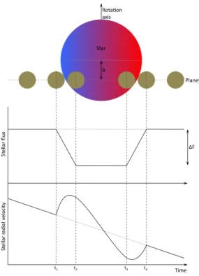
Figure 1.1: An illustration of the detectable changes that are caused by the transit of a star by an extra-solar planet. The points t₁, t₂, t₃, and t₄are known as the contact points, and mark the points at which the star enters/leaves the stellar disc, and the start/end of the period during which the planet is completely in front of the stellar disc. The impact parameter, b, is the shortest distance between the centre of the star and the transit chord. The change in stellar flux is defined as∆F , and causes a detectable photometric signature.

A spectroscopic signature is also produced, and is visible in the stellar radial velocity curve. This arises owing to the occultation by the planet of the blue-shifted and red-shifted stellar limbs, which affects the radial velocity measurement.

to the same point in its orbit, and thus the orbital period can be determined if multiple transits are detected. Knowledge of the period then enables the orbital separation of the planet from its host star to be determined using Kepler’s third law.

(30)

and stellar radii, and varies with impact parameter (and observational wavelength) owing to limb darkening. Accurately accounting for the effect of limb darkening on the transit lightcurve remains a significant problem; no single model has proven most successful at char-acterising limb-darkening, as the coefficients that are used depend on the wavelength being used (the effect becomes stronger as the wavelength decreases), and require data with a high signal-to-noise ratio (SNR) if they are to accurately replicate the observed variation in transit depth. Nevertheless, there are some models which are widely used throughout the literature (e.g. Claret, 2000, 2003, 2004a).

Until relatively recently transit searches were exclusively carried out from the ground by wide-angle survey telescopes such as SuperWASP (Pollacco et al., 2006) and HATnet (Bakos et al., 2002). However the vagaries of observing from the ground implicitly limit the SNR and precision that are achievable by such instruments. In 2006 the COROT (COnvection, ROtation and planetary Transits) satellite (Bordé et al., 2003) was launched, followed in 2009 by NASA’s Kepler mission (Borucki et al., 2008), which was designed specifically to search for transiting terrestrial planets.

1.2.1 The WASP project

The Wide Angle Search for Planets (WASP) project is, to date, the most successful ground-based transiting planet survey. It has discovered more than 100 planets; the majority of these are similar in mass and radius to Jupiter, but the survey has also found several Saturn and Neptune size objects, as well as one or two brown dwarfs.

WASP uses two survey telescopes to carry out its initial scan for potential transit signa-tures: SuperWASP, on the Canary Islands, and WASP-S, in South Africa. Each consists of eight off-the-shelf camera lenses, and measures the flux from thousands of stars every night. These data are processed by an automatic search algorithm which identifies the most probable or-bital and physical solution for the system based on the available data (Collier Cameron et al., 2006, 2007).

(31)

[image:31.595.124.454.87.317.2]

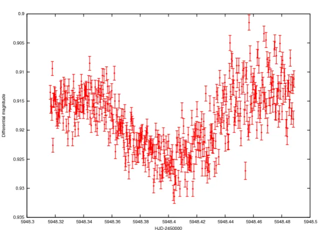
Figure 1.2: Photometric transit observations for the exoplanet WASP-93, obtained by the author using the James Gregory Telescope at the University of St Andrews Observatory.

and stellar radii (R_p/R_s), and of the stellar radius and orbital semi-major axis (R_s/a), as well as the impact parameterb. By using Kepler’s 3rd law it is then possible to determine the stellar density (ρ_s) and, if the stellar mass is known, the stellar radius (R_s). For WASP candidates an estimate of the stellar mass is made using the (J-K) colour of the target as listed in the 2MASS database (Skrutskie et al., 2006). Planetary and orbital parameters then follow, and enable a decision to be made regarding the plausibility of the transit being planetary in origin.

1.2.2 Candidate confirmation

(32)

Not all planet discoveries are able to be followed up. (Micro-lensing events, for exam-ple, are non-repeatable, but a great deal of care is taken to ensure that the detections are robust.) This is particularly a problem for Kepler as it pushes towards smaller and smaller planets. Kepler discoveries are too small, or require too much telescope time, for traditional follow-up to be viable. Thus the long list of Kepler ‘candidates’ as compared to their list of ‘planets’; many of the former are very strong candidate planets, but cannot be confirmed at this time using the instruments that are available. The Kepler science team have managed to create some very interesting, innovative methods for discovery confirmation (for example the BLENDER routine, Torres et al. 2011), but for some of their candidates even these are unable to completely rule out all false-positive scenarios.

SuperWASP follow-up

During my PhD I have been heavily involved in the follow-up program of the WASP project, and have carried out both spectroscopic and photometric observations of extra-solar planet candidates.

The main contribution that I made to the follow-up program was through photometric candidate confirmation using the James Gregory Telescope at the University of St Andrews observatory. Figure 1.2 shows an example of photometric transit observations that I made as part of this program. Over the course of more than 70 nights I observed more than 45 candidate transiting systems; to date 5 have been confirmed as planetary in nature, while several others remain strong candidates but require spectroscopic follow-up observations to fully cement their planetary status.

I also made contributions to the radial-velocity program through observing runs at the Observatoire de Haute-Provence (OHP) and at ESO’s La Silla site. My nine night run at the OHP made use of the SOPHIE spectrograph, and directly led to confirmation of at least one WASP planet. My two runs at La Silla were for ten nights and eight nights, using the HARPS instrument.

1.3 What can transits tell us?

(33)

radial velocity follow-up is a powerful one that can reveal a whole host of useful information.

1.3.1 Physical properties

One of the most important properties of a transiting system is the limited range of possible system geometries that is imposed - since transits are visible the inclination of the system must be well constrained. It is this which allows us, in combination with the aforementioned follow-up observations, to place excellent limits on a planet’s mass and radius. This in turn provides us with the information needed to determine planets’ bulk compositions. A remarkable range of exoplanetary structures have been deduced, from gas giants similar to Jupiter or Saturn, to planets with greatly extended atmospheres, massive cores, or a significant proportion of their mass in the form of ices. The existence of ‘ocean planets’, which would have the majority of their bulk composed of water, has also been postulated (Léger et al., 2004), and some may have been discovered (Kaltenegger et al., 2013). Thanks to the contribution of the Kepler satellite, we have even found planets with masses down to a few times that of the Earth, including bodies which appear to be rocky in nature (e.g. Fressin et al., 2012; Barclay et al., 2013).

The planetary interior models used to determine these compositions are commonly de-rived from models of the Solar system planets, for which the composition is well known, with the details of each layer varying from planet to planet depending on their observed proper-ties (Baraffe et al., 2010). The majority of the Jovian exoplanets appear to follow a similar structure: outer envelopes of hydrogen and helium, with some heavier metal enrichment, and a core of heavy elements such as carbon, nitrogen, and oxygen in their volatile, molecular forms. Some studies (e.g. Sudarsky et al., 2000) have also postulated the presence of silicate and iron cloud decks, and it is thought that phase transitions may exist within planetary inte-riors, particularly where hydrogen and helium are present (Chabrier, 2009), which can create challenges for theoretical models of planetary structure.

(34)

Figure 1.3: Left: Planetary mass as a function of orbital semi-major axis. Right: Planetary radius as a function of orbital semi-major axis. In both plots the axes use logarithmic scales. Plots are taken from

www.exoplanet.eu

In both plots it is apparent that there are certain regions of parameter space which are more densely populated than others. Planets found inside the red region in the left-hand panel were generally discovered by wide, shallow, ground-based transit searches. The planet marked in blue is WASP-19, one of the systems which will be discussed in Chapter 4.

The advent of the Kepler space mission has pushed the limit of the distribution towards the lower left corner of both plots, whilst micro-lensing experiments probe the parameter space at the opposite corner of the figures.

2002). If the transit is observed to be deeper in a particularly bandpass, then that implies that the species which corresponds to that bandpass is present in the planet’s atmosphere (Charbonneau et al., 2002). Observations at different wavelengths allow the presence, or otherwise, of different chemical species to be deduced. Once a set of measurements for a given planet has been built up they can be compared to model atmospheric spectra to gain further information about the planet. These measurements are very difficult to carry out, and can be subject to controversy (e.g. Swain et al., 2009; Gibson et al., 2011), but there is still great excitement about their potential (Barstow et al., 2013).

1.3.2 Orbital parameters

(35)

It is therefore not surprising that a large number of such planets have been found by transit search programs. Many of them have masses and radii similar to Jupiter, but orbit their host stars with semi-major axes less than or equal to that of Mercury (see the area marked in red in Figure 1.3). Known as ‘hot Jupiters’, they have been discovered down to very small semi-major axes (e.g. Hellier et al., 2009; Hebb et al., 2010; Sasselov, 2003). A large fraction of the known hot Jupiters have been found by wide, shallow, ground-based transit searches, of which they constitute the main harvest. Whilst such surveys were dominant, it was hot Jupiters which were the most common form of known planet. But they are poorly represented in the Kepler sample, indicating that they are actually rather rare.

Current theories of planet formation are unable to produce hot Jupiters in situ, as the protoplanetary disc close-in to the star would be too hot for sufficiently massive cores to form, preventing the planet from accumulating sufficient gas (Melo et al., 2006). The com-monly held view is therefore that hot Jupiters formed further out from the star before moving inwards under the influence of some migration mechanism. There are several competing hy-potheses for what this mechanism might be, but conclusive evidence for one or more of them being dominant has yet to emerge.

In the near future it may be possible to distinguish between them using the spectroscopic transit signature (see Figure 1.1). This phenomenon provides information on the alignment of the planetary orbit to the rotation of the host star, and will be discussed further in Chapters 5 and 6. When the angle between the orbital and rotation axes is measured, it is used to classify the system as ‘aligned’ or ‘misaligned’ according to some pre-existing criterion (e.g. Winn et al., 2010a).

Observations by the Kepler satellite have revealed a fascinating variety in the architecture of planetary systems. Examples with almost every conceivable combination of single and multiple planets, both gaseous and terrestrial, and with a wide range of orbital distances, eccentricities, and periods have been found. The possibilities seem to be endless.

1.4 Star-planet interactions

(36)

system’s evolution.

Examination of the minimum orbital separation for hot Jupiters reveals that the inner limit of the distribution is at approximately twice the Roche limit, the orbital separation at which a planet fills its Roche lobe and is tidally disrupted (Ford & Rasio, 2006). This agrees with models of the distribution expected if the formation process leaves hot Jupiters on highly eccentric orbits that are later circularised (Ford & Rasio, 2006; Rice et al., 2008). It has also been suggested that the limit results from tidal forces, or from extreme irradiation-induced mass loss that causes planets to ‘evaporate’ before they reach the Roche limit (Ford & Rasio, 2006). It is likely that the true explanation is some combination of all of these explanations, and of others that have yet to be determined.

1.4.1 Magnetic fields: chromospheric spots

Very close in hot Jupiters might interact with a star through their respective magnetic fields. The stellar coronal field and the planet’s magnetosphere can interact to produce bright chro-mospheric spots on the surface of the star. In the Solar system this has been observed in the Jupiter-Io system, but the situation in hot Jupiter systems is analogous, and it has been suggested that such spots might explain modulation in the chromospheric activity of some extra-solar planets.

The chromospheric spots have been claimed to rotate in phase with the orbit of the planet, rather than the rotation of the star, suggesting that they are induced by the planet rather than resulting from a process within the star itself (Shkolnik et al., 2003, 2005). However, the spots show an offset in phase compared to the longitude of the planet, with the magnitude of the offset varying from system to system (Shkolnik et al., 2008). Moreover the modulation phenomenon is not consistently observed, and in some cases the level of stellar activity was found to be higher outside of the observed events than during them.

Several models have been proposed for chromospheric signature generation, including Alfven waves and magnetic reconnection. Currently the latter seem to be provide the best explanation, through energy dissipation in loops connecting the magnetic fields of the two bodies (Lanza,priv. comm.). The available data are limited and few in number though, and whilst it is clear that something is occurring, the root cause remains uncertain.

(37)

indicators. A small number of very-hot Jupiter hosts have been found to be under-active compared to other stars of similar spectral type, and it has been posited that a tail of material, produced through atmospheric blow-off, might be the cause. (Fossati et al., 2013)

1.4.2 Radiation: atmospheric blow-off

One of the most obvious ways in which stars and planets can interact is through the star’s radiation. The stellar wind radiates outwards from the star, and can interact with the planet’s magnetosphere. Examples of this interaction are abundant in our own Solar system (e.g. the Aurora Borealis), but the more extreme conditions that are found in many exoplanet systems produce correspondingly more impressive results.

The mass and radius of a hot Jupiter can be strongly affected by the properties of its host’s stellar wind, with the X-ray emission derived wind in particular having a large impact through irradiation of the planet. The incident X-ray flux slowly strips the atmosphere away from the planet by exciting molecules such that their velocities are greater than the planet’s escape velocity. In principle this is easily detectable, as the stripping of the atmosphere will produce an observably extended radius, which in turn results in a deeper transit. This can easily be misconstrued as simply a bigger planet, with a correspondingly lower density, but in the case of atmospheric stripping the depth of the transit will be wavelength dependent.

Such an effect has been observed for the exoplanet HD209458 (Vidal-Madjar et al., 2003), which has been confirmed to be undergoing atmospheric loss owing to stellar irradiation (Ehrenreich et al., 2008, and references therein). It has been suggested that the planet WASP-12 b might be undergoing similar irradiation-induced mass loss (Fossati et al., 2013), but alternative suggestions for the unusual transit profile have also been put forward (Vidotto et al., 2010).

Other examples of atmospheric blow-off can be found in the literature.

1.4.3 Gravitation: tides

(38)

in Chapter 3, and my own work on this area is the subject of Chapter 4.

1.5 Conclusion

As I alluded to at the start of the Chapter, it is an interesting and exciting time to be working in the field of exoplanetary science. New discoveries are being made, new avenues of research opened up, and new ideas put forward and tested every day. So much is in flux as our knowl-edge of planets outside of the Solar system continues to evolve. We are gradually learning that dynamical processes can shape planetary systems in chaotic and unpredictable ways, leading to a bewildering variety of outcomes, some of which are catastrophic. By studying the evolu-tionary paths to the various planetary end products, we can also learn about the importance of catastrophic dynamical events such as the Late Heavy Bombardment in the history of our own Solar system, and in the assembly of the one habitable planet that we know of.

In this thesis I will investigate one of the most consequential of these processes: the tidal interactions between a planet and its host star. Using hot Jupiter systems, I will show that their influence on the geography and history of planetary systems is marked. Figure 1.3 offers clues that tides are gradually eroding the inner boundary of the planet distribution, but how severe is this erosion? When does it happen? How long does it take? To answer these questions, we must first study the host stars to establish ages for systems which offer an insight into tidal processes. Only once these have been determined can we ascertain the role of tides in the evolution of many of the physical and orbital parameters of extra-solar planetary systems.

Nota Bene

(39)

(40)

2

Age determination for exoplanet host stars

Facets of the stellar model fitting work presented in this Chapter have appeared in a

range of WASP discovery publications. All work discussed is my own.

Stellar ages are generally poorly understood, and poorly characterised. The root of the prob-lem is that stellar age determination is a notoriously difficult exercise, owing to our incomplete knowledge regarding the intricacies of stellar structure. Yet they are becoming increasingly important as a stepping stone to a better understanding of planetary systems. As the focus of the exoplanet community shifts from discovery to characterisation, the evolution of exoplanet systems has become a hot topic. In order to fully comprehend the timescales involved in such processes as planetary formation and destruction, orbital migration and circularisation, and intra-system dynamical interactions, it is vital that we are able to accurately assess the ages of exoplanet host stars.

(41)

asteroseismology; lithium abundance; stellar rotation period, and Galactic space velocity are just some of the examples. Yet on closer inspection the physical situation underlying this assortment of techniques is both more simple and more complex than it might appear on the surface, and many of the plethora of metrics and parameters can be traced back to the same physical underpinnings: stellar rotation, and convective zone depth. Does this lead to broad agreement between the different methods, or do they produce a broad span of estimates? Are some of the methods more suitable, or reliable, in a given context than others? Is that even a valid question to ask?

In this Chapter I will address these questions for two age estimation methods, stellar model fitting and gyrochronology. I will apply these methods to a large sample of planetary systems, and look at the overall properties of the set of results that I obtain. My sample consists of 137 planetary and brown dwarf systems. The majority (97) of these are the host stars for the complete set of sub-stellar companions discovered by the WASP project as of 2013 March 1st, including many which have yet to be published but for which I was able to obtain data through my collaborators. The remainder are systems with measured spin-orbit alignment, as listed in the Holt-Rossiter-McLaughlin database of René Heller1 as of 2013 January 10th.

2.1 The importance of spectral type

The temperature of a star determines its spectrum, from which both its broad-band colours and spectral type can be found, thus determining many of its physical properties. Mass, radius, and temperature, not to mention the very structure of the star, are governed by the spectral type. The last of these has particularly far-reaching consequences. Is the star fully convective, or does it have a radiative core? How large and massive is the surface convective zone com-pared to the global mass and radius of the star? These points plays a role in many observable quantities, including tidal strength (Zahn, 1977), the properties of the stellar magnetic field and wind, stellar activity (Noyes et al., 1984a), and the mixing processes that govern stellar abundances.

The effects of spectral type on the physical properties of a star can be characterised through the use of theoretical models of stellar evolution. In fact the global properties of a star are entirely determined by its mass, age, rotation, and chemical composition (Vogt,

1

(42)

1926; Russell, 1927). Many different sets of models are available for determining these prop-erties, but they are all predicated on the same basic idea. A choice of input physics is made, and a set of initial parameters chosen. These parameters are then evolved according to the chosen physical principles, and the evolution of the stellar parameters recorded at each time step. This is repeated for a large number of initial parameter sets to build up a grid results such that the parameters of a star of a particular spectral type at a particular age can be found.

Although different sets of stellar models may appear to be very different, Southworth (2009) noted that they are often based on the same, or similar, physical underpinnings as each other, differing only in their implementation of said physics.

2.1.1 Stellar model fitting

Stellar model fitting (also known as isochrone fitting) as a means of stellar age estimation is fairly ubiquitous. This method’s widespread use probably originates from its adaptability, and from the relative simplicity of its implementation. At its core the method simply compares measured stellar parameters to theoretical models appropriate for the metallicity,[M/H], of the star being examined. The underlying physics, however, can be complex, as these models require detailed knowledge (or assumptions) of stellar structure. For some other methods, such as asteroseismology, this is not the case.

(43)

Traditionally, the effective temperature, Teff was measured from high resolution spectra

and, in conjunction with the absolute stellar magnitude Mv, interpolated through the

theo-retical data to obtain estimates of the stellar radius, stellar mass, and stellar age for the star (e.g. Edvardsson et al., 1993; Lachaume et al., 1999). For cases in which the distance to the object is poorly known, some studies replaced Mvwith the stellar surface gravity, log(gs)

(e.g. Konacki et al., 2005; Bouchy et al., 2005). This can often be difficult to determine pre-cisely however, even with very high quality spectra, but transiting planets offer an alternative choice of parameter space. The geometry of a transit means that the stellar density can be constrained to high precision using high signal-to-noise transit photometry (Seager & Mallén-Ornelas, 2003). Modern attempts at isochronal analysis in exoplanetary studies therefore tend to use the parameter space of[T_eff,(ρ_s/ρ)−1/3](Sozzetti et al., 2007).

Limitations

As previously mentioned, one of advantages of the stellar model fitting procedure is its sim-plicity. Very little data is required, and it is easily extendable through variation in the choice of stellar models used. The method is also applicable to a broad range of spectral types, in principal. But in reality, there are regions of parameter space in which it is difficult to obtain useful results.

In particular, it can be hard to find the ages of stars with spectral type later than mid-late G. These stars have nuclear burning timescales that are longer than the age of the Galactic disc. Such stars evolve very slowly, and have effective temperatures such that they fall into regions of parameter space in which theoretical isochrones are closely spaced (see Figure 2.1). This makes determining accurate and precise ages very difficult, even if the physical parameters of the star are well constrained, as even small error bars in Teff andρ−1/3 can cover a wide

range of ages. As far as exoplanet hosts are concerned, Triaud (2011) suggested that stars with M_s <1.2M were particularly problematic. The complex shapes of isochrones, particularly near the main-sequence (MS) turn-off, can also present issues, and interpolating through them is not always a valid approach owing to their non-uniform spacing (Soderblom, 2010). In addition, the less pronounced radius increase (and therefore density decrease) during the MS lifetime,τ_MS, of low mass stars compared to their more massive relations has an impact on age estimates.

(44)

stellar models cover, and of the format of those models. The minimum and maximum stellar mass are rarely problematic given the propensity for the host stars of transiting exoplanets to be of F or G spectral type and therefore broadly similar to the Sun (Bentley e.g. 2010, for WASP targets; Batalha et al. e.g. 2010, for Kepler targets). However the lower and upper limits on the stellarage are much more likely to come into play, and in some sets of stellar models the maximum isochrone age is greater than the currently accepted age of the Universe! In addition, most stellar model formulations struggle with very young systems, as close to the zero-age MS the isochrones compact, leading to similar problems as experienced with K- and M-dwarfs.

The choice of stellar model being used can have a large impact on the derived properties of planetary systems, particularly through the introduction of systematic errors (Southworth, 2009). This suggests that multiple sets of stellar models should be used if at all possible, in preference to relying on a single formulation.

2.2 Stellar rotation as a fundamental parameter

Stellar rotation plays a central role in governing many of emergent properties of the stars that we observe. Several of the metrics that are used for determining stellar age can be traced back to stellar rotation, and in some sense are merely acting as its proxies.

Research linking stellar rotation to activity, for example, has a long history. Vaughan et al. (1981) noted that many ‘cool’ stars appeared to exhibit quasi-periodic variation in their chromospheric activity level, as measured using emission in the Ca II H and K spectral lines. This was followed up by Noyes et al. (1984a,b), who found that the period of the activity cycle could be linked to the rotation period through the convective turnover time. They also found that, for slowly rotating stars, there was an additional dependence on stellar structure as parametrized by spectral type. These results are not surprising, as stellar activity is known to be correlated with the surface magnetic field, which is influenced by rotation (via convection within the star as a result of the stellar dynamo) and spectral type. The Noyes et al. equation,

P_cyc_∝P_rot(1.25±0.5) (2.1)

(45)

In light of this relationship, stellar activity is often used as a proxy for stellar age (e.g. Soderblom et al., 1991; Donahue, 1993; Mamajek & Hillenbrand, 2008), although many for-mulations provide implausible ages for both very active and very inactive stars (Mamajek & Hillenbrand, 2008). In this way it is possible to indirectly use stellar rotation as a proxy for age. But it is also possible to use the rotation of a star to directly infer its age.

Although it had been suggested by several authors that stellar rotation could change over time (Parker, 1958; Schatzman, 1962; Kraft, 1967), the link between rotation and age was first characterised by Skumanich (1972) in the well-known Skumanich law,

Prot∝tζ, (2.2)

which relates stellar rotation period to time. Since that landmark paper a substantial body of work has built up that looks at the relationship between stellar rotation and age (see Barnes & Kim (2010) for an excellent summary of the history of stellar rotation studies), and the Skumanich law continues to provide a solid foundation for such work.

2.2.1 The Skumanich exponent,

ζ

Skumanich (1972) suggested a value for the Skumanich exponent ofζ =0.5, but more re-cent work has shown that no single value of the exponent is able to correctly reproduce the observed rotational period distributions for all stellar populations. For example, the period distributions of stars in open clusters are not adequately described using ζ=0.5, and a dis-continuity in the relationship betweenProtand spectral type has been observed in the Hyades,

Praesepe, and M37 clusters. In the Hyades this break appears at spectral types K8-M2 (Scholz & Eislöffel, 2007), in Praesepe it seems to occur at around M1 spectral type (Covey et al., 2011), or 0.3−0.65M (Delorme et al., 2011a; Scholz et al., 2011), and in M37 it is found at around 0.8M(Hartman et al., 2009). It seems likely that these breaks arise as a result of the aforementioned difference in structure between very low mass stars and earlier spectral types, although the loss of the radiative core happens at lower stellar mass than the break in rotational period.

It is possible to determine a value forζusing stellar cluster data. By plotting stellar (B-V) colour as a function of rotation period, Prot, and fitting a curve to the data, the period-colour

(46)

Hyades (Radick et al., 1987) and Pleiades (Hartman et al., 2010) clusters, and in combination with their respective ages this allows a value of ζ to be calculated. This period-colour-age relation can then be calibrated using data from other stellar clusters. The Coma-Berenices cluster, for example, has also been studied (Collier Cameron et al., 2009), and an almost linear relationship, similar to that for F, G, and K stars in the Hyades, found between (J-K) colour andProt. Using the Hyades to calibrate their observations, Collier Cameron et al. found

only a small deviation from the standard Skumanich exponent, obtaining ζ = 0.56. This value has since been used by Delorme et al. (2011b) to analyse Praesepe in a similar manner. These, and similar studies for other clusters such as NGC2301 (Sukhbold & Howell, 2009), M34 (James et al., 2010), NGC6811 (Meibom et al., 2011), and M35 (Meibom et al., 2009), show that although stars of any given spectral type can be born with disparate rotation rates, theProt distribution becomes narrower over time. This occurs owing to the fact that magnetic

braking affects rapidly rotating stars more strongly than slower rotators, so that the rate of spin down increases with increasing initial rotation rate.

There is also evidence that the Skumanich exponent is not constant across the full colour range. A value ofζ=0.35 has been suggested for stars with 0.5®(J−K)®0.8 in Praesepe

(Agüeros et al., 2011), whilst a different study found that an exponential braking law,

Prot∝et/τ, (2.3)

with a mass-dependentτreproduces the data for very low mass stars (Scholz et al., 2011).

Whatever the exponent, or indeed the precise equation, the principle behind the Sku-manich law remains the same. The rotation of a star slows down as it ages. This fundamental stellar property arises owing to the action of magnetic braking on isolated stars (Weber & Davis, 1967)

2.2.2 Magnetic braking

(47)

Assuming a Weber-Davis model (Weber & Davis, 1967) for the stellar wind, then near the stellar surface the magnetic field lines are radial. The stellar wind must follow these field lines, and so the magnetic field exerts a torque on the wind. As the wind moves outward the magnetic field (and therefore the applied torque) weakens, and the particles that make up the stellar wind are free to travel along straight lines (when viewed in the initial frame of reference). The wind particles effectively drag the stellar magnetic field lines with them, forcing them into a spiral shape when viewed from above the rotation pole of the star. In the co-rotating frame of reference it is motion of the stellar wind that is radial close to the star; due to the reduced torque this particle outflow then curves backwards as the distance from the stellar surface increases, conserving angular momentum and slowing the rotation of the star (Reiners et al., 2009). Over the star’s main-sequence lifetime this causes the rotation period to gradually increase, such that a precise measurement of the period can, given knowledge of ζ, lead to an estimate of the stellar age through equation (2.2).

The strength of the magnetic braking torque is strongly dependent on the strength of the stellar magnetic field, which is determined by the interior structure of the star (Scholz & Eis-löffel, 2007). The size of the convective zone compared to the radiative core fundamentally affects the dynamo action that generates the magnetic field; whilst fully convective stars are capable of generating strong magnetic fields, the form of those fields is fundamentally differ-ent to that found in stars with both convective and radiative compondiffer-ents (Scholz & Eislöffel, 2007). It is also possible for the stellar dynamo to saturate at high rotation rates, restricting the strength of the stellar magnetic field and therefore stetting an upper limit on the rate of magnetic braking (Collier Cameron & Jianke, 1994). It is thought that for Sun like stars, this saturation occurs at approximately ten times the solar rotation rate (Soderblom, 1998).

2.2.3 Gyrochronology

(48)

distance to the star in question.

Calibrating with transiting planets

As well as being useful for stellar model fitting, planetary systems are also useful calibrators for gyrochronology. The radial velocity follow-up which is carried out as part of the confirmation process for most transiting planets (see Chapter 1, section 1.2.2) provides measurement of the projected rotation velocity,vsinI, of the star. This is often constrained to high precision, particularly for more rapidly rotating stars where the ambiguity of rotation as compared to macroturbulence effects is reduced, and can therefore be used to provide reasonably well-constrained rotation periods.

It is also sometimes possible to determine the rotation period from high-precision pho-tometric follow-up. For active stars, the presence of star spots in the transit chord leads to visible anomalies in the transit lightcurve. If the same starspot is present during consecutive transits, then its movement through the transit can provide measurement of the rotation pe-riod of the star (Silva-Valio, 2008; Dittmann et al., 2009; Sanchis-Ojeda et al., 2011). If the host star is particularly active then rotational modulation can be seen in the out-of-transit lightcurve (Alonso et al., 2008), and can be modelled to provide a measure of the rotation period. If sufficiently precise photometry is available, for example from the Kepler satellite, then this is nearly always possible unless the active-region lifetime is much shorter than the stelar rotation period (or the stars are particularly inactive).

These direct measurements are obviously preferable to an indirect calculation based on vsinI andRs.

Strengths and weaknesses

(49)

rotation period. For the other systems, the rotation period is inferred using

Prot=

2πR_s

vsinI sini. (2.4)

This is not an ideal situation; measurement errors onRsandvsinI can very quickly propagate

into large errors in the rotation period, whilst vsinI can be difficult to measure for slowly rotating stars. Furthermore, the sine function itself causes problems when determining the inclinationi, with sini=0.99_±0.01 allowing 79◦<i<90◦(Soderblom, 1985). Finally, Vican (2012) found that, for a sample of stars observed by the DEBRIS survey, gyrochronology ages calculated using directly measured P_rot and inferred P_rot differed by an average factor of 1.6 (see their figure 2). However, Soderblom (2010) claim that the use of vsinI is reasonable if stellar rotation is the dominant contribution to line broadening.

The use of derived rotation periods is thus far from perfect, but is necessary if a suitable sample size is to be reached. Using directly measured rotation periods is not a perfect solution either though, as differential rotation on the stellar surface can produce discrepancies between the measured value and the true equatorial rotation period (Soderblom, 2010).

One major problem with gyrochronology is that it is only applicable if the natural rota-tional evolution of the star is allowed to progress without any outside influence. There are several factors which can prevent this from happening. The most relevant in the context of this thesis are the torques that act on both the star and its close-in exoplanets as a result of tidal interactions (see Chapter 4). If the mass ratio and orbital semi-major axis are sufficiently small, then these torques may be strong enough to overwhelm the natural spin-down, at least for short periods of time, and either cause it to accelerate or slow down. If this, or some other outside influence is present and not acknowledged, then the calibration of the gyrochronology equations can be incorrect.

(50)

previously discussed. The exact position of the break was solidified when (Wolff et al., 1986) showed that stars with earlier spectral type than F8 show little-to-no relation between Prot

and stellar age. This is significantly earlier than the breaks in rotation period at M spectral types seen in young stellar clusters (and mentioned previously).

The applicability of gyrochronology to stars above this break is therefore non-existent, a fact which is sidestepped in Barnes (2007) by limiting the method to “solar-type (FGKM) stars”. In fact stars earlier than F8 are usually disregarded when modelling the spin-down rate of low mass stars (Stepien, 1988), and any study using gyrochronology should be wary of utilising it more broadly than this. It is worth noting though that the early spectral types at which gyrochronology breaks down are those for which stellar model fitting can provide strong age constraints, such that the two methods are nicely complementary.

2.3 Implementation

Given some of the problems discussed in sections 2.1.1 and 2.2.3, I made the decision to limit the parameter space in which I was working. I restricted myself to working only with those systems which fell between spectral types F7 and G9 (inclusive). This was carried out using the effective temperatures given in table B1 of Gray (2008), leading to limits of 6226 K_≤ T_eff _≤ 5273 K. This accounted for both the magnetic braking boundary problem and the K-dwarfτ_MS issue, whilst retaining the sweet spot for ground-based transit surveys. Applying these limits reduced my sample from its original size of 137 systems to only 73 systems.

2.3.1 Stellar model ages

There are generally two ways in which stellar models are presented: either evolutionary tracks with fixed mass and varying time, or isochrones of a fixed age with varying mass, although the latter are derived from the former. Evolutionary tracks are calculated covering a range of stellar masses, using variable time steps. The isochrones are then interpolated through the evolutionary tracks. Since the primary characteristic that I am trying to determine is stellar age, I choose to work with isochrones where they are available.

(51)

Figure 2.1: An illustration of the effect of my limited T_eff parameter space on the Yonsei-Yale stellar models. Left: The full set of stellar models, for ages from0.1Gyr to20Gyr. Right: The parameter space available after accounting for some of the factors discussed in sections 2.1.1 and 2.2.3. The region marked in red (bounded at T_eff =6226K) shows the region disallowed by consideration of the magnetic braking boundary, whilst the area in blue (bounded at T_eff=5273K) indicates those systems with predicted main-sequence lifetimes longer than the age of the Galactic disc.

I have chosen to use five sets of stellar models in my analysis. These are the Padova isochrones (Girardi et al., 2010; Marigo et al., 2008), the Yonsei-Yale (YY) isochrones (Demarque et al., 2004), the Teramo isochrones and evolutionary tracks (Pietrinferni et al., 2004), the Victoria-Regina (VRSS) isochrones and evolutionary tracks (VandenBerg et al., 2006), and isochrones from the Dartmouth Stellar Evolution database (DSEP; Dotter et al. 2008). Figure 2.2 illus-trates the subtle differences between the appearance of the different models.

The main difficulty of stellar model fitting is that it is an attempt to fit a single point to a three-dimensional ([Fe/H],Teff,(ρs/ρ)−1/3) parameter space in order to derive associated parameters (age and stellar mass, M_s/M). The problem can trivially be reduced to a two-dimensional one by considering only a single metallicity value at a time, which I achieve by neglecting the uncertainty in[Fe/H], but this does little to reduce the difficulty of the task.

There are many possible fitting procedures. The simplest is to merely take the closest isochrone as the age of the system, but this often provides only crude estimates and has an accuracy that is constrained by the ages for which isochrones have been provided. A more involved approach would be to find the two closest isochrones and interpolate between them. Other approaches include the Bayesian approach of Pont & Eyer (2004).