Modeling Wind Energy Using Copula

(1)

ISSN Print: 2333-9705

DOI: 10.4236/oalib.1104984 Nov. 30, 2018 1 Open Access Library Journal

Modeling Wind Energy Using Copula

Zuhair Bahraoui

1*

_{, Fatima Bahraoui}

2

_{, M. Amin Bahraoui}

3

1_{Department of Mathematics, ESTSB, University Chouaib Doukkali, El Jadida, Morocco}

2_{Laboratory of Heat Transfer and Energetic, Faculty of Sciences and Techniques, Tangier, Morocco} 3_{Department of Mathematics, Faculty of Science and Technology, Tangier, Morocco}

Abstract

In most studies related to wind energy, the quantity of the air density is con-sidered constant, but actually, we know that it is variable and depending on others natural factors. We present a new procedure to estimate the wind den-sity power energy by simulating the components of the air denden-sity. The pro-cedure uses the copula theory and demonstrates that the estimated power energy is higher if the air density is not constant.

Subject Areas

Applied Statistical Mathematics

Keywords

Weibull, Nonparametric Estimation, Copula, Wind Speed

1. Introduction

Understanding the relationship between the components of wind power is fun-damental to exploits wind energy, as well as the identification of suitable natural sites to perform the energy-efficient design and giving the economic rentability

[1]. This involves that estimating wind energy in eolian installations can be con-sidered as a challenge to predict the productive capacity energy. The most accu-rate formula to calculate the power in wind farms is to make use the wind den-sity power energy

( , ) 3 1

2 T P

P= ρ SV ₍₁₎

where ρ₍T P, ₎ is the air density. This term is dependent generally on the

temper-ature T, and the pressure P, both of which vary with height, see for example [2].

S represent the useful surface of the wind sensor and v is the wind speed. In most

How to cite this paper: Bahraoui, Z., Bahraoui, F. and Bahraoui, M.A. (2018) Modeling Wind Energy Using Copula. Open Access Library Journal, 5: e4984.

https://doi.org/10.4236/oalib.1104984

Received: October 13, 2018 Accepted: November 27, 2018 Published: November 30, 2018

This work is licensed under the Creative Commons Attribution International License (CC BY 4.0).

http://creativecommons.org/licenses/by/4.0/

(2)

DOI: 10.4236/oalib.1104984 2 Open Access Library Journal

studies, the air density is taken constant (for physical simplifications or for not having sufficient data), and it’s replacing with the standard air density, taking the average sea temperature 15˚C, and 1 atmospheric pressure that is 1.225 kg/m3_{. In}

this case, the relationship between the power and wind speed is reduced to a li-near function.

In this paper, we use the copula theory to handle the structure dependence beyond the linear correlation between the naturals variables: The wind speed, temperature, and pressure. The air density is considered not constant and the power should be affected by the dependence which is the idea of this research.

The term of copula was introduced by [3] in the multivariate analysis concept, but it was not until 1986 when [4] and [5] focused more light on this type of function, giving an application in the finance field and exploiting the proprieties of the Archimedean copula. Applications have been extended in all fields [6] and of course for naturals sample type variable. One of the most salient properties of copulas theory is that it is possible to separate independently the function of the dependence from the marginals distribution function ones [7]. We use the same principle to treat the components of the air density, i.e. estimating an adequate copula for the wind speed and temperature and from another side an adequate copula for the wind speed and pressure. The marginals distribution function can be estimated independently.

[8] with a pioneering works find a suitable parametric copula for wind speed variables and its direction. Recently there is an important study relating to the dependence function in renewable wind energy. For example, [9] examines another type of copulas families to handle the dependency between wind speed and their directions [10] utilize a pair copula (conditional dependence) to analyze the correlation between the winds farms, while [11] use the extremes value theory and copulas function to determines the correlation between wind turbines that compose the wind farm. Others [12] examine the dependence between wind power production and electricity prices.

The remainder of this article is organized as: Section 2 describes the parame-tric and non-parameparame-tric distribution function to estimate the marginals proba-bility distribution. The selected copulas used in the study are presented in Section 3. In Section 4 we explain a procedure to simulate wind speed density energy power. An application to real data is analyzed in the Section 5. Finally, we conclude.

2. Marginals under Study

Given X X1, 2, , Xn a n independent and identically distributed sample with a unknown distri-bution function (cdf) F and probability density function (pdf) f. A natural way to estimates the distribution function F, is to consider the empiri-cal distribution function

( ) 1 1

i

n

emp i X x

F I

n = ≤

(3)

where I₍X x_i≤₎ is the indicator function of a set I(X xi≤). The correction of this

approximation

( )

n₁ emp

( )

F x F x

n =

+

₍₃₎

is considered in the empirical estimation because using directly (2) to estimate the copula function can cause the boundary problems. That is the copula distribu-tion funcdistribu-tion implanted to identify the dependence structure may not integrate one, for a discussion one can consult [13]. This transformation is closed to the uniform distribution and its similar to the so-called the pseudo-observation in-troduced by [4]. The second nonparametric approximation is using the classical kernel estimator (CKE) [14]

( )

1 ₁

ˆ n _i

i

x X

F x K

n = h

−

 

= _ _

 

∑

(4)

where K x

( )

=

_∫

_−∞x k t t

( )

d is some known kernel distribution function [14], like Epanechnikov or the Gaussian distribution function, the most used function used for this approximation, see for an efficiency comparison [15]. The parameter

h, that satisfied generally the condition h → 0 when n → ∞ , controlled the smoothness of the estimated function.

In this paper, we use the specific value, _h₌_3.572_σ_n1 3_{, where}

(

)

min sd R, 1.34

σ = and sd is the standard deviation of the sample and R is the sample interquartile range [14].

Finally, to fit wind speed distribution function we add a Weibull distribution function. Used generally in reliability field and failure times in physical systems, this distribution function is recommended by the International Standard IEC 61400-12 and is widely used in the context of eolian analysis of a wind speed, [1] [2].

The CDF of Weibull distribution is: , 1 e

k x k F λ λ   − _{ } = − _.

The pdf density function

1

, e 0

0 0

k

k k

k

k x _{si x}

f

si x

λ

λ λ λ

  − _{− }      _{  } _≥ =     < 

The mean and variance are, respectively:

( )

1 1

E X

k

λ  

= Γ +_ _

  and

( )

2 ₁ 2 2 ₁ 1

Var X

k k

λ     

= _Γ +_ _+ Γ _ + __

   

 

such that,

( )

1

0 e d

x t

x +∞t − − t

Γ =

_∫

is the Euler’s Gamma function. To estimate the parameters k,

λ

, exists various methods like the mean squared method or the moment method [16].

(4)

( )

in₁

(

i,

)

LV

θ

=

∏

₌ f X

θ

₍₅₎

whereconsist the set parameters to be estimated

3. Dependence e Model

To reveals the structure dependence between the pairs variable, (Wind speed, Temperature) and (Wind speed, Pressure), three parametric copula have been considered. A copula is a distribution function defined in the cubic interval

[ ]

2

0,1 with uniform marginal distribution functions U

[ ]

0,1 . If FX, and FYare

marginals distribution of variables bivariate

(

X Y,

)

, then from the Sklar theo-rem [3] for each bivariate distribution function H there exist a hidden cdf function called copula C such that H x y

( )

, =C F x F y

(

X

( )

, Y

( )

)

. For more proprieties on copula one can consult [18] and [19].

The first copula considered is the Gaussian copula which pertains to the implicit copulas. Copula associated with elliptical distribution and represent a symme-trical dependency. In addition, they become important whether we are analyzing the right or left tail of the distribution function.

3.1. Gaussian Copula

If we denote by ρ _{be the linear correlation coefficient between two random}

va-riables X and Y, the Gaussian copula with parameter ρ _{is expressed:}

( )

(

( )

)

(

)

( ) ( ) 1 1 1 1 2 2 2 2 , ,

1 _exp 2 _{d d}

2 1 2π 1

u v

C u v u v

st s t _{s t}

ρ ρ ρ ρ ρ − − − − Φ Φ −∞ −∞

= Φ Φ Φ

 ₋ ₋    =  −  − _ _

∫

where Φρ is the two-dimensional standard Normal distribution function with

correlation coefficient equal to ρ_{, and} Φ_{is the standard Normal one-di-}

mensional distribution.

3.2. Sarmanov Copula

The second copula family considered is the Sarmanov copula. The range of the subfamilies is infinite due to its way of constructing a copula. One can find a special sub-copula associated to each marginal distribution function. Let

(

X Y,

)

be a bivariate random vector with marginal probability distribution functions (pdfs) fX and fY. Also, let ψ1 and ψ2 two bounded non-constant

func-tion such that:

( ) ( )

1 d 0

X

f t ψ t t

+∞

∞ =

∫

, f tY

( ) ( )

ψ2 t td 0

+∞

∞ =

∫

The joint bivariate pdf introduced by [20] is defined as:

( )

, X

( ) ( )

Y

(

1 1

( ) ( )

2

)

h x y = f x f y +

ηψ

x

ψ

y

and the associated copula distribution function is:

( )

(

1

( )

)

(

1

( )

)

1 2

0 0

, u v X Y d d

C u v ₌uv₊η ψ F − t ψ F − s t s

(5)

The density is:

( )

(

1

( )

)

(

1

( )

)

1 2

, 1 X Y

c u v _{= +}

ηψ

F − u

ψ

F− v ₍₇₎

where FX and FY are the cumulative distribution functions (cdf’s) of X and

Y, respectively. Parameter η is a real number that satisfies the condition for all x

and y. 1+ηψ1

( ) ( )

xψ2 y ≥0 for all x and y.

Note that when = 0, X and Y are independent. This parameter is related to the correlation between X and Y (if it exists), [21] as:

(

)

1 2

, v v

Corr X Y η

σ σ

= ₍₈₎

where ψ1

( )

x = −x µX and ψ2

( )

x = −x µX and µX =E X

( )

and

( )

Y E Y

µ = (9) To give a range of the parameter η, we use the result giving by [13] when the support of fX and fY is not only belong in

[ ]

0,1 i.e. if the support of fX is contained in

[ ]

a b, and that of fY is contained in

[ ]

c d, where a, b, c and

d are finite real numbers, then:

(

)(

)

(

)(

)

(

)(

)

(

)(

)

₍

(

)(

₎₍

)

₎

₍

(

)(

₎₍

)

₎

max ,

min ,

X Y X Y

b a d c b a d c

a b b d

b a d c b a d c

b a d c

a d b c

µ µ µ µ

η

µ µ µ µ

 − − − − − −     ₋ ₋ ₋ ₋     − − − −  ≤ − − ≤ _ _ − − − −   (10)

3.3. Frank Copula

The ultimate copula is the Frank copula. This copula belongs to the so-called Archimedean copula, a family of dependence function used for here nice analyti-cal proprieties [5]. The main characteristic of Frank copula is that it does not present dependence in the extremes, but in the center. The parameter of depen-dence can take a large range, θ∈ −∞

(

,0

] [

∪ 0,+∞

)

, and then one can handle the negative dependence.

The Frank copula is defined as:

( )

, 1ln 1

(

1 e

)(

1 e

)

1 e

u v

C u v

θ θ

θ

_θ

θ

− − −  − −    = − −  −   .

4. Simulate the Wind Density Power Energy from a Copula

In this section, we describe a procedure to simulate the statistical behavior of the wind power density using a Monte Carlo method [22]. From (1) and dividing by the surface area we have:

( , ) 3 1 2

w T P

P = ρ V (11) This term can represent the kinetic energy per unit area related to the wind. Now employing the ideal gas law, one expressed the air density [1] a

(T p, ) 1.225 288.15_T _1013.3P

ρ = _  _{ } _

(6)

The wind power density (11) can be calculated in two way. The first way is con-sidering the air density ρ(T p, ) constant. In this case the mean power produced

until an observation z is:

( )

( , )

_{( )}

3

0

2 d

z T p w

AP z =ρ

_∫

f v v v (13) where f is the (pdf) of the wind speed. When the value z→ ∞ we have the av-erage of the power energy. The second case if the air density ρ(T P, ), is not

con-stant. For n registration of the data ρ(T p, )=

(

ρ(T P1 1, ),ρ(T P2 2, ), ,… ρ(T Pn n, )

)

, the mean

wind power energy can be calculated until the observation zk.

( )

1 ( , ) 3

1

2 k k

n

w k i T P k

MP z =

∑

₌ ρ z (14) Now to simulate the wind power energy density we start by simulating the wind speed variable coupled with the temperature and the pressure.

The same procedure describes in [19] to generate a pair of copula is used. To generate a two-dimensional random variable we do serve the conditional distri-bution of the random vector

(

U V,

)

:

(

|

)

_u

( )

P V U U u≤ = =C v

where u

( )

lim _u ₀

(

,

)

( )

,

( )

,

C u u v C u v C u v

C v u u + ∆ → + ∆ − ∂ = = ∆ ∂ .

The following algorithm simulate the wind density power energy: 1) Start by fixing a copula C, of wind speed and temperature.

2) Generate two independent random variables u1 and z from a Uniform

dis-tribution U

( )

0,1

3) Set [ ]₁1

( )

2 u

u ₌C− z

, where [ ]₁1

u

C−

denotes aquasi-inverse of Cu1. The

qua-si-inverse is: [ ]

_{( )}

{

}

( )

{

}

1 1 1 1 1 1

inf | if 0

if 0,1

inf | if 1

u

u u

u

x C z z

C z C z

x C t z

− −  ≤ =  =_ ∈  ≤ = 

4) The desired first pair is

(

u u1, 2

)

where u2 is a uniform variable related to

the temperature variable.

5) Fixing the random variable u1, and considering now the copula of wind

speed and pressure, we repeated the procedure to give a pair

(

u u1, 3

)

, where u3 is

a uniform variable related to pressure variable. 6) Taking the inverse 1

( )

_, _{1, 2,3}

i

F u i− ₌ _{, of the marginal distribution function}

used in (3), (for the inverse method one can consult [22]), the pairs variable (Wind speed, temperature, pressure) coupled and conserving the same structure of the dependence in sample data.

7) Replacing this terms in (11).

5. Data and Result

(7)

collected in the region Hrarza, situated in the north Morocco kingdom. Near on the straits of Gibraltar and surrounded by two seas, the Mediterranean and the Atlantic, this region suffers a gusty wind. The annual mean wind speed exceeds 6 m/s. For comparison with another region of the kingdom, we can consult [23] in the north of Morrocan. The Hrarza station covers the registration at the begin-ning of 2000. We use only the last years of the registration covering 365-day maximal wind speed and their correspondent temperature and pressure.

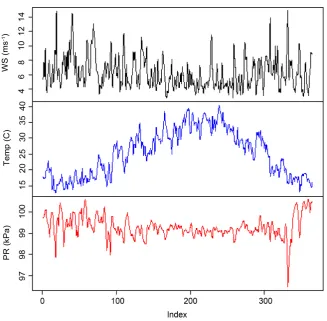
The first lecture of the graphical behavior of this variable Figure 1 is that the temperature variables are more predictable than the wind speed and the pres-sure. Probably due to the seasonal comportment. In Table 1 we give the descrip-tive statistics of the data. A simple reading for wind speed variable indicates that the distribution can be right skewness. The Jarque-Bera test of normality indi-cates that either variable is distributed Normally.

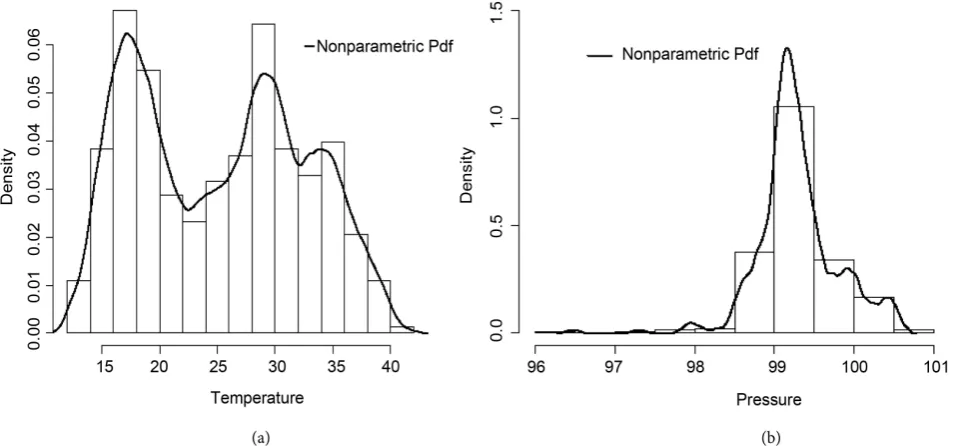
As we noted in Section 2 the marginal adjustment is resumed in Figure 2 and

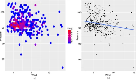
[image:7.595.210.538.386.707.2]

Figure 3. For the temperature and the pressure variables we have used the non-parametric estimation and for the wind speed, we have added the Weibull ad-justment. We note that the nonparametric estimation of the distribution gives a well fit for the three variables. To visualize the relationship between the pair (Wind speed, Temperature), (Wind speed, Pressure) we make use the regression

(8)

[image:8.595.59.537.73.305.2]

[image:8.595.60.537.336.559.2]

Figure 2. Distribution and density of wind speed. (a) Density of the wind speed; (b) CDF of the wind speed.

Figure 3. Density function of temperature and pressure. (a) Density of temperature; (b) Density of pressure.

Table 1. Descriptive statistics.

Average Std.Dev. Kurtosis Skewness Min Max JB Test

Wind Speed 6.263 2.233 1.463 1.117 2.730 14.870 2.200 × 10−16

Temperature 25.236 7.258 −1.255 0.100 12.870 40.410 5.522 × 10−16

Pressure 99.291 0.504 3.160 −0.227 96.468 100.578 2.200 × 10−16

[image:8.595.54.541.612.681.2]

(9)

[image:9.595.62.537.70.321.2]

Figure 4. Regression of wind speed and temperature. (a) Wind vs Temperature; (b) Regression line.

Figure 5. Regression of wind speed and pressure. (a) Wind vs pressure; (b) Regression line.

tool to identify the dependency structure between two variables confirm this relation, i.e. the point plotted is under the diagonal line wish indicate a negative dependency.

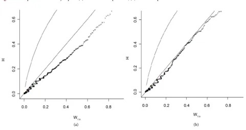
[image:9.595.63.532.355.632.2]

(10)

nonparametric estimation of copula density, Figure 6 & Figure 7 is also consi-dered. For an independent and identical variables

(

U V ii, i

)

, =1, 2, , n the

nonparametric estimation of copula density can be expressed:

( )

1 ₁ _* _*

ˆ , n _i _i

i

U u V v

c u v k k

n = h h

− −

   

= _ _{ } _

   

∑

, (15)

where k is the kernel pdf function and _h*_{is one of the smoothed parameters}

[image:10.595.67.538.197.696.2] [image:10.595.57.539.459.713.2]

for copula estimation [25].

Figure 6. Nonparametric density copula. (a) Wind and temperature; (b) Wind and pressure.

(11)

The package kdecopula [26] is used for R available language and environment for statistical computing and graphics. We observe that the associated copula for both, (Wind speed, Temperature) and (Wind speed, Pressure) doesn’t have ex-tremes dependance in the tail, but a large dependence in the center and tend to have symmetry form. The elliptical or an Archimedean copula can be a good fit for this type of dependence. In the Table 2 we summarize the estimate parame-ters for a proposed copula accompanied with the CIC criteria value to select the adequate statistics model. The method used in estimating the parameters of the copula is the inference from marginal, (IFM) introduced by [18]. This method consists firstly to estimate the distribution function of the marginal (CDF), and calculating the pair

(

F X F YˆX

( )

i , ˆX

( )

i

)

=

(

u v iˆ ˆi, i

)

, =1, 2, , n using (5). The

second stage is to minimize the log-likelihood function for a copula, that is

( )

in₁

(

ˆ ˆi, i

)

LVC

θ

=

∑

=C u vθ .

The (IFM) method has an advantage that they avoid the excess time optimiza-tion. Using a global estimation of the log-likelihood function considering both the marginals and a copula doesn’t guarantee the existence of the minimum,

[image:11.595.201.536.357.744.2]

[27].

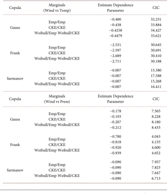
Table 2. Results of the fit of the copulas with nonparametric and semiparametric marginals.

Copula _{(Wind vs Temp)}Marginals Estimate Dependence _Parameter CIC

Gauss Emp/Emp CKE/CKE

Weibull/Emp Weibull/CKE −0.400 −0.438 −0.4258 −0.4479 32.251 33.884 34.427 35.621

Frank Emp/Emp CKE/CKE

Sarmanov Emp/Emp CKE/CKE Weibull/Emp Weibull/CKE −0.007 −0.007 −0.007 −0.007 15.380 17.588 15.268 16.411

Copula _{(Wind vs Press)}Marginals Estimate Dependence _Parameter CIC

Gauss Emp/Emp CKE/CKE

Frank Emp/Emp CKE/CKE

(12)

The CIC criteria give the best selection of copula among another copula. Like the Akaike information criterion [28], the CIC tools was introduced by [29] and it is designed when the dependence relation is considered. Analyzing the result of the Table 2 we can say that the Sarmanov copula gives the best fit for the de-pendency between wind speed and temperature and more specify using a Wei-bull distribution for wind speed and the empirical (CDF) for a temperature as marginals distribution function. In another hand, Frank copula give the best fit for the wind speed and Pressure and one can only use the empirical estimation for the marginals to give the best model.

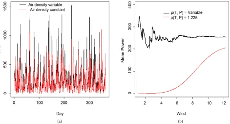
A simulation of daily energy is illustrated in Figure 8(a) using the procedure describes above in Section 4. We can generate then the best model that reflect the dependence structure of the variables coupling with their estimated marginal probability function. With the red lines, we have the wind density power (11) simulated when the air density is constant and with black lines if the air density is no constant. We note that there exists a notable difference between the two cases, and generally, the power energy is higher if the air density not constant. Finally, we plot, Figure 8(b), the mean of the wind density power energy simu-lated both in the case (13) and (14). The variation of mean in the case of the density is not constant is hight, stabilized at the total mean 252.181. Using the Weibull pdf function the mean of the density power energy is equal 214.8 less.

6. Conclusion

[image:12.595.66.538.438.691.2]

In this work, we have analyzed the statistical behavior of the wind energy in

(13)

north Morocco, from the point the view of the copula. Our objective is to give a most accurate simulation method for a density power energy in the eolian park. Fitting the marginal probability component of the wind density variable, we have noted that the nonparametric approach can give the best fit. To capture the nega-tive dependence between the variables we have used two type of copula. The Archimedean and the elliptical copula. We have incorporated Sarmanov copula wish has never been used in this type of data and giving a suitable model. The procedure introduced to simulate the wind density power energy can generalize to the other field related to renewable energies since the density of the air is al-ways present.

Conflicts of Interest

The authors declare that there is no conflict of interest regarding the publication of this paper and there has been no significant financial support for this work that could have influenced its outcome.

References

[1] Burton, T., Jenkins, N., Sharpe, D. and Bossanyi, E. (2001) Wind Energy Handbook. John Wiley and Sons, Inc., Chichester. https://doi.org/10.1002/0470846062

[2] Manwell, J., McGowan, J. and Rogers, A.L. (2010) Wind Energy Explained: Theory, Design. John Wiley and Sons.

[3] Sklar, A. (1959) Fonctions de répartition a´n dimensions et leurs marges. Publications de Institut de Statistique de l’université de Paris, 8, 229-231.

[4] Genest, C. and MacKay, J. (1986) The Joy of Copulas: Bivariate Distributions with Uniform Marginals. The American Statistician, 40, 280-283.

[5] Genest, C. (1987) Frank’s Family of Bivariate Distributions. Biometrika, 74, 549-555.

https://doi.org/10.1093/biomet/74.3.549

[6] McNeil, A.J., Frey, R. and Embrechts, P. (2005) Quantitative Risk Management: Concepts, Techniques, and Tools. Princeton University Press, Princeton.

[7] Genest, C. and Favre, A.C. (2007) Everything You Always Wanted to Know about Copula Modeling but Were Afraid to Ask. Journal of Hydrologic Engineering, 12, 347-368. https://doi.org/10.1061/(ASCE)1084-0699(2007)12:4(347)

[8] Coles, S. and Walshaw, D. (1994) Directional Modeling of Extreme Wind Speeds.

Applied Statistics, 43, 139-157. https://doi.org/10.2307/2986118

[9] Soukissiana, T.H. and Karathanasia, F.E. (2017) On the Selection of Bivariate Para-metric Models for Wind Data. Applied Energy, 188, 229-236.

https://doi.org/10.1016/j.apenergy.2016.11.097

[10] Cao, J. and Yan, Z. (2017) Probabilistic Optimal Power Flow Considering Depen-dences of, Wind Speed among Wind Farms by the Pair-Copula Method. Interna-tional of Electrical Power and Energy Systems, 84, 296-307.

https://doi.org/10.1016/j.ijepes.2016.06.008

[11] D’Amicoa, G., Petronib, F. and Pratticoc, F. (2015) Wind Speed Prediction for Wind Farm Applications by Extreme Value Theory and Copulas. Journal of Wind Engineering and Industrial Aerodynamics, 145, 229-236.

https://doi.org/10.1016/j.jweia.2015.06.018

(14)

Risk in Wind Power Trading: A Copula Approach. Energy Economics, 62, 139-154.

https://doi.org/10.1016/j.eneco.2016.11.023

[13] Bolancé, C., Bahraoui, Z. and Artis, M. (2014) Quantifying the Risk Using Copulate with Nonparametric Marginals. Insurance: Mathematics and Economics, 58, 46-56.

https://doi.org/10.1016/j.insmatheco.2014.06.008

[14] Silverman, B.W. (1986) Density Estimation for Statistics and Data Analysis. Chap-man and Hall, CRC Finance Series, London.

https://doi.org/10.1007/978-1-4899-3324-9

[15] Wand, M.P. and Jones, M.C. (1995) Kernel Smoothing. Chapman and Hall, Lon-don. https://doi.org/10.1007/978-1-4899-4493-1

[16] Pobockova, I. and Sedliackova, Z. (2014) Comparison of Four Methods for Esti-mating the Weibull Distribution Parameters. Applied Mathematical Sciences, 8, 4137-4149.https://doi.org/10.12988/ams.2014.45389

[17] Cohen, A.C. (1965) Maximum Likelihood Estimation in the Weibull Distribution Based on Complete and on Censored Samples. Technometrics, 7, 579-588. https://doi.org/10.1080/00401706.1965.10490300

[18] Joe, H. (1997) Multivariate Models and Dependence Concept. Chapman and Hall, London. https://doi.org/10.1201/b13150

[19] Nelsen, R.B. (2006) An Introduction to Copulas. 2nd Edition, Springer, Portland. [20] Sarmanov, O.V. (1966) Generalized Normal Correlation and Two-Dimensional

Fréchet. Soviet Mathematics. Doklady, 25, 1207-1222.

[21] Lee, M.L. (1996) Properties and Applications of the Sarmanov Family of Bivariate Distributions. Communications in Statistics-Theory and Methods, 25, 1207-1222. https://doi.org/10.1080/03610929608831759

[22] Devroye, L. (1986) Non-Uniform Random Variate Generation. Springer, New York. https://doi.org/10.1007/978-1-4613-8643-8

[23] Nfaoui, H., Buret, J.J. and Sayigh, A.A.M. (1998) Wind Characteristics and Wind Energy Potential in Morocco. Solar Energy, 63, 51-60.

[24] Genest, C. and Boies, J.C. (2003) Detecting Dependence with Kendall Plots. Journal of the American Statistical Association, 57, 275-284.

https://doi.org/10.1198/0003130032431

[25] Nagler, T. (2014) Kernel Methods for Vine Copula Estimation. Universi at Mun-chen, München.

[26] Nagler, T. (2017) Kdecopula: An R Package for the Kernel Estimation of Bivariate Copula Densities. https://CRAN.R-project.org/package=kdecopula

[27] Cherubini, U., Luciano, E. and Vecchiato, W. (2004) Copula Methods in Finance. Wiley, Chichester.https://doi.org/10.1002/9781118673331

[28] Akaike, H. (1973) Information Theory and an Extension of the Maximum Likelih-ood Principle. 2nd International Symposium on Information Theory, Tsahkadsor, 2-8 September 1971, 267-281.