Computation of Real Radical Ideals by Semidefinite Programming and Iterative Methods

(1)

Western University Western University

Scholarship@Western

Electronic Thesis and Dissertation Repository

10-20-2016 12:00 AM

Computation of Real Radical Ideals by Semidefinite Programming

and Iterative Methods

Fei Wang

The University of Western Ontario

Supervisor Greg Reid

The University of Western Ontario

Graduate Program in Applied Mathematics

A thesis submitted in partial fulfillment of the requirements for the degree in Doctor of Philosophy

Follow this and additional works at: https://ir.lib.uwo.ca/etd

Part of the Algebraic Geometry Commons, and the Other Applied Mathematics Commons

Recommended Citation Recommended Citation

Wang, Fei, "Computation of Real Radical Ideals by Semidefinite Programming and Iterative Methods" (2016). Electronic Thesis and Dissertation Repository. 4262.

https://ir.lib.uwo.ca/etd/4262

This Dissertation/Thesis is brought to you for free and open access by Scholarship@Western. It has been accepted for inclusion in Electronic Thesis and Dissertation Repository by an authorized administrator of

(2)

Systems of polynomial equations with approximate real coefficients arise frequently as models in applications in science and engineering. In the case of a system with finitely many real solutions (the 0 dimensional case), an equivalent system generates the so-called real rad-ical ideal of the system. In this case the equivalent real radrad-ical system has only real (i.e., no non-real) roots and no multiple roots. Such systems have obvious advantages in applications, including not having to deal with a potentially large number of non-physical complex roots, or with the ill-conditioning associated with roots with multiplicity. There is a corresponding, but more involved, description of the real radical for systems with real manifolds of solutions (the positive dimensional case) with corresponding advantages in applications.

The stable and practical computation of real radicals in the approximate case is an important open problem. Theoretical advances and corresponding implemented algorithms are made for this problem.

The approach of the thesis is to use semidefinite programming (SDP) methods from alge-braic geometry and also techniques originating in the geometry of differential equations. The problem of finding the real radical is re-formulated as an SDP problem. This approach in the 0 dimensional case was pioneered by Curto & Fialkow with breakthroughs in the 0 dimensional case by Lasserre and collaborators. In the positive dimensional case, important contributions have been made of Ma, Wang and Zhi. The real radical corresponds to a generic point lying on the intersection of boundary of the convex cone of positive semidefinite matrices and a linear affine space associated with the polynomial system.

As posed, this problem is not stable, since an arbitrarily small perturbation takes the point to an infeasible one outside the cone. A contribution of the thesis is to show how to apply facial reduction pioneered by Borwein and Wolkowicz to this problem. It is regularized by mapping the point to one which is strictly on the interior of another convex region, the minimal face of the cone. Then a strictly feasible point on the minimal face can be computed by accurate iterative methods such as the Douglas-Rachford method. Such a point corresponds to a generic point (max rank solution) of the SDP feasible problem. The regularization is done by solving the auxiliary problem which can be done again by iterative methods. This process is proved to be stable under some assumptions in this thesis as the max rank doesn’t change under suf-ficiently small perturbations. This well-posedness is also reflected in our examples, which are executed much more accurately than by methods based on interior point approaches.

For a given polynomial system, and an integer d > 0, results of Curto & Fialkow and Lasserre are generalized to give an algorithm for computing the real radical up to degree d. Using this truncated real radical as input to critical point methods can lead in many cases to validation of the real radical.

Keywords: SDP Optimization, Numerical Algebraic Geometry, Facial Reduction

(3)

Co-Authorship Statement

Chapters 2 -4 of this thesis consist of the following papers:

Chapter 2: Greg Reid, Fei Wang and Wenyuan Wu. A note on geometric involutive bases

for positive dimensional polynomial ideals and SDP methods. Proceedings of the 2014 Sym-posium on Symbolic-Numeric Computation, Pages 41-42. ACM, 2014.

Chapter 3: Greg Reid, Fei Wang, Henry Wolkowicz and Wenyuan Wu. Semidefinite

Pro-gramming and facial reduction for Systems of Polynomial Equations. Submitted toTheoretical Computer Science, arXiv:1504.00931, 2015.

Chapter 4: Fei Wang, Greg Reid and Henry Wolkowicz. Finding Maximum Rank Moment

Matrices by Facial Reduction and Douglas-Rachford Method. arXiv:1606.00491, 2016

The original draft for each of the above articles was prepared by the author and Greg Reid.

Subsequent revisions were performed by the author and Dr. Greg Reid. Development of

soft-ware, analytical and numerical work using MATLAB was performed by the author under

su-pervision of Dr. Greg Reid.

(4)

I would like to express my sincere gratitude to my advisor Prof. Greg Reid for the continuous

support of my Ph.D study and related research, for his patience, motivation, and immense

knowledge. His guidance helped me in all the time of research and writing of this thesis. I really

enjoy working with Greg who created an wonderful atmosphere which especially stimulates

my ability to work independently. I could not have imagined having a better advisor and

mentor for my Ph.D study. I also thank Greg for supporting me to attend many conferences

and workshops where I can present my work and meet many experts in my field of study, for

example, the wonderful to the SNC Shanghai conference to present my research. There are

also many other examples and I can’t list them all here.

Besides my advisor, I also owe a lot of gratitude to my supervisory committee members

Rob Corless and David Jeffrey. Before I started working in the field of real algebraic geometry, I worked with them on the Lambert W function. One of the work is published in ISSAC 14

Japan. Without their support, this could not be possible. Although my work on Lambert W

function is not the topic of this thesis, the experience gained by working with them has helped

me a lot in many aspects of my research. I also thank Rob Corless and David Jeffrey for many workshops they organized to create an inspiring environment inside the department. For

example, they organised the workshop ”20 years of Lambert W function” where I presented

my work and meet with people from many diverse and interesting research fields.

My sincere thanks goes to Prof. Henry Wolkowicz who is an expert in optimization. I

learned a lot of things about optimization from Henry. Henry introduced me to the idea of

facial reduction and Douglas-Rachford iteration which is very important in this thesis. I also

thank him for his many useful comments and references he sent to me which greatly widens

and deepens my knowledge about optimzation. My sincere thanks also goes to Wenyuan Wu

who is one of the coauthors of the paper for Chapter 2 in this thesis. The discussion with him

about the real radical and critical points gave lots of inspirations to me.

Last but not least, I would like to thank my family members and my girl friend for their

support, patience and understanding throughout my PhD study which I can’t describe in words.

(5)

List of Figures

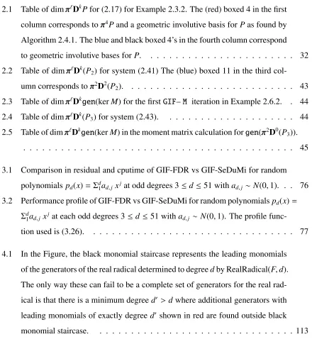
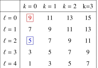
2.1 Table of dimπ`DkPfor (2.17) for Example 2.3.2. The (red) boxed 4 in the first column corresponds toπ4Pand a geometric involutive basis forPas found by Algorithm 2.4.1. The blue and black boxed 4’s in the fourth column correspond

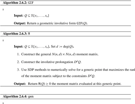
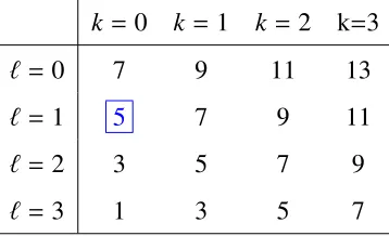
to geometric involutive bases forP. . . 32 2.2 Table of dimπ`Dk(P2) for system (2.41) The (blue) boxed 11 in the third

col-umn corresponds toπ2D2(P2). . . 43 2.3 Table of dimπ`Dkgen(kerM) for the firstGIF–M iteration in Example 2.6.2. . 44 2.4 Table of dimπ`Dk(P3) for system (2.43). . . 44 2.5 Table of dimπ`Dkgen(kerM) in the moment matrix calculation forgen(π2_D0₍_P

3)).

. . . 45

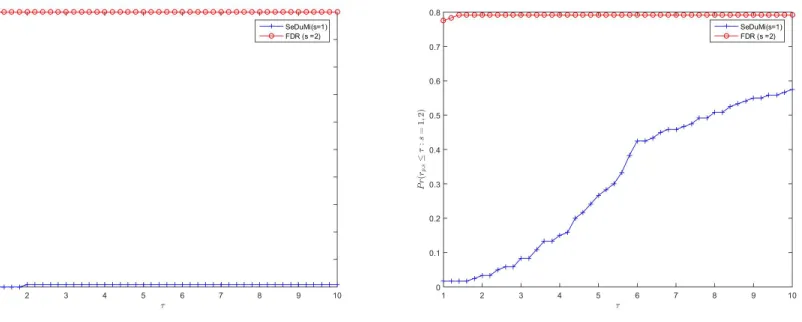
3.1 Comparison in residual and cputime of GIF-FDR vs GIF-SeDuMi for random

polynomialspd(x)= Σd₁ad,j xjat odd degrees 3≤d ≤51 withad,j ∼ N(0,1). . . 76

3.2 Performance profile of GIF-FDR vs GIF-SeDuMi for random polynomialspd(x)=

Σd

1ad,j xj at each odd degrees 3≤ d ≤51 with ad,j ∼ N(0,1). The profile

func-tion used is (3.26). . . 77

4.1 In the Figure, the black monomial staircase represents the leading monomials

of the generators of the real radical determined to degreedby RealRadical(F,d). The only way these can fail to be a complete set of generators for the real

rad-ical is that there is a minimum degreed0 > dwhere additional generators with leading monomials of exactly degreed0 shown in red are found outside black monomial staircase. . . 113

(10)

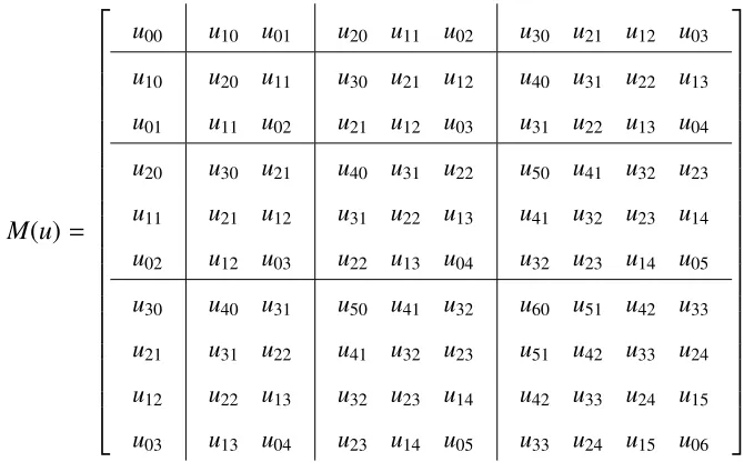
3.1 block partitioned bivariate moment matrix; submatrices have same degree . . . 66

3.2 Statistics for the application of GIF-FDR and GIF-SeDuMi: Ex 4.1-4.6 are 6

ex-amples in MWZ [37]; Cyl2d-Cyl5d are cylinder exex-amples; nnumber of variables; d

maximum polynomial degree; m number of polynomials; in columns 3,4, two en-tries (1,2) are included for the number of iterations and cpu-time if FDR is used twice

in the example; And we take the max value in the residual error columns 5 and 8;

(s(M),s( ˆM)) is sizes of moment matrixMand facially reduced matrix ˆM, resp.; col-umn 7 is the SVD tolerance for GIF and the residual error for the moment matrix using

the Interior Point calculation with SeDuMi, DNC - Did Not Converge; the Maple SVD

computations in GIF-FDR were executed with tolerance := 10−10 andDigits := 15,

resp. . . 82

4.1 Comparison between facial reduction and SeDuMi (1) All data is obtained by

using minimal number of facial reductions; Here: min (max) # FR means minimal

(maximum) number of facial reductions in our tests; rank(FR) means the size of the

problem after each facial reduction, the first one is the size of the original problem;

Singlty degree is the singularity degree of the SDP problem after the 1st facial

reduc-tion; Res(FR) is the residual of the final moment matrix using facial reduction and

DR iterations (Algorithm 4.3.1); Res(CVX) is the residual of the final moment matrix

using CVX(SeDuMi). . . 119

(11)

4.2 Comparison between facial reduction and SeDuMi (2) All data obtained here is

by using minimal number of facial reductions; max rank is the maximum rank of the

moment matrix; res each FR is the residual of solving the corresponding SDP problem

by DR after each facial reduction; # DR each FR is the number of DR iterations to solve

the corresponding SDP problem after each facial reduction; thres FR is the tolerance

to obtain the correct maximum rank using facial reductions (Algorithm 4.3.1); thres

CVX is the tolerance to obtain the correct maximum rank using CVX(SeDuMi); . . . 119

(12)

Appendix . . . 133

Appendix . . . 135

(13)

Chapter 1 Introduction

The thesis is aimed at developing theory and numerical algorithms for transforming a system of

polynomial equations with real coefficients into an equivalent potent system, called generating polynomial equations for the real radical of the system. Such real radical generating systems

enjoy potent properties: they are free of multiplicities which cause ill-conditioning in numerical

solution methods; in the case of finitely many solutions they have no non-real solutions; they

are free of sums of squares of polynomials. These and other advantages mean that the problem

of finding stable and efficient algorithms for the approximation of real radicals is an important open problem, which is the focus of much recent research [16, 20, 25, 6].

Systems of polynomial equations requiring analysis of their real solutions arise in many

ap-plications. For example, in mechanism design, the fixed distance between joints are expressed

naturally as quadratic equations in the joint coordinates [1]. In chemistry, equilibria of

chemi-cal reactions are naturally modelled as solutions of polynomial equations [26]. Biology yields

analogous systems and equilibria as real solutions of polynomial equations [22].

Historical high points in polynomial solving are the discovery of formulae for their exact

solution in terms of rational functions of the coefficients and radicals for the quadratic, cubic and quartic polynomials. Subsequently Galois and Abel famously showed that such formulae

do not exist for univariate polynomials of degree≥5. The mathematical study of such systems

and their solutions constitutesAlgebraic Geometry, one of the foundation areas of Mathemat-ics. Indeed only relatively few polynomials of higher degree are exactly solvable, with Galois

giving a criterion for such solvability. Since our focus is on general polynomial systems of

(14)

higher degree with approximate real coefficients, the methods developed in the thesis are nu-merical methods, rather than such exact methods.

This thesis is a multidisciplinary work between the areas of Computer Science, Algebraic

Geometry, Numerical Analysis, Convex Optimization, and methods originating in the

Geome-try of Partial Differential Equations. To help the reader understand the main ideas, in Section 1.1 we will introduce some elementary material on solutions of polynomial systems over the

real numbersRn and the complex numbersCn. In Section 1.2, we will introduce material on

ideals of polynomial systems over_Rand_C. The more complicated objects of radicals of these

ideals are also introduced in this section, together with simple examples. Section 1.3 will give

a simple introduction by examples to characterizing the real radical as the solution of a

semi-definite programming (SDP) problem involving a so-called moment matrix. Section 1.4 will

give some basic background about SDP problems, their primal and their dual forms, and facial

reduction. Section 1.5 gives a higher level view of the moment and moment matrix problem

and relevant results in the literature. Section 1.6 gives an outline of the contents of the thesis.

1.1 Real and complex solution sets (varieties) of systems of

polynomial equations

Throughout this thesis we consider systems of polynomial equations in variablesx=(x1,x2, . . .

,xn) which are either real (x ∈ Rn) or complex (x ∈ Cn), with coefficients which are usually

real or some times complex. Since we are not developing exact methods, we don’t consider the

case of exact (e.g. integer, rational, or modular) coefficients and focus on the case that mostly occurs in applications, that of real solutions of polynomials with real coefficients.

So we consider systems of polynomials in variablesx= (x1,x2, . . . ,xn):

p1(x)=0, . . . ,pk(x)=0 (1.1)

where usually the polynomials have real coefficients, that is each polynomial belongs to the polynomial ringR[x], or complex in which caseP={p1, . . . ,pk} ⊂C[x]. See [8], for definition

and discussion of polynomial rings. The solution sets (varieties) over _C and _R are naturally

(15)

1.1. Real and complex solution sets(varieties)of systems of polynomial equations 3

Definition 1.1.1 (Variety) Given P={p1, ...,pk} ⊂ R[x]where x= (x1, . . . ,xn)we define

VC(P) := {x∈C

n

: p1(x)= 0, . . . ,pk(x)=0} (1.2)

The solution set overR, or real variety, is defined as:

VR(P) := {x∈R

n

: p1(x)= 0, . . . ,pk(x)=0} (1.3)

Note that sometimes we will writeP(x)=0 for brevity, or evenp(x)= 0 instead ofp1(x1, . . . ,xn)=

0, . . . ,pk(x1, . . . ,xn) = 0. ObviouslyVR(P) ⊆ VC(P) and the geometry of the varieties can be

quite different as the following sum of squares example shows.

Example 1.1.1 Consider the single equation u2+v2 =0. Here x1= u,x2 =v. Then

VC(u

2₊_v2_{) :}₌ _{₍_u_,_v₎_∈

C2 :u2+v2 =0}={(+iv,v)∈C2} ∪ {(−iv,v)∈C2} (1.4)

VR(u

2₊

v2) := {(u,v)∈_R2 :u2+v2 =0}={(0,0)} (1.5) Here the complex variety is the union of two 1-dimensional manfolds (lines). The real variety

is 0-dimensional and consists of a point. To give the reader a brief taste of real radicals, the

complex radical for the above example has generatoru2+v2and the real radical has generators

u,vcorresponding to the much more pleasant equivalent system of equationsu=0,v=0. The main problem of this thesis, the approximation of the real radical ideal of a system

of real polynomials, is motivated by difficulties in the numerical solution of such systems due to multiplicities and sums of squares. So we now give a brief discussion of some numerical

methods for solving such systems of equations. One of the oldest methods, Newton’s method,

is a local method, which provided it is given an initial guess sufficiently close to an isolated solution, and the system is regular enough (e.g. has non-singular Jacobian) will converge to

that solution. Variations of such local methods are the most common in applications. The thesis

does not focus on such methods, but instead on global methods, which obtain information about

the complete set of solutions of a polynomial system.

To discuss recent methods most relevant to the thesis, we first consider polynomial systems

inC[x] innvariablesx= (x1,x2, . . . ,xn)

(16)

with finitely many solutions inC. Remarkably, this apparently special subclass forms a

build-ing block for the new methods of Complex Numerical Algebraic Geometry, that describe

gen-eral systems and their solutions. It is shown that all the finitely many solutions can be obtained

by continuously deforming the solutions of related (start) system into the target solutions. To

give the reader a brief sketch of the main ideas, consider the case, where there is a single

poly-nomial in one variable p=0 of degreed. A suitable start system isq= αxd₋β_whereα_andβ

are nonzero random constants. The homotopy function can be taken asH(x,t)=(1−t)q+t p. Then as the real deformation parametertgoes fromt = 0 tot = 1 it deforms from the exactly solvable start system to the target system. Numerical path tracking methods approximately

solve the related differential equation

dH dt =0=

∂H

∂x dx

dt +

∂H

∂t (1.7)

subject to the initial conditionsx(0) being set to thed exact solutions of the start system. The randomness is needed to ensure that the Jacobian ∂H_∂x does not become singular along the path.

In the case of the solutions with multiplicities several paths converge to a single solution of the

target, and the system (in particular ∂H_∂x) becomes singular att = 0. Such singularities caused by multiplicities are one of the motivations for determining the equivalent system of equations

constituting the real radical considered in this thesis.

A breakthrough leading to the creation of Complex Numerical Algebraic Geometry, by

Sommese and Wampler (see [26, 2] and the references therein), was to reduce the general case

with positive dimensional solution manifolds to the above zero dimensional case for square

systems. The key idea is to cut the variety with a random linear space, that intersects at

so-called witness points. The method involves embedding in square systems, by appending

slack variables and extra equations, then slicing with linear spaces to cut out the witness

points. A simple example is to consider a single non-constant polynomial f(u,v) = 0 in

C[u,v]. Then slice it with a random line au+ bv+c = 0. The witness points are solutions

of f(u,−au/b−c/b)=0 which by the Fundamental Theorem of Algebra, has at least one com-plex root. This root can be approximated by applying the homotopy solver to the 0-dimensional

system f(u,v)=0,au+bv+c=0 yielding a corresponding witness point onVC(f(u,v)). The

(17)

consider-1.2. Equivalent systems of polynomials:generators of ideals and radicals of polynomial systems5

able development, and theoretically give witness points on every component of the complex

variety of a complex system.

However the above method obviously fails when applied to real varieties. For example

consider f(u,v) = u2 + _v2 ₋ ₁ = ₀,_au + _bv+ _c = _{0 in}

R[u,v]. Then a random real line

can miss the circle with high probability. There have been considerable developments in a

method to address this case. Such methods, called Critical Point methods, find critical points

of the distance function of a point to a real variety [13] or a hyperplane to a real variety [32].

This yields a 0-dimensional system for the critical points, which can be solved by homotopy

continuation. The (real) critical points result from discarding the complex solutions of the

0-dimensional system.

At present although this method in theory gives a critical point on every connected

com-ponent of a real variety, it can not be called a reliable numerical method, since it may fail due

to multiplicities, singularities and sums of squares in the system. For these reasons, it is

im-portant to find an equivalent system to the input, that is free of multiplicities, sums of squares,

and excess non-real solutions. These are aspects of the generators of the real radical ideal,

whose approximate computation is investigated in this thesis. Thus we discuss ideals and their

radicals in the next section.

1.2 Equivalent systems of polynomials: generators of ideals

and radicals of polynomial systems

It is natural and necessary in applications to manipulate systems of polynomial equations into

equivalent forms, in which they enjoy better properties (e.g. are easier to solve numerically,

lower degree, or aspects of their solutions are more transparent). Such motivations underly

polynomial ideal theory.

A polynomial system inRorCcan be viewed as a linear function of its monomials.

(18)

Example 1.2.1 Consider the system with polynomials g1 = x8−3x4+2, g2 = x8−x4−2:

P={g1,g2} ⊆R[x] (1.8)

Here the coefficient matrix is given by C(P)below:

C(P)·x(≤8)= 



−2 0 0 0 −1 0 0 0 1

2 0 0 0 −3 0 0 0 1

             1 x1 ... x7 x8            =   0 0   (1.9)

Gaussian elimination on the coefficient matrix or equivalently in terms of the polynomials yields: x8−3x4+2−(x8−x4−2)= −2x4+4. So we have obtained an simpler lower degree polynomial g3 = x4−2=0. To check that g3is equivalent to the original system{g1= 0,g2 =0}

we calculate

g1 = x8−3x4+2=(x4−1)g3

g2 = x8−x4−2=(x4+1)g3

(1.10)

So the two original polynomials g1,g2are multiples of g3and can be discarded. Notice that to

discard the original polynomials we need to multiply by monomials of form x`.

The previous example naturally motivates the definition of a polynomial ideal.

Definition 1.2.1 Apolynomial idealover a fieldKwhereK= CorRwith generators{g1,g2, . . .

,gk} ⊂K[x]is the infinite set of polynomials:

hg1, . . . ,gkiK :={f1g1+. . .+ fkgk : fj ∈K[x],1≤ j≤k} (1.11)

In the above example, by elimination we identified a lower degree generator g3 ∈ hg1,g2iR.

Then a further calculation showed thatg1 = (x4 −1)g3 ∈ hg3iR and g2 = (x4+1)g3 ∈ hg3iR.

So we have an equivalent and lower degree generator for the ideal, which has the same real

and complex varieties. Sophisticated elimination algorithms have been developed for the

mul-tivariate polynomial systems, for reducing the systems to an equivalent set of generators called

(19)

1.2. Equivalent systems of polynomials:generators of ideals and radicals of polynomial systems7

These methods rely on Gauss elimination in the exact case, and so are often unstable in the

approximate case. Instead, we use Geometric Involutive Bases [12], resulting from concepts

in the geometric theory of differential equations, and implemented using stable methods from Numerical Linear Algebra (especially the Singular Value Decomposition). See [8] for modern

treatments of Gr¨obner Bases. For the simple example abovex4−2 is both a Gr¨obner basis and a Geometric Involutive Basis for thehg1,g2iR.

This thesis is directed towards numerically computing a generating set for a special kind

of ideal targeted at real solutions of the input system: real radical ideals. There are exact (symbolic) algorithms for finding real radicals, for example, methods developed by Becker &

Neuhause [3] and Spang [28]. Howver, they are not designed for approximate computation

when there are small numerical errors involved in the input.

Definition 1.2.2 (Real Radical Ideal) Given a system of polynomials g with generators g =

{g1, . . . ,gk} ⊂R[x]thereal radical idealofhg1, . . . ,gki_Ris defined as R

p

hg1, . . . ,gki_R ={f(x)∈R[x] : f(x)=0 for all x∈VR(g)} (1.12)

A complex radical is defined by replacingRin this definition withC.

Example 1.2.2 Consider a univariate polynomial g1 ∈R[x]. To find a generator for R

p

hg1iR

we use the factorization of g1overR: g1 = Πj(x−aj)mjΠk(x2+bkx+ck)rk where aj,bk,ck are

all real with b2k −4ck <0and mj,rk are the respective multiplicities in the factorization. Then

VR(g1)= VR(Πj(x−aj)Πk(x

2₊

bkx+ck))=VR(Πj(x−aj)) (1.13)

and the real radical of g1

R

p

hg1iR=

Πj(x−aj)

R (1.14)

is generated by a polynomial obtained by discarding multiplicities and the factors with non-real roots from g1. For the previous example the real variety is given by

VR(x

4₋

2)=VR((x

2₋ √

2)(x2+

√

2))=VR(x

2₋ √

2) (1.15)

and so its real radical is generated by x2− √2which has no multiplicities and only real roots. Thus √R

hx4₋₂_i

R = hx

2 ₋ √₂_i

(20)

complex radical. We have only given one, to communicate the main ideas in a simplified way in this introduction. In the later chapters some of these equivalent forms will be given, when they are needed in proofs and other material.

Another motivation for computing the generators of the real radical ideals is to verify the

completeness of a real solution set of a given polynomial system. Given a polynomial system

g, suppose s ⊆ V_R(g). The completeness of smeans theZariskiclosure, ¯s, is equal to the real varietyVR(g). First we have ¯s ⊆ VR(g). By computing the generators of the real radical ideal,

we can verifyI(s)⊆ pR _h_g_i

Rwhich indicatesVR(g)⊆ s¯, thus we know ¯s= VR(g).

There are symbolic methods [23] for the computation of the generators of real radical ideal.

One can also use methods involvingtriangular decomposition of semi-algebraic setsto com-pute the connected components of the real variety. However, these methods are exact methods

and they are not stable for numerical computations with approximate coefficients. For a com-parison with triangular decomposition of semi-algebraic sets, see chapter 4.

A fundamental open problem is to generalize the work of [16, 27] to positive dimensional

ideals. The algorithm of [19, 20] for a given input real polynomial system P, modulo the successful application of SDP methods at each of its steps, computes a Pommaret basisQ:

R

p

hPi_R ⊇ hQi_R ⊇ hPi_R (1.16)

and would provide a solution to this open problem if it is proved thathQi_R= √R_h

Pi_R. We believe that the work [19, 20] establishes an important feature – involutivity – that will necessarily be

a main condition of any theorem and algorithm characterizing the real radical. Involutivity is

a natural condition, since any solution of the above open problem using SDP, if it establishes

radical ideal membership, will necessarily need (at least implicitly) a real radical Gr¨obner

basis. Our algorithm, uses geometric involutivity, and similarly gives an intermediate ideal,

(21)

1.3. Introductory example of computation of the real radical usingMomentMatrices andSDP 9

1.3 Introductory example of computation of the real radical

using Moment Matrices and SDP

We give an example in this section so the readers can have a preliminary outline of how to use

the moment matrix to compute the real radical ideal. For a theoretical introduction, see Section

1.5.

Suppose a degree 4 polynomial p= x4−2 is given and we wish to reproduce the result we found from the complete factorization in the previous section. In matrix form, the polynomial

is represented by its coefficient matrixB= [−2,0,0,0,1]T.

The truncated moment matrix is a 5×5 matrix whose (α, β) entry isuα+βcorresponding to

xαxβandα,β∈_N4given by:

M =           

u0 u1 u2 u3 u4

u1 u2 u3 u4 u5

u2 u3 u4 u5 u6

u3 u4 u5 u6 u7

u4 u5 u6 u7 u8

           (1.17)

In the SDP-moment matrix approach the given polynomial system, in this case{x4−2}, is first prolonged to degree 8 by multiplying x,x2,_x3,_x4_:

{x4−2,x5−2x,x6−2x2,x7−2x3,x8−2x4}. (1.18) The constraint system imposed on the moment matrix, assumingu0 = 1, is equivalent toBT ·

M =0 or the following linear system

u4−2= 0,u5−2u1 =0,u6−2u2= 0,u7−2u3 =0,u8−2u4= 0 (1.19) Imposing these constraints the truncated moment matrix Mis

M =           

1 u1 u2 u3 2

u1 u2 u3 2 2u1

u2 u3 2 2u1 2u2

u3 2 2u1 2u2 2u3 2 2u1 2u2 2u3 4

(22)

We then solve an SDP optimization problem to compute a generic point (u1,u2,u3) if possible such that M is a positive semidefinite matrix with maximum rank. A solution is (u1,u2,u3)=(0,

√

2,0). Its associated moment matrix and moment matrix kernel are:

M =              

1 0 √2 0 2

0 √2 0 2 0

√

2 0 2 0 2 √2

0 2 0 2√2 0

2 0 2 √2 0 4

             

,kerM= span_R

                                         −2 0 0 0 1               ,              

−√2

0 1 0 0               ,               0

−√2

0 1 0                                          (1.21)

The kernel corresponds to the generating set

{ √

2− x2,2−x4,

√

2x−x3}. (1.22)

The last two polynomials are consequences of √2− x2 multiplying by √2+ x2and x, so are discarded, since they lie inh√2−x2i_R. By Laurent and Rostalski [18] √2−x2is indeed a basis of the real radical of 2−x4, as we found from the complete factorization in Section 1.2.

1.4 SDP optimization

In this section, we discuss semidefinite matrices and semidefinite programs (SDP). We

intro-duce the semidefinite duality theory and facial structure theory of SDP cones [31].

1.4.1 Semidefinite Matrices

A symmetric matrixMof sizen×nis calledpositive semidefinite, denoted asM 0, if one of the following two equivalent criteria is satisfied:

1. xTM x≥0 for all x∈_Rn

.

2. All eigenvalues ofMare non-negative.

(23)

1.4. SDPoptimization 11

1. xTM x>0 for all non-zero x∈_Rn.

2. All eigenvalues ofMare strictly positive.

The set of all n× n symmetric matrices is denoted as Sn_{. The cone of all} _n _× _n _positive

semidefinite matrices is denoted as Sn

+. The cone of all n× n positive definite matrices is

denoted asSn ++.

Definition 1.4.1 (Trace product) Given two symmetric matrices A,B, we define thetrace in-ner producthA,Bi=trace(AT_B₎=P

i jAi jBi j.

1.4.2 Semidefinite Programs

There are two forms of writing semidefinite programs. Given A1,A2, . . . ,Am,C,X ∈ Sn and

b1,b2, . . . ,bm ∈ R. Define the linear operator: A(X) = [hA1,Xi,hA2,Xi, ...,hAm,Xi]T. Let

b=[b1,b2, . . . ,bm]T.

The primal form of an SDP is written as:

minhC,Xi (1.23)

s.t. A(X)=b X 0.

The dual form of an SDP is written as:

maxbTy (1.24)

s.t. Z =C− m

X

i=1

Aiyi

Z 0

The adjoint ofAis defined to beA∗_y=Pm

i=1Aiyi.

(24)

1.4.3 Face, minimal face and facial structure

We give a brief introduction to faces, minimal faces, and lemmas about facial structure. The

definitions below can be found in [4, 5, 7, 11, 24].

Definition 1.4.2 Given convex cones F,K and F ⊆ K, we call F a face of K, and write FK, if

x,y∈K,x+y∈F =⇒ x,y∈ F.

Given a nonempty convex subset S of K, theminimal faceof K containing S is defined to be the intersection of all faces of K containing S .

Definition 1.4.3 Suppose F is a face ofSn

+. Theorthogonal complementof F, denoted as F⊥,

is defined to be F⊥ = {Z ∈ Sn : Z ·X = 0,∀X ∈ F}. The dual cone of F, denoted as F∗, is defined to be F∗={Z ∈ Sn _:

Z·X 0,∀X ∈F}.

The following lemmas about the facial structure of the semidefinite cone Sn

+are well-known,

see e.g. [31].

Lemma 1.4.2 Any face F ofSn

+is either0,Sn+or

F ={X ∈ Sn :X =U MUT,M ∈ S sr₊} (1.25)

where U is an n×r matrix and UTU = I.

Lemma 1.4.3 Suppose F is a face ofSn

+and W ∈ Sn+. Then F∩ {W}⊥are faces ofSn+, where {W}⊥₌ _{

X ∈ Sn

: X·W =0}.

1.4.4 Facial reduction

The idea of facial reduction was originally developed by Borwein and Wolkowicz [4, 5] in

the 1980s. However it has been nontrivial to develop practical algorithms implementing facial

reduction. Only recently have practical algorithms been developed. For example it was recently

applied to solve the large sensor network localization problems [15, 10].

We consider the set FP = {X ∈ Sn : A(X) = b,X 0} which has the same form as the

(25)

1.5. Moment problem 13

FP is a convex subset of Sn. The following theorem gives information on the facial structure

ofFP:

Lemma 1.4.4 (Facial reduction [24]) Define Fminto be the minimal face containing FP. Let A∗

be the adjoint ofAdefined before. For a face FSn

+containing FP, the following holds :







(I) A(X)= b,X ∈F

(II) bTy= 0, Z =A∗y∈F∗\F⊥







⇒ X∈ {Z}⊥∩F ⊂ F. (1.26)

In addition, F =Fminif and only if(II)has no solution.

The matrix Z is called the exposing vector of F. Each time (II) is solved, an exposing vectorZ is obtained and can be used to update F ← {Z}⊥_∩

F. Repeating this process until (II) is infeasible ((II) admits no solution), we get a sequence of faces containing FP: F0 ⊃

F1 ⊃ F2 ⊃ · · · ⊃ Fmin ⊃ Fp where F0 = Sn₊and Fi+1 = Fi∩ {Zi}⊥. This iteration process to

find the minimal face Fmin is called facial reduction on the primal form and is guaranteed to terminate in at mostn−1 iterations [29]. The minimal number of facial reductions is called thesingularity degree.

1.5 Moment problem

In this section, we briefly introduce some background and results about the classical moment

problem and moment matrices. We also discuss how semidefinite moment matrices are

con-nected to real radical ideals. Most of the results are from Curto & Fialkow [9] and Lasserre,

Laurent & Rostalski [17], [18]. For the proofs of the theorems, please see the corresponding

references. For background knowledge about semidefinite programming, see Section 1.4.

1.5.1 Linear form, positive linear form and moment matrix

Definition 1.5.1 Given a linear form λ ∈ _R[x]∗

, λ is said to be positive written λ ≥ 0 if

λ(f2) ≥ 0 for all f ∈ _R[x]. Here x = (x1, ...,xn) and R[x]∗ is the dual space representing

functionals fromR[x]toR.

Definition 1.5.2 Define the quadratic form Qλ such that Qλ(f) = λ(f2). Define thekernelof

(26)

The quadratic formQλ can be extended to a bilinear form such thatQλ(f,g)=λ(f g).

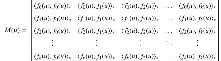
Definition 1.5.1 (Moment Matrix [18]) Given a linear formλ∈ _R[x]∗,x = (x1· · ·xn)which

maps a polynomial to a real number. A symmetric infinite matrix

M(λ)= (λ(xαxβ))α,β∈Nn (1.27)

is called amoment matrixofλwhereN={0,1,2,· · · }. We use graded lexicographic order for αandβthroughout this thesis.

Example 1.5.1 Consider λ = R[x,y]∗ such that λ = 1₂λ1,2 + 1₂λ2,1 (λ1,2 is the evaluation at

x=1,y=2andλ2,1 is the evaluation at x=2,y= 1). Let v= [1,x,y,x2,xy,y2, . . .]T

M(λ)=

       

1 3₂ 3₂ · · ·

3 2

5

2 2 · · · 3

2 2

5 2 · · ·

... ... ... ...        

= λ(v·vT). (1.28)

Theorem 1.5.1 [18] Given a moment matrix M(λ) corresponding to λ, We have λ(f2) =

vec(f) · M(λ) · vec(f)T

. In addition, M(λ) 0 if and only if λ is positive (Qλ is positive

semidefinite).

Theorem 1.5.2 Suppose λ ≥ 0. Then a polynomial p belongs to kerQλ if and only if its

coefficient vector belongs tokerM(λ). That is, we havekerQλ =kerM(λ).

Proof Givenλ≥0, we haveM(λ)0. SoQλ(f)= λ(f2)= 0 impliesvec(f)·M(λ)·vecT(f)=

0. SinceM(λ) 0,M(λ) has aCholesky factorization M(λ)= BBT_{. So}_vec₍_f₎_B₍_vec₍_f₎_B₎T =₀

which meansvec(f)B= 0 andM(λ)·vecT(f)=0.

Theorem 1.5.3 Supposeλ≥ 0. ThenkerQλ is an ideal, which is also real radical.

Proof Suppose f ∈kerQλ andgis an arbitrary polynomial, we need to show that f g∈kerQλ

as well. Nowλ(f2₎ = _{0 implies}_vec₍_f₎_· _M₍λ₎_·_vecT₍_f₎ = _{0 and}λ _≥ _{0 implies} _M₍λ₎ _{0. So}

we have M(λ)·vecT(f)= 0. From the structure of the moment matrix, it meansλ(xαf)= 0 for any monomialxα ∈_R[x]. Soλ(f2_g2₎= λ₍_{f g}2_· _f₎= λ₍₍_m

1+· · ·+mn)f)=0 wherem1,· · · ,mn

are monomials of f g2. So f g∈kerQλ.

(27)

1.5. Moment problem 15

1.5.2 Moment Problem

Theorem 1.5.4 (Riesz-Haviland’s Theorem [14]) For a linear formλ∈_R[x]∗

and closed set K inRn, the following two conditions are equivalent:

• λ(f)≥0for all f ∈_R[x]such that f ≥ 0on K

• There is a (positive) Borel measureµon K such thatλ(f)= R_K f dµfor all f ∈_R[X].

However, a nonnegative polynomial over Rn need not to be a sum of squares of polynomials

except in the univariate case (Hilbert 17th problem). For example the Motzkin polynomial

given by T.Motzkin [21]. It is the polynomial F(x,y) = x4y2 + x2y4+1− 3x2y2. (The non-negativity ofF(x,y) comes from the arithmetic-geometric mean inequality. Assume F(x,y) =

P

j f

2

j is a sum of squares of real polynomials. Then

P

j f

2

j(x,0) = M(x,0) = 1, which

means fj(x,0) are constants. Similarly fj(0,y) are constants. Hence each fj is of the form

fj =aj+bjxy+cjx2y+djxy2. By equating the coefficients ofx2y2, we have

P

jb

2

j = −3 which

is impossible.) So a natural question to ask is when does positivity of λon sums of squares indicate an integral representation with Borel measure?

Curto and Fialkow show the equivalence in the case that when M(λ) has finite rank, or dim(R[x]/kerQλ)=rank(M(λ)) is finite.

Theorem 1.5.5 (Curto and Fialkow [9]) Assume thatλ ≥ 0andrank(Mλ) = r < +∞. Then λ = Pr

i=1αiλvi for some distinct v1, . . . ,vr ∈ R

n _{and some real numbers} α

i > 0. λvi are

evaluations such thatλvi(f)= f(vi). Moreover,{v1, . . . ,vr}= VR(kerM(λ)).

1.5.3 Truncated Moment matrix and flat extension theorem

SupposeR[x]2d = {f ∈R[x]|deg(f)≤2d}, we can define the truncated linear formλd ∈R[X]∗2d

such that λd = λ|R[X]2d, the associated quadratic form Qλd and the truncated moment matrix

M(λd). Similarly, we define the truncated moment matrix.

Definition 1.5.2 (Truncated Moment Matrix [18]) Given a linear form λd ∈ (R[x]2d)∗, the

truncated moment matrix ofλdis defined to be

(28)

whereNnd ={γ∈N n

:|γ|= Σnj=1γj ≤d}.

Similarly, we have the following theorems for truncated linear forms and truncated moment

matrices.

Theorem 1.5.6 [18] Given a truncated moment matrix M(λd)corresponding toλd ∈ R[x]∗₂d,

M(λd)0(positive semidefinite) if and only ifλd ∈R[x]∗2dis positive.

Theorem 1.5.7 [18] A polynomial p ∈ _R[x]d belongs to kerQλd if and only if its coefficient

vector belongs tokerM(λd)∈R[x]d.

Example 1.5.2 Supposeλ1∈R[x,y]∗2andλ1(xayb)= ua,b. Then

M(λ1)=



   

u00 u10 u01

u10 u20 u11

u01 u11 u02



   

(1.30)

Without loss, we assume u00= 1.

The kernel of a positive semidefinite truncated moment matrix has the following “real

radical-like” property:

Lemma 1.5.8 [18] Assume M(λd) 0and let p,qj ∈ R[x], f := p2m+

P

jq2j with m ∈ N,

m≥1. Then, f ∈kerM(λd)⇒ p∈kerM(λd).

It also has the following ‘ideal-like” property:

Lemma 1.5.9 (Moment structure theorem, [18]) Letλd ∈R[x]∗2dand f,g∈R[x], f ∈kerM(λd).

(i)Assume M(λd) 0. ThenkerM(λd−1)⊆ kerM(λd)and f g∈kerM(λd)ifdeg(f g)≤d−1.

(ii) AssumerankM(λd) = rankM(λd−1). ThenkerM(λd−1) ⊆ kerM(λd)and f g ∈kerM(λd)if

deg(f g)≤d.

The ideal-like property is denoted as the RG condition in the works of Curto and Fialkow [9].

Definition 1.5.3 (ideal-like condition (RG condition))

(29)

1.6. Outline of the contents of the thesis 17

Theorem 1.5.10 (Flat extension theorem, [9]) Assume M(λd) ≥ 0. The following statements

are equivalent:

(i) There exists an extension of M(λd)onto M(λd+1)such that M(λd+1) 0andrankM(λd) =

rankM(λd+1)

(ii)kerM(λd)satisfies condition RG.

Lemma 1.5.11 [18] Assume M(λ) 0 and rankM(λd) = rankM(λd−1) = r. Then J =

hkerM(λd)iis real radical and zero-dimensional. One can extendλdtoλ¯ such thatλ¯ ∈R[x]∗.

Thenλis of the formλ = Pr

i=1αiλvi, whereαi > 0 and{v1, . . . ,vr} = VR(kerM(λd)). λvi are

evaluations such thatλvi(f)= f(vi). λ=λd when restricted toR[x]2d.

1.5.4 Generic linear forms

Assume an idealI = hh1, . . . ,hmiR. Ford∈N, define the set

Hd(I)={hixα |i= 1, . . . ,m,|α| ≤2d−deg(hi)} (1.31)

Define the set

Kd(I)= {λd ∈R[x]∗2d |λd(1)=1,M(λd) 0 andλd(f)= 0∀f ∈ Hd(I)} (1.32)

Theorem 1.5.12 [18] SupposeNd(I)=hkerM(λd)iandλdis a generic linear form (maximum

rank) in Kd(I). Then Nd(I) is independent of the particular choice of the generic element λd ∈ Kd(I).

Theorem 1.5.13 [18] We have:Nd(I)⊆ Nd+1(I)⊆ · · · ⊆

R √

I, with equalityhNd(I)iR=

R √

I for d large enough.

1.6 Outline of the contents of the thesis

(30)

1.6.1 Contents of Chapter 2

Geometric involutive bases for polynomial systems of equations have their origin in the

pro-longation and projection methods of the geometers Cartan and Kuranishi for systems of PDE.

They are useful for numerical ideal membership testing and the solution of polynomial

sys-tems. In this chapter we further develop our symbolic-numeric methods for such bases. We

give methods to explicitly extract and decrease the degree of intermediate systems and the

output basis. Algorithms for the numerical computation of involutivity criteria for positive

dimensional ideals are also discussed.

We were also motivated by some remarkable recent work by Lasserre and collaborators

who employed our prolongation projection involutive criteria as a part of their semi-definite

based programming (SDP) method for identifying the real radical of zero dimensional

polyno-mial ideals. Consequently in this chapter we begin an exploration of the interaction between

geometric involutive bases and these methods particularly in the positive dimensional case.

Motivated by the extension of these methods to the positive dimensional case we explore the

interplay between geometric involutive bases and the new SDP methods.

1.6.2 Contents of Chapter 3

For a real polynomial system with finitely many complex roots, the real radical ideal, RRI, is

generated by a lower degree system that has only real roots and the roots are free of

multiplic-ities. The RRI is a central object in computational real algebraic geometry. The computation

of such RRI is of practical interest since multiplicities of roots yield singular Jacobians and

cause problems for numerical solvers. Moreover the number of real roots can be far less than

the number of complex roots and Lasserre and co-authors have shown that the RRI of a

0-dimensional real polynomial system with finitely many real solutions can be determined by

a combination of techniques from a semidefinite programming (SDP) feasibility problem and

geometric involution. A conjectured extension of such methods to positive dimensional

poly-nomial systems has been given recently by Ma, Wang and Zhi.

In this section we show that regularity in the form of the Slater constraint qualification

(31)

1.6. Outline of the contents of the thesis 19

reduction and obtain a smaller regularized problem for which strict feasibility holds. We use

this framework for analyzing RRIs of 0 and positive dimensional real polynomial systems. The

SDP methods are implemented in MATLAB and our geometric involutive form is implemented

in Maple. We consider two approaches to find a feasible moment matrix. We compare the

SeDuMi interior point approach within the YALMIP package for MATLAB with the

Douglas-Rachford (DR) projection-reflection method.

Illustrative examples show the advantages of the DR approach for some problems over

stan-dard interior point methods. We also see the advantage of facial reduction both in regularizing

the problem and also in reducing the dimension of the moment matrices.

1.6.3 Contents of Chapter 4

Recent breakthroughs have been made in the use of semidefinite programming and its

appli-cation to real polynomial solving. For example, the real radical of a zero dimensional ideal,

can be determined by such approaches as shown by Lasserre and collaborators. Some progress

has been made on the determination of the real radical in positive dimension by Ma, Wang and

Zhi. Such work involves the determination of maximal rank semidefinite moment matrices.

Existing methods are computationally expensive and have poorer accuracy on larger examples.

In previous work we showed that regularity in the form of the Slater constraint

qualifi-cation (strict feasibility) fails for the moment matrix in the SDP feasibility problem. We used

facial reduction to obtain a smaller regularized problem for which strict feasibility holds.

How-ever we did not give a theoretical guarantee that our methods, based on facial reduction and

Douglas-Rachford iteration ensured the satisfaction of the maximum rank condition to possibly

approximate the real radical characterizing all real roots.

This chapter is motivated by the problems above. We discuss how to compute the moment

matrix and its kernel using facial reduction techniques where the maximum rank property can

be guaranteed by solving the dual problem. The facial reduction algorithms on the primal

form is presented. We give examples that exhibit for the first time additional facial reductions

beyond the first which can be computed in practice.

(32)

we give and prove an algorithm for computing the real radical up to any given finite degree.

We also prove results regarding the well-posedness of our approach.

1.6.4 Conclusions are given in Chapter 5

1.6.5 Appendices

Bibliography

[1] Teijo Arponen, Samuli Piipponen, and Jukka Tuomela. Kinematic analysis of bricards

mechanism. Nonlinear Dynamics, 56(1-2):85–99, 2009. 1

[2] Daniel J Bates, Jonathan D Hauenstein, Andrew J Sommese, and Charles W Wampler.

Numerically solving polynomial systems with Bertini, volume 25. SIAM, 2013. 4, 25 [3] Eberhard Becker and Rolf Neuhaus. Computation of real radicals of polynomial ideals.

InComputational algebraic geometry, pages 1–20. Springer, 1993. 7

[4] J.M. Borwein and H. Wolkowicz. Facial reduction for a cone-convex programming

prob-lem. J. Austral. Math. Soc. Ser. A, 30(3):369–380, 1980/81. 12, 54, 94, 98, 106

[5] J.M. Borwein and H. Wolkowicz. Regularizing the abstract convex program. J. Math. Anal. Appl., 83(2):495–530, 1981. 12, 54, 94, 98, 106

[6] D. Brake, J. Hauenstein, and A. Liddell. Numerically validating the completeness of the

real solution set of a system of polynomial equations.Procedings of the 41th International Symposium on Symbolic and Algebraic Computation, 2016. 1, 115, 118, 121, 130 [7] Y-L. Cheung, S. Schurr, and H. Wolkowicz. Preprocessing and regularization for

degen-erate semidefinite programs. In D.H. Bailey, H.H. Bauschke, P. Borwein, F. Garvan,

(33)

Bibliography 21

[8] David Cox, John Little, and Donal O’shea. Ideals, varieties, and algorithms, volume 3. Springer, 1992. 2, 7, 113

[9] RE Curto and LA Fialkow. Solution of the truncated complex moment problem for flat

data-introduction.Memoirs of the American Mathematical Society, 119(568):1, 1996. 13, 15, 16, 17, 25, 108, 109, 110

[10] D. Drusvyatskiy, N. Krislock, Y-L. Cheung Voronin, and H. Wolkowicz. Noisy sensor

network localization: robust facial reduction and the Pareto frontier. Technical report,

University of Waterloo, Waterloo, Ontario, 2014. arXiv:1410.6852, 20 pages. 12, 54, 94

[11] D. Drusvyatskiy, G. Pataki, and H. Wolkowicz. Coordinate shadows of

semi-definite and euclidean distance matrices. Math. Programming, 25(2):1160–1178, 2015. ArXiv:1405.2037.v1. 12, 98

[12] V.P. Gerdt and Y.A. Blinkov. Involutive bases of polynomial ideals. Mathematics and Computers in Simulation, 45(5):519–541, 1998. 7, 24, 29, 59, 112

[13] Jonathan D Hauenstein. Numerically computing real points on algebraic sets. Acta ap-plicandae mathematicae, 125(1):105–119, 2013. 5, 26, 83, 85, 121

[14] E. K. Haviland. On the momentum problem for distribution functions in more than one

dimension. ii. American Journal of Mathematics, 58(1):164–168, 1936. 15

[15] N. Krislock and H. Wolkowicz. Explicit sensor network localization using semidefinite

representations and facial reductions. SIAM Journal on Optimization, 20(5):2679–2708, 2010. 12, 54, 94

[16] J.B. Lasserre, M. Laurent, and P. Rostalski. A prolongation–projection algorithm for

com-puting the finite real variety of an ideal. Theoretical Computer Science, 410(27):2685– 2700, 2009. 1, 8, 25, 47, 53, 54, 55, 64, 84, 93, 94, 120

[17] Jean Bernard Lasserre, Monique Laurent, and Philipp Rostalski. Semidefinite

(34)

[18] M. Laurent and P. Rostalski. The approach of moments for polynomial equations. In

Miguel F. Anjos and Jean B. Lasserre, editors, Handbook on semidefinite, conic and polynomial optimization, International Series in Operations Research & Management Science, 166, pages 25–60. Springer, New York, 2012. 10, 13, 14, 15, 16, 17, 36, 38,

40, 46, 47, 58, 95, 96, 128, 129

[19] Y. Ma. Polynomial Optimization via Low-rank Matrix Completion and Semidefinite Programming. PhD thesis, Academy of Mathematics and Systems Science, Chinese Academy of Science, 2012. 8, 53, 55, 62, 77, 84, 93, 120, 121

[20] Y. Ma, C. Wang, and L. Zhi. A certificate for semidefinite relaxations in computing

positive dimensional real varieties. Journal of Symbolic Computation, 72:1 – 20, 2016. vii, x, 1, 8, 53, 55, 62, 77, 78, 79, 80, 81, 82, 84, 93, 120, 121, 128, 129

[21] Theodore Samuel Motzkin. The arithmetic-geometric inequality. In: Proc. Symposium on Inequalities, edited by O. Shisha, pages 205–224, 1967. 15

[22] James D Murray. Mathematical Biology. II Spatial Models and Biomedical Applications

{Interdisciplinary Applied Mathematics V. 18}. Springer-Verlag New York Incorporated, 2001. 1

[23] Rolf Neuhaus. Computation of real radicals of polynomial idealsii. Journal of Pure and Applied Algebra, 124(1):261–280, 1998. 8

[24] G. Pataki. Strong duality in conic linear programming: facial reduction and extended

duals. In David Bailey, Heinz H. Bauschke, Frank Garvan, Michel Thera, Jon D.

Vander-werff, and Henry Wolkowicz, editors, Computational and analytical mathematics, vol-ume 50 ofSpringer Proc. Math. Stat., pages 613–634. Springer, New York, 2013. 12, 13

[25] G. Reid, F. Wang, H. Wolkowicz, and W. Wu. Semidefinite Programming and facial

(35)

Bibliography 23

[26] A.J. Sommese and C.W. Wampler. The Numerical solution of systems of polynomials arising in engineering and science, volume 99. World Scientific, 2005. 1, 4, 25, 53, 93 [27] F. Sottile. Real solutions to equations from geometry, volume 57 of University Lecture

Series. American Mathematical Society, Providence, RI, 2011. 8, 53, 54, 55, 56, 84, 93, 94, 120

[28] Silke J Spang. On the computation of the real radical. PhD thesis, Thesis, Technische Universit¨at Kaiserslautern, 2007. 7

[29] Levent Tunc¸el. Polyhedral and semidefinite programming methods in combinatorial op-timization, volume 27 of Fields Institute Monographs. American Mathematical Society, Providence, RI, 2010. 13

[30] Jan Verschelde. Algorithm 795: Phcpack: A general-purpose solver for polynomial

sys-tems by homotopy continuation. ACM Transactions on Mathematical Software (TOMS), 25(2):251–276, 1999. 4

[31] H. Wolkowicz, R. Saigal, and L. Vandenberghe, editors. Handbook of semidefinite pro-gramming. International Series in Operations Research & Management Science, 27. Kluwer Academic Publishers, Boston, MA, 2000. Theory, algorithms, and applications.

10, 11, 12, 68

[32] W. Wu and G.J. Reid. Finding points on real solution components and applications to

(36)

Geometric involutive bases for positive

dimensional polynomial ideals and SDP

methods

2.1 Introduction

This paper is part of a stream devoted to developing symbolic-numeric prolongation projection

algorithms for general systems of partial and differential algebraic equations. Such algorithms prolong (differentiate) such systems and project the prolonged systems to determine obstruc-tions or missing constraints to their integrability. See Kuranishi [18] for proof of termination

of such methods using Cartan’s geometric involutivity criteria. A by-product of these

meth-ods has been their implementation for linear homogeneous partial differential equations with constant coefficients, and consequently for polynomial algebraic systems. See [13] for appli-cations and symbolic algorithms for polynomial systems. The symbolic-numeric version of a

geometric involutive form was first described and implemented in Wittkopf and Reid [41]. It

was applied to approximate symmetries of differential equations in [6] and to polynomial solv-ing in [32, 31, 35]. See [43] where it is applied to the deflation of multiplicities in multivariate

polynomial solving.

The current paper is focused on further development of our geometric involutive basis

(37)

2.1. Introduction 25

gorithm particularly in the positive dimensional case, and also in relation to real solving. It

is especially motivated by remarkable recent developments concerning real solution of such

systems by Lasserre, Laurent and Rostalski [19] and their use of aspects of our prolongation

projection algorithm in the paper “A prolongation-projection algorithm for computing the fi-nite real variety of an ideal”. They developed a new approach for computing the real radical of zero dimensional polynomial systems using semi-definite programming (SDP) techniques. See

[10] for early fundamental work on such problems. Zero dimensional systems are those having

finitely many real solutions, and the real radical is the set of polynomials which vanish on these

solutions. In contrast to the input systems the output radical systems from their approach are

multiplicity free and so are better conditioned for numerical solution techniques. The output

radical systems only have real roots and no complex roots. This leads to possibility of lower

complexity methods, since current methods for finding real solutions, mostly explicitly, or

im-plicitly pass through complex root formulations. Given the widespread popularity of linear

programming (and by implication) SDP methods, the surprising links between this area also

open interesting research possibilities. See [4] for a recent book on the connections between

semi-definite optimization and convex algebraic geometry.

We briefly list some background references. There have been considerable recent advances

in numerical complex geometry. See especially the books [38, 2] and the references therein.

In approaches based on homotopy continuation, positive dimensional components characterize

the variety over C by certain witness points cut out by intersections of the components with

random linear spaces. For a modern text with many references on computational real algebraic

geometry see [1]. Real algebraic geometry is a vast subject with many applications. Sturm’s

ancient method on counting real roots of a polynomial in an interval is central to Tarski’s

real quantifier elimination [40] and was further developed by Seidenberg [36]. One of the

most important algorithms of real algebraic geometry is cylindrical algebraic decomposition.

CAD was introduced by Collins [9] and improved by Hong [17] who made Tarski’s quantifier

elimination algorithmic. This algorithm decomposes_Rn _{into cells on which each polynomial}

of a given system has constant sign. The projections of two cells in Rn to Rk with k < n

either don’t intersect or are equal. The computational cost of this algorithm, which is doubly

(38)

using triangular decompositions. For approaches based on obtaining witness points for the real

positive dimensional case see [34, 15, 16, 42]. Homotopy methods are used in [21] and [3] for

real algebraic geometry. Recently such moment matrix completion techniques are explored by

Zhi et al in [22] for finding at least one real root of a given semi-algebraic system. Furthermore,

based on critical point technique and moment matrix completion, they studied the computation

of verified real solutions on positive dimensional system in [44].

As part of our initial exploration of this area, in this paper, we make some improvements

in our geometric involutive bases, by enabling the explicit extraction of projected systems and

hence reducing the size of matrices that can appear in intermediate computations. Similarly

motivated by the extension of these methods to the positive dimensional case we explore the

interplay between geometric involutive bases and the new SDP methods. The symbol space

of a polynomial system or kernel of the matrix of its highest coefficients is the geometric generalization of the highest coefficient of a polynomial. Certain projections within the symbol space encode a geometric test - an analogue of the S-polynomials in Gr¨obner basis approaches

- for new members of the polynomial ideal. We provide details and example of this in the

numerical case. An attempt in this paper is made to minimize use of terminology from the jet

geometry of partial differential equations, in order to make this accessible to a wider audience.

2.2 Brief background on ideals and varieties

In this section we briefly sketch some basic objects from real and complex algebraic geometry

and introduce some notation for our paper.

2.2.1 Some basic objects in complex algebraic geometry

Consider the setC[x1,x2, ...,xn] of multivariate polynomials with complex coefficients in the

complex variables x = (x1,x2, ...,xn) ∈ Cn. Then C[x1,x2, ...,xn] is a ring. Given P = {p1(x),p2(x), ...,pm(x)} ⊆C[x1,x2, ...,xn]=C[x] its solution set or variety is:

VC(p1,p2, ...,pm)=

(39)

2.2. Brief background on ideals and varieties 27

For brevity we sometimes write VC(P) = {x ∈ C

n

: P(x) = 0}. Upper case letters P, Q,

R, etc will denote sets of polynomials and lower case letters p, q etc will denote individual polynomials.

The ideal over_Cgenerated byP= {p1, ...,pk}is:

hPi_C= hp1, ...,pki_C= {f1p1+...+ fkpk : fj ∈C[x],1≤ j≤ k} (2.2)

and its associated radical ideal overCis

C

p

hPi_C = {f ∈_C[x] : f(x)=0 for all x∈VC(P)}

= {f ∈_C[x] : fm∈ hPi_C for some m∈_N} (2.3) whereNis the set of non-negative integers.

Example 2.2.1 To make this paper accessible to a wide audience we illustrate first some of the main ideas on the simple and well-known case of systems of univariate polynomials. Given a system of k univariate polynomials P = {p1, ...,pk} with coefficients from some computable

field (e.g.Q), a Gr¨obner basis (orgcd) computation returns a single polynomial q(x):

hqi_C =hp1, ...,pki_C (2.4)

The factorization of q(x)overChas form:

q(x)= a(x−a1)n1...(x−a`)n` (2.5)

where the roots aj ∈Cof q(x)are distinct. Though the ajcan’t be found in general by finitely

many rational operations the so-called square-free factorization can be found by such opera-tions yielding:

˜

q(x)= q(x)

gcd(q(x),q0₍_x₎₎ = a(x−a1)...(x−a`) (2.6)

For this example the ideal, variety and radical ideal overCare:

hPi_C = {g(x)·(x−a1)n1...(x−a`)n` :g(x)∈C[x]}

V_C(P) = {a1,a2, ...,a`} (2.7)

C

p

hPi_C = {g(x)·(x−a1)...(x−a`) :g(x)∈C[x]}

(40)

2.2.2 Some basic objects in real algebraic geometry

Suppose that x = (x1,x2, ...,xn) ∈ Rn and consider a system of k multivariate polynomials

P = {p1(x),p2(x), ...,pk(x)} ⊆ R[x1,x2, ...,xn] with real coefficients. Its solution set or variety

is

VR(p1, ...,pk)={x∈Rn: pj(x)= 0, 1≤ j≤ k} (2.8)

The ideal generated byP={p1, ...,pk} ⊆ Ris:

hPi_R= hp1, ...,pki_R= {f1p1+...+ fkpk : fj ∈R[x],1≤ j≤ k} (2.9)

and its associated radical ideal over_Ris defined as

R

p

hPi_R = {f ∈_R[x] : f2m+ Σs_j₌₁q2_j ∈ hPi_R for someqj ∈R[x],m∈N\{0}} (2.10)

A fundmental result [5] (originally proved in [33]) is:

Theorem 2.2.1 [Real Nullstellensatz] For any ideal I⊆ _R[x]we have √R

I = I(VR(I)).

Consequently

R

p

hPi_R = {f(x)∈_R[x] : f(x)= 0 for all x∈VR(P)} (2.11)

Remark An idealI ⊆_R[x] is real radical if and only if for all p1,· · · ,pk ∈R[x]:

p2₁+· · ·+ p2k ∈I =⇒ p1,· · · ,pk ∈I. (2.12)

For these and many other results see [1] and the references cited therein.

Example 2.2.2 Consider the simplest case of a system of k univariate polynomials in some computable subfield of R (e.g. Q). Then as in the complex case a Gr¨obner basis of such a

system yields a single polynomial q(x) having the same roots. Discarding the factors with complex roots with nonzero imaginary parts yields a polynomial of form:

˜

q(x)=b(x−b1)m1...(x−bj)mj (2.13)

where b1, b2, ... , bjare the real roots and m1, ... , mj their corresponding multiplicities. Then hPi_R = {f(x)·(x−b1)m1...(x−bj)

mj _: _f₍_x₎_∈

R[x]}

VR(P) = {b1,b2, ...,bj} (2.14) R

p