Solar and Wind Power System Frequency Control by
Flow Control of HVDC Interconnection Line
Raghu.Kochcharla Assistant Professor
Sayyad Rajiya Begum Assistant Professor
Department of EEE
Medha Institute of Science and Technology for Women, Khammam, Telangana India.
Abstract: In recent years, environmental problems are being serious and renewable energy
has attracted attention as their solutions. However, the electricity generation using the renewable energy has a demerit that the output becomes unstable because of intermittent characteristics such as variations of wind speed or solar radiation intensity. Therefore, it can cause frequency fluctuations or voltage fluctuations in the power system. Various methods have been investigated and reported so far to control the frequency and voltage fluctuations. This paper presents a new control method to suppress the frequency fluctuations occurring due to a large amount of photovoltaic (PV) power generation and wind power generation, which is based on power flow control of High voltage direct current (HVDC) interconnection line and using a dead band in its frequency control system.
Index Terms: High voltage direct current (HVDC), Power system frequency control, Dead band, PV power generation and Wind power generation.
I. INTRODUCTION
Various studies for renewable energy systems, such as wind power generation, PV power generation, geothermal power generation, etc., have been carried out so far. Wind power generation has some merits that the generation cost is relatively low and the energy conversion efficiency is higher compared to other electricity generation using the renewable energy. Also PV power generation has some merits that the power generation efficiency is almost constant irrespective of the scale of the system to be installed and that no noise are generated during power generation. However, the electricity generation using such renewable energy systems may cause frequency and voltage fluctuations in the power system
Fig. 1. Model system.
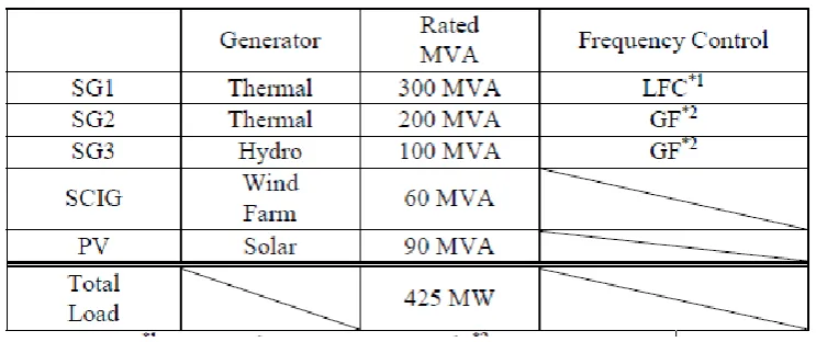
Table I: Conditions Of Each Generator
*1LFC: Load Frequency Control, *2GF: Governor Free
2.
MODEL SYSTEM
A. Power System Model
The power system model used in this study and its parameters are shown in Fig. 1. It is a modified version of the IEEE standard model with 9 buses which is composed of 3 synchronous generators (SG1, SG2, and SG3). SG1 and SG2 are thermal power plants (SG1: 300MVA, SG2: 200MVA), and SG3 is a hydraulic power plant
(100MVA). Moreover, a wind farm (WF) composed of 20 squirrel cage induction generators (SCIGs), a PV station, HVDC interconnection line, and three loads (Loads A, B, and C) are connected to the main system . Their conditions are shown in Table Ι. The HVDC transmission line is lies between the main modified 9-bus power system and another large power system (infinite bus) and the direction of the power flow is from main power system to the infinite bus.
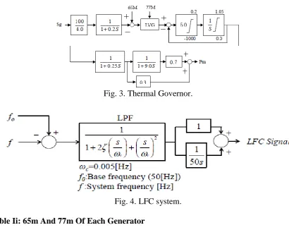
Fig. 3. Thermal Governor.
Fig. 4. LFC system.
Table Ii: 65m And 77m Of Each Generator
B. Governor Model
Governor is a device for controlling the rotational speed of the synchronous generator and turbine. When the balance between the turbine output and generator output does not hold, the rotational speed changes. In order to return the rotation speed to the synchronous speed, the turbine output is controlled by the governor system. There are various frequency components in the power supplied to the power system from the wind generators and PV stations, resulting in frequency fluctuations of the power system. Conventional thermal and hydro governors control their turbine output to suppress the frequency fluctuations, in which short period components of from a
few tens of seconds to a few minutes are controlled by the governor free (GF) operation and relatively long period components of from a few minutes to several tens of minutes are controlled by the load frequency control (LFC). These control blocks used in this paper are shown in Figs. 2 and 3. A hydraulic generator speed governor model used in the simulation analyses is shown in Fig. 2, where
Sg: Rotation speed deviation
65M: Load setting (Output reference value) 77M: Load limit (65M+rated output×PLM[%])
Input values of 65M and 77M are shown in Table II. The governor operating margin is set to ± 5% of the governor rated output. Thermal generator speed governor model and the LFC system model used in the simulation analyses are shown in Figs. 3 and 4. Load frequency control (LFC) supplies output command signal to the power plants according to the frequency deviation. The LFC signal is input to 65M, and then, the output of each power plant is changed. The frequency deviation is input to the Low Pass Filter (LPF) to remove components of short period as shown in Fig. 4, and then LFC signal is generated through PI controller. This is because the LFC is used to control frequency fluctuations with a long period of time. The angular frequency ωc (=2πf) of LPF is set to 0.005 [Hz]. The governor models used in this paper are based on the standard models of the Institute of Electrical Engineers of Japan.
C. Wind Turbine Model
Wind turbine model used in this paper is shown in eqs. (1) - (5).
Where, Pwtb: wind turbine output [W], λ: tip speed ratio, R: wind turbine radius [m],
ωWtb: wind turbine angular speed [rad/s], β: pitch angle [deg], Vw: wind speed [m/s], ρ: air density [kg/m3], Cp: power coefficient,
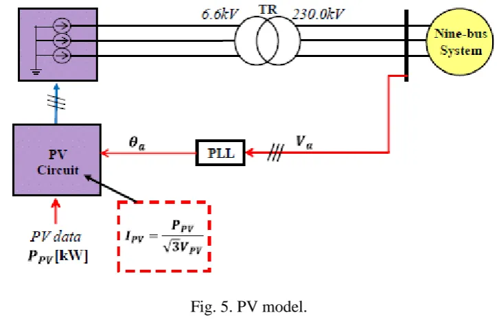
Ct: torque coefficient, τm: wind turbine torque [Nm] D. PV System PV model used in this study is shown in Fig. 5. In this study, the PV model is expressed by a simple model using current sources, in which kilowatts data, PPV [kW], is used.Therefore, PV current (IPV) is calculated from PPV [kW] and VPV [kV], and the obtained current (IPV) is entered to the current sources. PV voltage (VPV) is fixed at 6.6 kV.
Fig. 5. PV model.
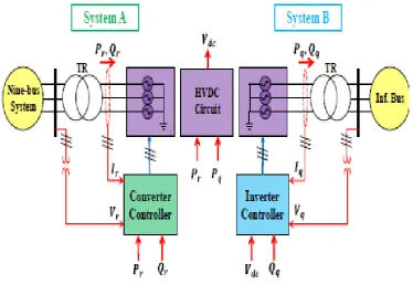
The HVDC system model used in this study is shown in Fig. 6. In this study, to shorten the calculation time of the simulation, the HVDC model is expressed by a simple model using controlled voltage sources instead of IGBT based inverter and rectifier. (1) Control model of system A side converter The control block of the converter that converts from threephase AC to DC voltage is designed as shown in Fig. 7. First, the phase angle is obtained by detecting the phase voltage Vr from the three-phase terminal voltage at the converter. Next, the d-axis and q-axis components (Ird, Irq) of the current are obtained from the phase angle and the three-phase current. Active power Pr and reactive power Qr of the converter are controlled independently by the d-axis and the q-axis components. For this purpose, the d-axis and q-axis components (Vrd *, Vrq *) of the voltage are obtained through the PI controller. An output reference value Pref is determined so as to suppress system frequency fluctuations
(described later). Finally, the d-axis and q-axis voltages are converted to three-phase AC voltages. The parameters of PI controllers (PI1, PI2) are shown in TABLE III. (2) Control model of system B side inverter .The control block of the inverter that converts the DC voltage to the three-phase AC is designed as shown in Fig. 8. As shown in Fig. 8, the phase angle is obtained by detecting the phase voltage Vq from the three-phase terminal voltage at the inverter. Next, the d-axis and q-axis components (Iqd,
Iqq) of the current are obtained from the phase angle and the three-phase current. DC voltage Vdc of the HVDC line and reactive power output Qq of the inverter are controlled by the d-axis and q-axis components. For this purpose, the daxis and q-axis components (Vqd *, Vqq *) of the voltage are obtained through the PI controller. Finally, the d-axis and qaxis voltages are converted to three-phase AC voltages. The parameters of PI controllers (PI3, PI4) is shown in TABLE III.
Fig. 7. Converter control system.
Fig. 8. Inverter control system.
Table III: Parameters of Pi Controller
F. DC-Link model
The DC-Link model is shown in Fig. 9, in which the DClink voltage is expressed by eq. (6).
Where, Vdc: DC Voltage, Cdc: Capacitance of smoothing capacitor in the DC link (50,000μF), Pr: Active power of the converter, Pq: Active power of the inverter, Vdcn: Rated voltage of the HVDC line (250kV).
G. Dead band type frequency control
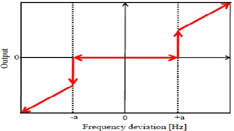
Fig. 10 shows a block diagram of the proposed frequency control with dead band for the HVDC line, where Pref denotes a reference for HVDC line power flow and it is determined according to the frequency deviation Δf [Hz] of the main system
(System A). In Fig. 10, ΔP=0 when Δf [Hz] is less than the threshold value “a” [Hz] in the dead band, and Δf *P gain is sent to the adder when Δf [Hz] is greater than the threshold value. Target value Pref of the HVDC line flow is calculated by adding ΔP to the steady state reference value, PDC0 (= 0.5 [p.u.] in this study). Therefore, HVDC line flow is composed of compensating component for the frequency fluctuations and the steady state reference. In Fig. 11, the output image of the dead band is shown. The threshold value “a” of the dead band is set to 0.06 [Hz] in this paper, and P Gain is set to
%KG = 14.9, which is the system constant of System A. The equation about the system constant %KG is shown in eq. (7). KG is the amount of total
generator output which needs to change the system frequency by 1 [Hz].
Fig. 10. Frequency control system with dead band by HVDC.
III. SIMULATIOM RESULTS
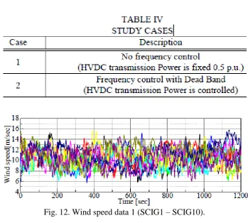
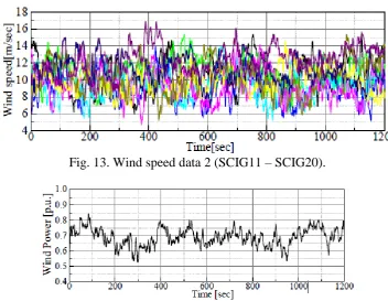
To confirm the effectiveness of the proposed method, simulation analyses have been performed for 2 cases, in which fixed power flow of HVDC line is referred “No frequency control” and the proposed frequency control with dead band by HVDC line is referred “with Dead band”. The 2 cases are shown in TABLE IV. The wind speed data used in the simulation analyses is shown in Fig. 12 and 13. This is real wind speed data measured in Hokkaido Island, Japan. The total output of 20 wind turbine generators is shown in Fig. 14. The PV data used in the simulation analyses is shown in Fig. 15. This is also real PV data measured in Hokkaido Island, Japan. The total output of 20 wind turbine generators and PV station is shown in Fig. 16. Simulation results of
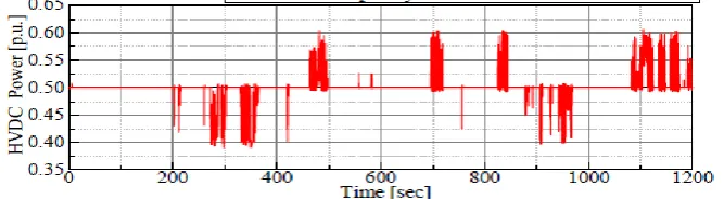
two cases are shown Fig. 17 and 18. Fig. 17 shows responses of the system frequency and it is seen the frequency variations exceed ±0.1Hz in the case of “No frequency control”, but the frequency variations are well controlled in the case of “with Dead Band”. Fig. 18 shows power flow of HVDC line, in which the power flow is fixed at 0.5 [p.u.] in the case of “No frequency control”. In the case of “with Dead band”, power flow of the HVDC line is controlled by the proposed frequency control system according to the frequency fluctuations. Table V shows the maximum deviation and standard deviation of the system frequency fluctuations, from which it is also seen that the proposed HVDC power flow control system can suppress the system frequency luctuations effectively.
TABLE IV STUDY CASES
Fig. 13. Wind speed data 2 (SCIG11 – SCIG20).
Fig. 14. Total output of wind power generators.
Fig. 15. Output of PV station.
Fig. 16. Total output of WF and PV.
Fig. 18. Comparison of HVDC transmission Power.
TABLE V: MAXIMUM DEVIATION AND STANDARD DEVIATION OF SYSTEM FREQUENCY
IV. CONCLUSION
In order to suppress the frequency fluctuations in the power system with large amount of PV and WF installed, a new method of frequency control with dead band by HVDC interconnection line is proposed in this paper, and its validity is examined through simulation analyses. As a result, it is shown that the proposed control method can suppress the frequency fluctuations effectively. As in this study control of amount of energy transmitted through the HVDC line during a specified period (simultaneous/commensurate regulation) is not taken into account, the authors are planning to extend the control system which can also control the transmitted energy through the HVDC line.
V. REFERENCES
1. P. M. Anderson, A. A. Found: Power System Control and Stability, IEEE Press, 1994.
2. M. Rosyadi, A. Umemura, R. Takahashi, J. Tamura, N. Uchiyama, K. Ide, “Simplified Model of Variable Speed Wind Turbine Generator for Dynamic Simulation Analysis,” IEEJ Trans. of Power System Power and
Energy, Vol.135, No.9,
pp.538-549,2015.
and Energy, Vol.134, No.5,
pp.393-398,2014.
4. O. Wasynczuk, D. T. Man and J. P. Sullivan, “Dynamic Behavior of a Class of Wind Turbine Generators During Randon Wind
5. Fluctuations,” IEEE Trans. On Power
Apparatus and System, vol. PAS-100,
no. 6, pp. 2837-2845, June 1981. 6. T. Sato, A. Umemura, R. Takahashi, J.
Tamura, “Frequency Control of Power System with Large Scale Wind Farm Installed by Using HVDC Transmission System,” IEEE PES
PowerTech 2017, No.108(USB
6pages) Manchester, United Kingdom, June 2017.
7. T. Ono, J. Arai, “Frequency Control with Dead Band Characteristic of Battery Energy Storage System for Power System Including Large Amount of Wind Power Generation”
IEEJ Trans. PE, Vol.132, No.
8,pp.709-717,2012.
8. Y. Yoshida, K. Koiwa, A. Umemura, R. Takahashi, and J. Tamura: “Power System Frequency Control with Dead Band by Using Kinetic Energy of Variable Speed Wind Power Generator”, Proc. of the 2015 IEEE Energy Conversion Congress and
Exposition (ECCE2015), NO.160,
pp.470-476, Montreal, Canada (2015/9).
Raghu.Kochcharla working as an Assistant Professor in EEE Department at Medha Institute of Science and Technology for Women, having 5 years of teaching experience. His area of specialization is in the fields of Power Systems and Electrical Machines using Power Electronic Devices. He guided so
many number of graduating and Post graduating engineering projects. He had published the some papers in different fields of Electrical engineering.