Comparison of turbulence models and CFD solution options for a plain pipe

(1)

*

Comparison of turbulence models and CFD solution options for

a plain pipe

Eyub Canli1,*_,_Ali_Ates1_{, and}_Sefik_Bilir1

1_{Selcuk University, Mechanical Engineering Department, P.K. 42003 Selcuklu Konya, Turkey}

Abstract. Present paper is partly a declaration of state of a currently ongoing PhD work about turbulent flow in a thick walled pipe in order to analyze conjugate heat transfer. An ongoing effort on CFD investigation of this problem using cylindrical coordinates and dimensionless governing equations is identified alongside a literature review. The mentioned PhD work will be conducted using an in-house developed code. However it needs preliminary evaluation by means of commercial codes available in the field. Accordingly ANSYS CFD was utilized in order to evaluate mesh structure needs and asses the turbulence models and solution options in terms of computational power versus difference signification. Present work contains a literature survey, an arrangement of governing equations of the PhD work, CFD essentials of the preliminary analysis and findings about the mesh structure and solution options. Mesh element number was changed between 5,000 and 320,000. k-ϵ, k-ω, Spalart-Allmaras and Viscous-Laminar models were compared. Reynolds number was changed between 1,000 and 50,000. As it may be expected due to the literature, k-ϵ yields more favorable results near the pipe axis and k-ω yields more convenient results near the wall. However k-ϵ is found sufficient to give turbulent structures for a conjugate heat transfer problem in a thick walled plain pipe.

1 Introduction

Flow inside a thick walled pipe and related heat transfer is of interest. Numerical and computational means can be used for investing a wide range of mentioned interest and compact results can be reported in a way that the results can be converted and applied to a wide application variety and field. The compact results can be derived by scaling and using dimensionless governing equations.

A dedicated team in Turkey has been performing numerical studies on unsteady and steady conjugate heat transfer related to thick walled pipes under various conditions such as periodic boundary conditions, simultaneously developing flow, rarefaction effects and slippery flow, heat transfer in tangential direction and etc by using cylindrical coordinates and their own developed codes. As mentioned earlier, the results are dimensionless and can be expanded for certain magnitudes. Remarkable developments and major events are summarized below according to the publishing timeline.

After a detailed and informative PhD dissertation was published in 1988 [1] about heat transfer in laminar pipe flow in the thermal development region at low Peclet numbers including axial conduction, Bilir (1995) reported a numerical laminar heat transfer analysis including two dimensional axial conduction for the wall and for the fluid [2]. The pipe in the problem was constituted by two regions and second region causes a

step change in outside surface temperature. This causes heat transfer through the wall and the fluid. Peclet number, thickness ratio and wall-to-fluid conductivity ratio were taken as the investigated parameters while Peclet number was found as the most effective parameter among them. It should also worth that the numerical code of [1] is also given in it. Bilir then reported a solution for transient regime of the previously mentioned problem [3]. This time parameters were increased as wall-to-fluid thermal diffusivity ratio was added into the analysis. As a main conclusion of the work, author reported that the time passed in order to reach the steady state conditions does not change significantly with the parameters although the early and intermediate periods exhibit differences. It was also stressed that flow conditions determine the thermal inertia rather than the wall specifications.

(2)

reported [6]. Their main findings can be summarized as the preheating phenomenon due to the axial heat transfer towards the upstream; reverse heat flow (from fluid to wall) at the early transient stages in upstream; peak values at the interface of upstream and downstream due to the surpassing radial wall conduction; and axial heat conduction towards downstream region through the wall in steady state conditions making the heat flux values at fluid wall interface greater than the outer surface where heat flux boundary condition exists.

First time numerical solution of the flow of the team was in 2004 where laminar flow development was obtained for simultaneously developing flow [7]. The effect of the velocity profile other than the parabolic velocity profile is investigated and results are given comparatively in terms of the outer and inner wall temperatures, bulk temperatures, radial distributions of the fluid temperatures and Nusselt numbers [8]. It is said that velocity profile has no effect on interface and outer surface temperatures. Bulk temperature values on the other hand are higher for developing flow comparing to the developed flow. Slug flow for the thick walled pipe is also examined numerically by the team [9]. For this flow type, temperature profiles develop faster in the order of outer surface, interface and bulk flow. They validated their results by considering the Nusselt number for developed flow with constant temperature condition. Since thick walled pipes can be seen in applications involving micro-channels and mini-pipes frequently, the parameters were arranged by the authors and reported [10]. There are six parameters which are wall thickness ratio, fluid thermal conductivity ratio, wall-to-fluid thermal diffusivity ratio, the Peclet number, the Biot number and the Prandtl number. It is stated that the interfacial heat flux rises rapidly at initiation of the transient regime due to fast radial conduction in the wall at the entrance of the pipe. Then it reaches a constant value in a short axial distance. Again it is noticed that heat flux values decrease in the mean and uniformity of the curves are deformed as time elapses because of the increasing effect of convection in the fluid side and after a maximum they decrease in the flow direction. As an analogy to electrical current, conjugation increases with the diameter. Remaining parameters reduce it. The critic values of the parameters are also given and after these critic values towards a certain direction, results don’t change significantly. Only Pr number doesn’t affect time to reach steady state conditions significantly.

Periodic boundary conditions for the thick walled pipe in which heat conjugation takes place for laminar flow was also dealt numerically by Altun [11]. A paper was also published on periodic outer wall temperature changing with time [12]. It can be inferred from the results that the periodicity can be observed in the plots identically for all parameter values while parameters change the peak values. The additional parameter of the work is the angular frequency. Demirpolat [13] repeated the analysis for periodic convective boundary conditions. Heat transfer in tangential direction is taken into consideration in the dissertation of Atmaca [14]. Transient conjugated heat transfer in circumferentially half heated thick walled pipes for thermally developing

laminar flows is investigated in the study. As expected, an intensive heat transfer occurs towards the insulated part of the pipe by tangential conduction.

Finally Sen completed a PhD thesis on slippery flow which can be attributed to gas flow in micro channels [15]. In its paper [16], it is stated that momentum and energy equations are solved with the boundary conditions of the first degree velocity slip and temperature jump. The independent parameters are Peclet number, the Knudsen number, the Brinkman number and the wall thickness ratio. Their major conclusion can be summarized as; fluid axial conduction is effective in the entrance region while it can be neglected in the remaining part; Interfacial heat flux values decrease with increasing Knudsen numbers; reverse heat flow occurs in upstream region with increase in Brinkman number; and thermal development length increases with increasing diameter and decreasing Peclet number.

Currently a PhD thesis (of the first author) is going on by the team in order to investigate the heat transfer for a turbulent flow in a thick walled pipe numerically by using finite elements. This should be considered a further step of the accumulated knowledge. Literature is also surveyed for similar cases.

The deterministic near-wall turbulence model was used by Kasagi et al. for calculation and simulation of near wall turbulent heat transfer involving the effect of unsteady heat conduction in the solid wall [17]. They introduced three fluctuating velocity components into the governing equations not by using the Reynolds decomposition method but using algebraic expressions along with their approach. Temperature variance, turbulent heat flux, turbulent Prandtl number and some more statistical data are reported for fluids with different Prandtl numbers. They stated that the wall thickness and thermal properties affect the near wall values.

Cao and Faghri studied turbulent forced convection

of a transport fluid by using k-ϵ model and coupling it

with the phase change solution because the application of interest is a phase changing energy storage application [18]. They validated their code with different experimental data and then used the code for other conjugated heat transfer scenarios. A correlation for the energy storage capacity was derived and its empirical constants were determined by the numerical data and presented.

Jaeger investigated the heat transfer to liquid metals for forced convection in various geometries by using empirical models [19]. Since liquid metals are mentioned here, one can think that laminar flow should be considered here. The author also emphasized that this fact. The empirical formulas in order to represent thermal-hydraulic behavior of several liquid metals in the numerical codes were compiled and used. This work can be regarded as a validation reference where liquid metals or specific conditions that can be attributed to the liquid metals are of interest.

(3)

conditions. The flow field is two dimensional. They proposed that it can be decided, which behavior has to be expected in a real fluid-solid system and which one of the limiting boundary conditions is valid for calculation, or whether more expensive conjugate heat transfer calculation is required. They also stated the weakness of the previous studies as underestimating the wall temperature fluctuations for the limiting cases of the ideal-isoflux boundary conditions.

DNS of turbulent channel flow with conjugate heat transfer at Prandtl number 0.01 is performed by Tiselj and Cizelj [21]. This Pr number practically corresponds to the liquid sodium. They used pseudo-spectral channel-flow code. As a summary of their findings, it can be said that the log law region cannot be observed by the temperature profile of the fluid, even for the highest implemented Reynolds number; the near-wall RMS temperature fluctuations show Reynolds number dependence; an intensive turbulent temperature fluctuation penetrates towards the wall according to the conjugate heat transfer simulations.

In the subsequent sections, governing equations of the quoted study and supplementary information are given. Also the design of the ANSYS CFD preliminary analysis is presented. Turbulent flow is calculated at the entrance region of a pipe by means of four viscous flow model using ANSYS CFD. Results are given comparatively in terms of u velocity profiles versus coordinate axes, wall y+, turbulence viscosity and intensity values.

2 Method

Governing equations of a case involving numerical investigation of a turbulent flow and heat transfer for incompressible constant viscosity flow can be given in vector form are listed below between (1-3) [22]:

��

�� (1)

�

��

�� 2� (2)

�

��

�� (3) (1) is continuity, (2) is the momentum equation and (3) is the energy equation. The extended forms of (1-3) for two dimensional steady flow in cylindrical coordinate system after Reynolds decomposition and neglecting viscous dissipation are given below [9,22]:

��

�̅ � �

��̅

�� (4)

��_{�� ̅}��_{�� }_�1��_{�� }_�1_{�� }� ��_{�� }�_��2��₂�

�

1 �

�

�� ′�′ ��′�′ ₍₅₎

��̅_{�� ̅}��̅_{�� }1_��_{�� }_{�� }� 1_��̅�_{�� }�_��2�̅₂�

�

1 �

�

�� ′�′ ��′�′ ₍₆₎

��_{�� ̅}��_{�� }_{�� }� ��_{�� }1_�_{�� }� ��_��

�

�� 1′�′ � �

��′�′ ₍₇₎

Fluctuating velocity component and temperature values take place in the equations as it can be seen from

(4-7). These averaged products will be modeled by k-ϵ

while they can be given as;

��

′_�_�′_�

�� _��

� �

��

2

3 �� ₍₈₎

�� ′�′ �� ′�′ ��

1 �

��

��̅

�� (9)

�� ′�′ ��2

��

�� (10)

�� ′�′ ��

2 �

��̅

�� (11)

�� ′�′ �

��

�� (12)

�� ′�′ �

1 �

��

�� (13)

� �

1

2 �� ′ 2 ��′ 2 (14)

Here vTis the turbulence or eddy viscosity and it is

not a property of the fluid. Instead it is a property of the flow and it changes according to the location and can be

related to the average flow properties. Kronecker delta δij

enables to consider situations only for i=j. When i=j the

first parenthesis of right hand side of the (8) would yield a normal stress and the addition of the two normal stresses would be zero due to the continuity. However all normal stresses are positive by their definition. Also it is known that the sum of normal stresses gives the kinetic energy of the turbulent flow which is multiplied by two. The second part of (8) ensures that the sum of the normal

stresses is not zero. k then can be absorbed into the

pressure when inserting turbulence viscosity into the governing equations and therefore it is not necessary to

calculate k. Instead, vTdistribution is tried to be obtained.

In the k-ϵ, vTis modeled by a velocity scale (

k

) and a

length scale (

k

32

_

). (15) is given as transport

equation of k and (16) is given as the transport equation

(4)

��

�� (15)

��

�� _�� _�� _�� _�� 1� �_{� � � �}2� �

2

� (16)

Here G (17) is the generation term and represent the

generation of k. k and ϵ can be related to each other as in

(18). The coefficients appear in the equations can be viewed in (19).

� � ��

�� ₍₁₇₎

��

�2

� (18)

�� 1�� 1�� 2�� 1��2� �� 1�� 1�� (19)

When the equations are put in an order and reorganized for 2D steady flow in cylindrical coordinates; a similar approach to above can be applied for the energy equation. The turbulence viscosity can be related to the turbulence diffusion coefficient as in (23).

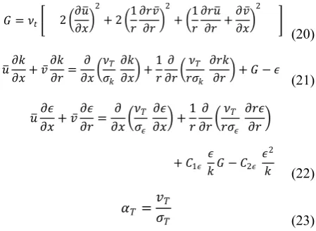
� � �� 2 �

��

2

� 2 �1_��̅_{�� }2� �1_��_{�� }��̅_��2

� (20)

�� ̅ �� 1 � � ��

�� ₍₂₁₎

�� ̅ �� 1 � � ��

� �1� � � � �� 2�

�2

� (22)

��

�� (23)

σT is named as turbulence Prandtl number or Schmidt

number and it was shown that its value is nearly constant by means of experiments. 0.9 is reported as an appropriate value. However it is also stated that the coefficient is affected by buoyancy and streamline curvature. If the RANS equations are re-written by using turbulence viscosity and turbulence diffusion coefficient

for k-ϵ model;

�� ̅ �� 1 � �� 1 � � ��

�2_��

��2� �

� 1 � � �� 1 � �� ̅ �� 2

��

�� ₍₂₄₎

��̅_{�� ̅}��̅_{�� }1_��_{�� }_{�� }� 1_��̅�_{�� }�_��2�̅₂�

� 1 � � �� 2 � ��̅ �� 1 � �� ̅

�� ₍₂₅₎

�� ̅ ��

�� _{�� }1_�_{�� }� �� _�� (26) As summarized above, this work will be conducted by an in-house developed code. In order to narrow the starting range of investigation and validate results comparatively, a series of preliminary analyses is targeted by utilizing commercial codes and/along with open sourced codes. As a first step, present paper contains CFD results of a case using Ansys CFD. Details are given below.

The Ansys CFD analysis is two dimensional and axisymmetric. So the flow domain was drawn as a rectangle after the settings of Ansys Geometry was set to “2D”. A schematic drawing of the geometry is given in Fig. 1.

Fig. 1. Schematic view of the geometry and flow domain

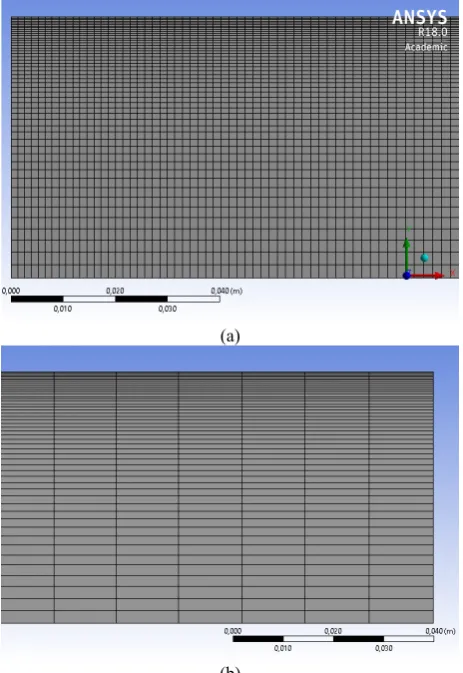
The grid (mesh) was constituted by 20,000 (50x400) quadrilateral cells. 50 cells were located at the inlet along the radius and 400 cells were located at the symmetry along the symmetry axis. A bias was applied to all edges of the geometry by “edge sizing” option in a way that the cell number for an edge stays constant but the edge length of the cell on the edge of the geometry stretches towards symmetry axis and outlet by the bias factor of 10. A “face mesh” option was also applied to have a structured mesh. The node number of the mesh is

20,451. Maximum mesh skeweness is 1.31x10-10_which

can be viewed a success of the structural mesh. The view of the inlet and outlet parts of the mesh is given in Fig.3. In order to asses if the mesh is adequate for the solution, the element number at x and y axes are doubled and halved without touching the bias factors and face meshing of the structural mesh. At this point, 5,000, 80,000 and 320,000 elements were tried. Table 1 shows five different results at the outlet of the pipe for four different element number values. Figure 2 also given for a comparison of different element numbers. According to the results, 80,000 element number was chosen for the comparison of the viscous flow models since tradeoff between time cost and change in turbulent values is satisfactory.

Table 1. Grid comparison - k-ϵ Re=10,000 at pipe outlet 5,000 20,000 80,000 320,000 Vel. (m/s) 0.1219 0.1091 (10%) 0.1041 (4.5%) 0.0942 (9.5%) Tot. Pres. (Pa) 7.45 5.95 (20%) 5.42 (9%) 4.44 (18%)

Turb. Int. 0.1362 0.3494 (156%) 0.443 (26%) 0.4385 (1%)

Turb. Vis.

(5)

5,000 20,000 80,000 320,000

Fig.

2.

C

om

pa

ris

on

o

f d

iff

er

en

t m

es

h e

le

m

en

t n

um

be

r r

es

ul

ts

fo

r

k-ϵ

at R

e=10

,000

u

- x

u

- y

y+

- x

Tur.

int

.

x

µT

-

x

(6)

Although element number changes for the grid independency, Figure 3 gives an idea about the structural mesh and the bias factor.

Four viscous flow models were used; Viscous

Laminar, Spalart-Allmaras, k-ϵ and k-ω. Then the

software was run for four different Re numbers; 50,000, 10,000, 5,000 and 1,000 for the selected turbulence model. Five different two dimensional plot were drawn after the computations where it was possible; u velocity versus x axis (or pipe length), u velocity versus y axis (or pipe radius), wall y+ versus x axis, turbulent viscosity versus x axis and turbulent intensity versus x axis. These two dimensional plots were drawn for different line positions; for instance, lines starting at different “y” axis points at the inlet lie towards the outlet parallel to the wall and the symmetry axis were used for the profiles.

(a)

(b)

Fig.3. (a) mesh view at inlet (b) mesh view at outlet

Fluent solver of the Ansys CFD ran for viscous flow models. General setup can be summarized as; 2D, single precision, serial processing, pressure based, axisymmetric and without gravity. Inlet boundary condition was selected as constant velocity in a way that is ensuring the desired Re number according to the pipe diameter. Outlet boundary condition was set to pressure outlet and its value is fixed as 0 Pa gauge pressure. Hybrid initialization was used. Iteration numbers change between 29 and 145. Solution converges in seconds (between 5 and 30 seconds) since 320,000 elements only used once for the grid examination and mainly 80,000

elements were used. Transition Re number (i.e. 5,000 in

this case) caused highest iteration numbers except for

k-ϵ. The highest iteration number was 145 for k-ϵ and

Re=1,000. The least iteration number was 88 for k-ϵ and

Re=50,000. 0.001 was selected as the convergence

criteria for all residuals. ϵ was the last converged

magnitude among k, continuity and velocity components

for k-ϵ. ω was the first to converge for k-ω. “y” velocity

was converge in the order of first two for all models as expected. Most of the time for the analysis was spent for structural mesh and reporting.

CFD-Post was used for the post processing. The 3D view of the 2D flow domain in CFD-Post is given in Figure 4.

Fig.4. 3D view of the 2D flow domain in CFD-Post

3 Results

(7)

k-ϵ k-ω Spalart-Allmaras Viscous Laminar

Fig.

5.

C

om

pa

ris

on

o

f f

ou

r v

is

co

us

fl

ow

m

od

el

s a

t R

e=

10

,0

00

u

- x

u

- y

y+

- x

Not Available

Tur.

int

.

x

Not Available Not Available

µT

-

x

(8)

At the first glance to Fig. 5, k-ϵ does not yield too distinguished profiles comparing to the remaining models. The range in velocity magnitude considering all profiles is the least for viscous laminar (VL) model

while k-ω and Spalart-Allmaras (S-A) model follow it

respectively. k-ϵ profiles here have the widest range

indicating that this model distinguish more from the VL

for Re=10,000. Actually the models other than k-ϵ imply

a higher Re number comparing to profiles of k-ϵ or in

other words vice versa. Turbulent flow develops faster

than laminar flow due to the presence of turbulent structures that have much more impact on the flow than the molecular viscosity. The boundary layer rises and is restricted because of the turbulent momentum transfer. In the absence of such momentum transfer, the boundary layer of the laminar flow rises slowly with length towards the center. Since more length is needed for the laminar flow development, the initial part of the developing laminar flow looks like a turbulent one. This is the case here because the length of the pipe is 2 m and it is well known that practically development length is

10 Dh for turbulent flows, meaning that 1 m in the

present case. 50 m is needed for the laminar developed flow. It is interesting to see that the velocity profiles for “u” is similar that of VL model and current turbulence models for the turbulence entrance region. One can propose that physical phenomena that are related to “u” component can benefit from the ease of the VL model for the turbulence entrance region.

The k-ϵ developed a thicker boundary layer before

remaining models, yet its velocity profile changes smoothly after a distance more close to the 1 m length. This statement is justified by looking at the “y”=0.045 profile (purple colored). It can be inferred that some of the flow energy is converted into turbulence and hence

velocity profile develops faster for k-ϵ than remaining

models. u-y profiles show identical inlet velocity profiles

for four models. At the outlet, however, VL velocity profile shows that only a big portion has the same velocity magnitude and the maximum magnitude deviates only about 0.003 m/s from the initial velocity magnitude while this value is between 0.003-0.005 for

S-A, 0.004-0.006 for k-ω and 0.007-0.01 for k-ϵ.

Wall treatment in numerical investigation considers y+ dimensionless length. Since VL doesn’t give this information, only wall y+ values of remaining turbulence models along the pipe length are given in Fig.5. This value is calculated for the cell next to the wall. y+ is

desired about 1 for k-ϵ and below 1 for k-ω according to

the literature. Fig. 5 shows that wall y+ is about 0.6 for

k-ϵ and k-ω. For lower mesh element numbers, y+ gets

higher values. Although the turbulent flow can be modeled, there is a region close to the wall where viscous effects become stronger and flow behaves like laminar. The molecular viscosity here plays the major role. This region is characterized by y+ value which is a dimensionless distance. It is defined as “y” times the friction velocity over kinematic viscosity. y+ between 0-6 indicates viscous sub-layer where u+ is equal to y+. 0- 6-30 indicate buffer zone and 6-30-500 is the log-law zone. In the viscous sub-layer, the fluctuating velocity

components diminish and shear stress is only due to the viscosity. The wall functions to be used are determined by looking to y+. Also development of y+ along the perpendicular axis gives information about the development of the boundary layer. Considering above mentioned facts, wall y+ is expected between 0-6.

More turbulent viscosity values are calculated with

k-ϵ than the remaining models which means fluctuating velocity components have higher magnitudes over the flow domain. This should be due to the approach in

which turbulent viscosity is calculated. Again k-ϵ is

found favorable here because it reveals more information about the turbulence comparing to other models.

Turbulence intensity was estimated as 5% at the inlet

for the initial conditions of the simulation. k-ϵ yields

turbulence intensity values greater than 5% along the

pipe length while k-ω yields results implying that

turbulence diminishes with length and becomes weaker. Still, it is understood that a big portion of the flow field

has turbulence intensity value about 5% in k-ϵand 4% in

k-ω. Near the wall, turbulence intensity has values as

high as 15% for k-ϵand 6% for k-ω.

Figure 6 is given for comparison of different

Reynolds numbers considering that k-ϵ is the turbulence

(9)

Re=50,000 Re=10,000 Re=5,000 Re=1,000

Fig.

6.

Compar

ison of four

diff

er

ent R

e numb

ers

for

k-ϵ

u

- x

u

- y

y+

- x

Tur.

int

.

x

µT

-

x

(10)

4 Conclusions

This work aims to declare an ongoing PhD work and its foundation. The motivation of the work is tried to be explained by a literature timeline. The governing equations in 2D cylindrical coordinates are given. Then a preliminary computational fluid dynamics analysis is reported in this paper for a similar turbulent pipe flow case. Ansys CFD commercial software is utilized and four different viscous flow models were compared.

Finally k-ϵ turbulence model results for four different

Reynolds numbers are presented. Following remarks can be drawn from the text.

 The u-y velocity profiles show that the turbulent

flow develops after 10 hydraulic diameters as an experimental justification of the results.

The increase in mesh element number yield

unfavorable results after a certain level and it is thought that this is due to the very small lengths leading to numerical errors. The information of free stream turbulence is also decreasing with increasing mesh element number.

k-ϵ yields more information about the turbulence considering the whole of the flow domain.

k-ω can be preferred if near wall region is specifically important.

 The models don’t make a significant difference in

time cost of the simulation.

 Mesh (grid) elements between 20,000 and 80,000

elements are found favorable for a similar case for further analyses.

Although the method and the findings are related with CFD, experimental results and facts both establish a basis for justification and provide data for developing

modeling. For instance, u-y velocity profiles of the

viscous flow models of the present study is compared to the practical flow development length of turbulent flows in reality which was experimentally obtained in the past. Also it is known that the CFD is used for phenomena that are hard to be measured but in the light of experimentally obtained experimental boundary conditions.

Deeper parametrical analyses of the computational events related to the results will be done in the future for a deeper understanding of the turbulence modeling. Also it is planned to establish a laboratory setup that can enable justification of CFD results by hotwire measurements, led type PIV and thermal camera applications.

Acknowledgment

The academic license of the software used in this work is belonged to Selcuk Univertsity. Authors also would like to acknowledge the financial support of Selcuk University Scientific Research Projects Coordination Unit for the conference participation (project no: 17701387).

References

1. S. Bilir, Selcuk University, Natural and Applied

Sciences Ins., PhD Thesis, Konya, TURKEY (1988)

2. S. Bilir, Int. J. Heat Mass Transfer., 38, 9 (1995)

3. S. Bilir, International Journal of Heat and Mass

Transfer, 45 (2002)

4. S. Bilir, A. Ates, International Journal of Heat and

Mass Transfer, 46 (2003)

5. A. Ates, Selcuk University, Natural and Applied

6. A. Ates, S. Darici, S. Bilir, International Journal of

Heat and Mass Transfer, 53 (2010)

7. S. Darici, Selcuk University, Natural and Applied

8. S. Darici, A. Ates, S. Bilir, J. Fac.Eng.Arch. Selcuk

Univ., 20, 3 (2005)

9. S. Darici, A. Ates, S. Bilir, Journal of

Selcuk-Technic, 7, 2 (2008)

10. S. Darici, S. Bilir, A. Ates, International Journal of

Heat and Mass Transfer, 84 (2015)

11. A.H. Altun, Selcuk University, Natural and Applied

12. A.H. Altun, S. Bilir, A. Ates, International Journal

of Heat and Mass Transfer, 92 (2016)

13. H. Demirpolat, Selcuk University, Natural and

Applied Sciences Ins., PhD Thesis, Konya, TURKEY (2015)

14. S.U. Atmaca, Selcuk University, Natural and

Applied Sciences Ins., PhD Thesis, Konya, TURKEY (2013)

15. S. Sen, Selcuk University, Natural and Applied

16. S. Sen, S. Darici, Applied Thermal Engineering, 111

(2017)

17. N. Kasagi, A. Kuroda, M. Hirata, J. Heat Transfer,

111,2 (1989)

18. Y. Cao, A. Faghri, J. Heat Transfer, 114,4 (1992)

19. W. Jaeger, Nuclear Engineering and Design, 319

(2017)

20. I. Tiselj, R. Bergant, B. Mavko, I. Bajsic, G.

Hetsroni, J. Heat Transfer, 123 (2001)

21. I. Tiselj, L. Cizelj, Nuclear Engineering and Design,

(2012) DOI: 10.1016/j.nucengdes.2012.08.008

22. D.A. Anderson, J.C. Tannehill, R.H. Pletcher,

Computational Fluid Mechanics and Heat Transfer, McGraw-Hill (1984)

23. W.P. Jones, B.E. Launder, Int. J. Heat Mass

Transfer, 15 (1972)

24. B.E. Launder, D.B. Spalding, Comput. Meth. Appl.