via Vertex Separators for Algebraic
Cryptanal-ysis and Mathematical Applications
Kenneth Koon-Ho Wong, Gregory V. Bard and Robert H. Lewis
Abstract. We present a novel approach for solving systems of polynomial equations via graph partitioning. The concept of a variable-sharing graph of a system of polynomial equations is defined. If such graph is disconnected, then the system of equations is actually two separate systems that can be solved individually. This can provide a significant speed-up in computing the solution to the system, but is unlikely to occur either randomly or in applications. However, by deleting a small number of vertices on the graph, the variable-sharing graph could be disconnected in a balanced fashion, and in turn the system of polynomial equations are separated into smaller ones of similar sizes. In graph theory terms, this process is equivalent to finding balanced vertex partitions with minimum-weight vertex separators.
The techniques of finding these vertex partitions are discussed, and ex-periments are performed to evaluate its practicality for general graphs and systems of polynomial equations. Applications of this approach to the QUAD family of stream ciphers, algebraic cryptanalysis of the stream cipher Triv-ium and its variants, as well as some mathematical problems in game theory and computational algebraic geometry are presented. In each of these cases, the systems of polynomial equations involved are well-suited to our graph partitioning method, and constructive results are discussed.
Mathematics Subject Classification (2000).05C90, 11T71, 68R10, 94A60, 14G50.
Keywords.balanced vertex partitions, graph partitioning, polynomial systems of equations, QUAD, Trivium, resultants, algebraic cryptanalysis.
1. Introduction
a finite element mesh across nodes in parallel computations [54]. These techniques primarily focus on linear systems over the real or complex fields. In this paper, we apply similar graph theory techniques to systems of multivariate polynomial equations, and develop methods of partitioning these systems into ones of smaller sizes via their “variable-sharing” graphs. These techniques are intended to work over any field, finite or infinite, but are particularly suited to GF(2) for use in algebraic cryptanalysis of symmetric ciphers.
Computing the solution to a system of multivariate polynomial equations is an NP-complete problem [7, Ch. 3.9]. A variety of solution techniques have been developed for solving these polynomial systems over finite fields, such as lineariza-tion, Gr¨obner bases, and resultants [8, Ch. 12], as well as recent ones such as SAT-solvers [9] and the Raddum-Semaev method [60]. Over the real and complex numbers, numerical techniques are also known including Gradient Descent, New-ton’s Method, the Conjugate Gradient Methods and the Nelder-Mead Simplices Algorithm [6]. In addition, homotopy methods, also known as continuation meth-ods, have become popular [3], but require the field to be ordered and complete. The graph partitioning method introduced in this paper could be a novel addition to the variety of methods available, principally as a preprocessor.
From a multivariate polynomial system of equation, a variable-sharing graph is constructed with a vertex for each variable in the system, and an edge between two vertices if and only if those variables appear together in any equation in the system. Clearly, if the graph is disconnected, the system can be split into two separate systems of smaller sizes, and they can be solved for individually. However, even if the graph is connected, we show that it may be possible to disconnect the graph by eliminating a few variables by, for example, guessing their values when computing over a small finite field, and thereby splitting the remaining system. Over larger and infinite fields, we show how to perform the elimination with resultants. This suggests a divide-and-conquer approach to solving systems of equations. When the polynomial terms in the an system of equations are very sparse, we show that the system can usually be reduced to a set of smaller systems, whose solutions can be computed individually in much less time.
In order for a partition of a system to be productive, the minimum number of variables should be eliminated, and the two subsystems must be approximately equal in size. This ensures that the benefit of partitioning the system is maximised. These conditions lead to the problem of finding a balanced vertex partition with a minimum-weight vertex separator on its variable-sharing graph, which is an NP-complete problem [39, 55]. Nevertheless, heuristic algorithms can often find near-optimal partitions efficiently [41]. In this paper, we apply this approach to polynomial systems arising from algebraic cryptanalysis of ciphers, and achieve sig-nificant advantages in attacking these ciphers. We also discuss some uses of graph partitioning to solve mathematical problems in game theory and computational algebraic geometry more efficiently.
into ones of smaller sizes using graph partitioning methods. Sections 3.1 and 3.2 describe how the actual partitions can be found. In GF(2) polynomial systems, the values of the variables to be removed can be simply guessed, but in larger or infinite fields, we present an alternative method in Section 3.3. Section 4 provides results for some partitioning experiments and analyses the feasibility of equation solving via graph partitioning methods.
We offer two cryptographic applications of vertex parititioning in Section 5. The first is a method whereby a manufacturer of a sparse implementation of QUAD, a provably-secure stream cipher family, could “poison” the polynomial system in the cipher, and thereby enable messages transmitted with it to be read by the manufacturer. Second, we present an algebraic cryptanalysis of Trivium, a profiled stream cipher in the eSTREAM project, as well as its reduced ver-sions Bivium and Bivium-A, and discuss their vulnerability or resistance to graph partitioning methods.
We also offer two applications to other branches of mathematics in Section 6. The first is finding the Nash equilibria in an 8-player game called “the cube game”. Normally, the equations for p-player Nash equilibria, without coalitions, are of degree (p−1) [23, 63]. In this case, the equations are cubic, and the solution of them is greatly sped up by the techniques from this paper. The second is the Apollonius Problem, known to the Ancient Greeks but used in molecular chemistry [49].
Conclusions will be drawn in Section 7. Appendix A discusses the NP-completeness of finding balanced graph partitions. Some theorems guaranteeing the existence of balanced graph partitions for special graphs are given in Appendix B. An algo-rithm to convert from edge partitions to vertex partitions is given in Appendix C. Finally, some additional experimental results of graph partitioning are presented in Appendix D.
2. Preliminaries
In this section, a brief introduction to graphs and graph partitioning is presented. For a detailed treatment on graph theory, see [36]. A graph describes a set of nodes and connections between them. Each node is called a vertex, and a connection between two nodes is called an edge.
LetG= (V, E) be a graph with vertex setV and edge setE. Two vertices vi, vj ∈ V are connected if there is a path from vi to vj through edges in E. A
disconnected graph is a graph where there exists at least one pair of vertices that is not connected, or if the graph has only one vertex.
A graphG1= (V1, E1) with vertex setV1⊆V and edge setE1⊆Eis called a
subgraph ofG. Given a graphG, subgraphs ofGcan be obtained by removing ver-tices and edges fromG. LetG= (V, E) be a graph withkvertices andledges, such that V ={v1, v2, . . . , vk−1, vk},E={(vi1, vj1),(vi2, vj2), . . . ,(vil, vjl)}. Removing
andE1 ={(vi, vj)∈E|vk ∈ {/ vi, vj}}. We callG1 the subgraph ofGinduced by
the vertex set (V − {vk}).
Let G1 = (V1, E1), G2 = (V2, E2) be two subgraphs of G. G1, G2 are
con-sidered disjoint if no vertices inG1 are connected to vertices in G2. Clearly, the
conditionV1∩V2=∅is necessary.
2.1. Graph Connectivity
The goal of partitioning a graph is to make the graph disconnected by remov-ing some of its vertices or edges. The number of vertices or edges that needs to be removed to disconnect a graph is related to its vertex or edge connectivities respectively.
Definition 2.1. Thevertex connectivity κ(G) of a graphGis the minimum number of vertices that must be removed to disconnect G. The edge connectivity λ(G) of Gis the minimum number of edges that must be removed to disconnectG.
Clearly, a disjoint graph has vertex connectivity zero. On the other extreme, a complete graphKn, where allnvertices are connected to each other, has vertex
connectivity (n−1). The removal of all but one vertex fromKn results in a graph
consisting of a single vertex, which is considered to be disconnected.
The following theorem relates graph connectivities with paths in the graph.
Theorem 2.2 (Menger[53], 1927). If a graph hasnvertex-distinct paths from any particular vertex to any other, then its vertex connectivity is at least n. Further-more, if there aren edge-distinct paths then its edge connectivity is at leastn.
2.2. Graph Partitioning
The process of removing vertices or edges to disconnect a graph is called vertex partitioning or edge partitioning respectively. All non-empty graphs admit trivial vertex and edge partitions, where all connections to a single vertex are removed. This is obviously not useful for most applications. In this paper, we only consider balanced partitions with minimum-weight separators, in which a graph is separated into subgraphs of roughly equal sizes by removing as few vertices or edges as possible.
2.2.1. Balanced Vertex Partitions. More specifically, our primary focus of this paper is on balanced vertex partitions.
Definition 2.3. LetG= (V, E) be a graph. A vertex partition (V1, C, V2) ofGis a
partition ofV into mutually exclusive and collectively exhaustive sets of vertices V1, C, V2, where V1, V2 are non-empty, such that no edges connect vertices ofV1
directly to vertices ofV2. The removal of C causes the subgraphs induced by V1
andV2to be disjoint, henceC is called the vertex separator.
For a balanced vertex partition, we requireV1andV2to be of similar size. For
Definition 2.4. LetG= (V, E) be a graph, and (V1, C, V2) be a vertex partition of
Gwith vertex separator C (see Definition 2.3). If max(|V1|,|V2|)≤α|V|, thenG
is said to have anα-vertex separator.
The problem of findingα-vertex separators is known to be NP-hard. For more details, see Appendix A.
Definition 2.5. LetG= (V, E) be a graph. If (V1, C, V2) is a vertex partition ofG,
then define
β= max(|V1|,|V2|) |V1|+|V2|
=max(|V1|,|V2|) |V| − |C| to be a measure of balance of the vertex partition.
Suppose the balance of a vertex partition ofGinto (V1, C, V2) isβ=α, then
the partition also satisfies max(|V1|,|V2|) =α(|V1|+|V2|)≤α|V|, and hence theG
has anα-vertex separator. Therefore, theorems that apply toα-vertex separators would also apply to vertex partitions with balanceα. See [55] for more details ofα -vertex separators. Several theoerems governing the existence ofα-vertex separators are presented in Appendix B.
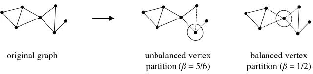
Figure 1 presents examples of balanced and unbalanced partitions, and their respective β values. The vertex separators C are circled, with the partitioned vertices V1, V2 outside. The removal of the vertices in the separators disconnects
the graphs. For a balanced partition,β should be close to 1/2.
unbalanced vertex partition (ȕ= 5/6)
balanced vertex partition (ȕ= 1/2) original graph
Figure 1. Balanced and Unbalanced Vertex Partitions
2.2.2. Partitioning Algorithms and Software. Balanced edge partitioning is widely used in scientific and engineering applications, such as electric circuit design [62], parallel matrix computations [44], and finite element analysis [54]. Software pack-ages are readily available for computing balanced edge partitions using a variety of algorithms [10, 13, 31, 37, 56, 57, 66].
Unless otherwise stated, from here on we will only consider the problem of balanced vertex partitioning with minimum-weight vertex separators (sometimes simply referred to as vertex partitioning or partitioning) and its applications to solving systems of multivariate polynomial equations.
3. Partitioning Polynomial Systems
In this section, our method for partitioning systems of multivariate polynomal equations by finding balanced vertex partitions of their variable-sharing graphs is described. Several methods for finding and using these partitions will also be discussed.
Definition 3.1. LetF be the polynomial system
f1(x1, x2, . . . , xn) = 0
f2(x1, x2, . . . , xn) = 0
.. . fm(x1, x2, . . . , xn) = 0
of m polynomial equations in the variables x1, x2, . . . , xn. The variable-sharing
graph G= (V, E) of F is obtained by creating a vertex vi ∈V for each variable
xi, and creating an edge (vi, vj)∈E if two variablesxi, xj appear together in any
polynomialfk.
Example 3.2. Suppose we have the following quadratic system of equations over GF(2), where the variablesx1, x2, . . . , x5are known to take values in GF(2).
x1x3+x1+x5= 1
x2x4+x4x5= 0
x1x5+x3= 0
x2x5+x2+x4= 0
x2+x4x5= 1
(1)
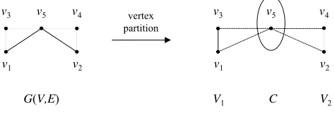
The corresponding variable-sharing graph G and a balanced vertex partition is shown in Figure 2.
The quadratic system can then be partitioned into two systems of equations with the common variablex5 as follows.
x1x3+x1+x5= 1 x2x4+x4x5= 0
x1x5+x3= 0 x2x5+x2+x4= 0
x2+x4x5= 1
v4 v3
v2 v1
v5 v3 v4
v2 v5
v1
V1 C V2
G(V,E)
vertex partition
Figure 2. Graph of quadratic system (1) and a vertex partition.
Sincex5∈GF(2), we can substitute all possible values ofx5into (1) and computing
solutions to the reduced systems to give
x5= 0⇒no solution
x5= 1⇒x= (1,0,1,0,1)
The solution obtained is the same as if we had directly computed the solution to the full system of equations. However, the systems have been reduced to having less than half the number of variables compared to the the original, at the cost of applying guesses to one variable.
This method of guessing and solving will be used for the algebraic crypt-analysis of the Trivium stream cipher in Section 5. For simplicity, from here on we might use the terms for variables and vertices interchangeably to denote the variables in the polynomial systems of equations and their corresponding vertices in the variable-sharing graphs, provided there are no ambiguities.
3.1. Special Cases for Low Vertex-Connectivity
LetG= (V, E) be a variable-sharing graph representing a polynomial system of equations. The special case of a disconnected graph with vertex connectivityκ= 0 for a graphGcan be detected with a standard Depth-First Search (DFS). Mark each vertex “unvisited” initially, and mark it “visited” as the DFS progresses. If not all nodes are visited by the end of the DFS, then G is not connected. This has expected running time of Θ(|V|d) if the average degree of the graph is d. In this case, the polynomial system can be partitioned trivially, without a need to compute a vertex separator.
The special case of κ= 1 can be detected by removing and restoring, one at a time, all vertices, and checking a DFS in each case. Likewise, κ= 2 can be detected by removing all possible pairs. The number of steps required to detect a vertex-connectivity of at mostk is
k X
i=0
µ|
V| i
|V|d ≈ (|V|+ 1−k/2)
k+1
d
where we have used
µ
a b
+
µ
a b−1
=
µ
a+ 1 b
,
µ
a n
≈ (a−n/2)
n
n! , n≪a.
This approach also has the advantage of revealing the vertex separator. We call this Pseudo-Brute Force Search. For example, if |V| = 100, testing up toκ = 7 requires
7
X
i=0
µ
100 i
= 17,278,988,696
depth-first searches. This may still be a feasible computation on distributed com-puting systems, since each DFS can be performed independently of each other.
Since we desire a balanced partition, we can mark each subset ofk or fewer vertices that partitions the graph, found during the search, with a difficulty num-ber. The difficulty number should be the size of the largest connected component, since this will presumably be the hardest subsystem of equations to solve. At the conclusion of the search, we take the partition with the lowest difficulty number. This would assure that the optimal partition of all those possible can be discovered.
3.2. Heuristic Partitioning Algorithms
The method above does not scale up to large graphs with high vertex connectiv-ities, so other computational methods are required. While balanced partitioning is an NP-hard problem, a variety of heuristic algorithms have been found to be very efficient in finding near-optimal partitions. Software implementing these al-gorithms and their applications are as discussed in Section 2.2.2.
One of the efficient schemes for balanced graph partitioning is called multi-level partitioning, which we have selected to use for our experiments. Suppose a graph G0 is to be partitioned. Firstly,G0 “coarsened” progressively into simpler
graphs G1, G2, . . . , Gr by contracting adjacent vertices. The process of choosing
vertices for contraction is called matching. After reaching a graph Gr with the
desired level of simplicity, a partitioning is performed. The result is then pro-gressively refined back through the chain of graphs Gr−1, Gr−2, . . . , G0. At each
refining step, a refinement to the partition can be performed. The output is then a partition ofG0. Details of multilevel partitioning can be found in [38, 41].
Exam-ples of partitioning and refinement algorithms include the ones by Kerighan-Lin [42] and Fiduccia-Mattheyses [30].
software requirements for finding balanced vertex partitions. These will be used for the experiments in Section 4 and for the algebraic cryptanalysis of Trivium in Section 5.2.
3.3. Exploting Partitions in Large Finite Fields or Infinite Fields
As shown at the start of this section, for a polynomial system over GF(2), a partition is easy to exploit. There are only 2|C|possible values for all the variables in the vertex separator |C|. Since solving the two smaller systems of equations is much faster than solving the original system, provided that the partition is balanced and C is relatively small, it is feasible to check every possibility of the values of the variables in C. If we were to partition equations in, for example GF(256) or GF(16), as used in the Advanced Encryption Standard [22] and one of its variants [61] respectively, then the number of possibilities to check for|C| variables in the vertex separators would be 256|C| and 16|C| respectively, which would be extremely infeasible. In these cases, and for the case of an infinite field likeQ, we suggest the following method.
Suppose the variablesV in a system of polynomial equations are partitioned intoV1, V2 with vertex separatorC, and the system is then divided into two
sub-systems F, G with variablesV1∪C andV2∪C respectively. This means that, in
each of the subsystems, there are no equations having a variable fromV1 and also
a variable fromV2. Now relabel the variables as follows. Denote the variables
rep-resented by vertices inCbyxi, those fromV1asyi, and those inV2aszi. Also, let
the equations inF befi, those inGbe gi. Then, we can use a well-known
tech-nique of resultants, whereby unknowns are divided into two classes: “variables” and “parameters”. Given mpolynomials, one can label (m−1) of the unknowns as “variables”, and the remaining unknowns as “parameters”. The resultant of these mpolynomials will be a polynomial entirely in the “parameters”, but with none of the “variables”. This is a highly-non-trivial process, but form <12 it is quite feasible. This can be repeated for all subsets of sizemamong the equations. As stated before, there are two sets of equations, namely fi, gi. Let xi be
the “variables” in both sets, and yi, zi be the “parameters” in their respective
sets. We can then take |C|+ 1 equations from fi, and calculate their resultant.
This will be a polynomial entirely in terms ofyi. This can then be applied to all
collections offi consisting of exactly |C|+ 1 equations, or only some collections,
as desired. This process will also be performed for the collections of size |C|+ 1 among gi, to produce polynomials entirely in terms of zi. Observe now that the
resultants obtained are entirely disjoint, and can be solved for separately. Their solutions can then be substituted back into the original polynomials to obtain the “variables”xi. Note that this technique requires min(|V1|,|V2|)>|C|, preferably
4. Experiments
To evaluate the practicality of partitioning large systems of equations, experi-ments have been performed on random graphs of different sizes resembling typical variable-sharing graphs. These experiments were run on a Pentium M 1.4 GHz CPU with 1 GB of RAM using the Meshpart [34] Matlab interface to the Metis [40] partitioning software.
Definition 4.1. LetG= (V, E) be a graph. Thedegree deg(v) of a vertexv∈V is the number of edgese∈E incident (connecting) tov.
Definition 4.2. Thedensity ρ(G) of a graphG= (V, E) is the ratio of the number of edges|E|in Gto the maximum possible number 1
2|V|(|V| −1) of edges inG.
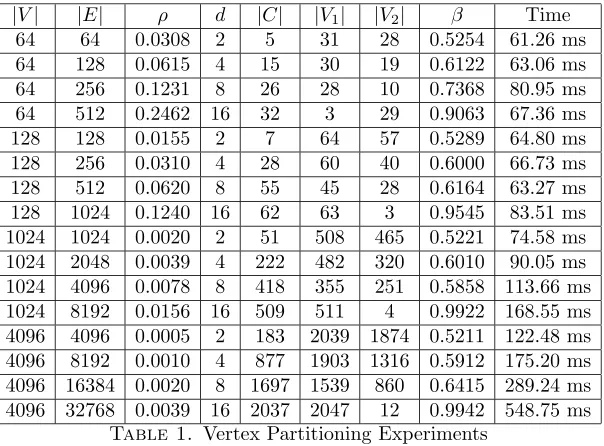
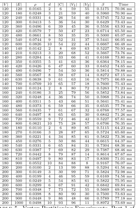
In each experiment, random graphs G = (V, E) are generated, each with prescribed number of vertices|V|, number of edges|E|, and average degreedof its vertices. Their densitiesρare also computed. For each graph, a vertex partition is performed to give (V1, C, V2), whereCis the vertex separator. The balance measure
βis then computed, and the time required is also noted. Some experimental results are shown in Table 1. More results can be found in Tables 4-5 in Appendix D.
|V| |E| ρ d |C| |V1| |V2| β Time
64 64 0.0308 2 5 31 28 0.5254 61.26 ms 64 128 0.0615 4 15 30 19 0.6122 63.06 ms 64 256 0.1231 8 26 28 10 0.7368 80.95 ms 64 512 0.2462 16 32 3 29 0.9063 67.36 ms 128 128 0.0155 2 7 64 57 0.5289 64.80 ms 128 256 0.0310 4 28 60 40 0.6000 66.73 ms 128 512 0.0620 8 55 45 28 0.6164 63.27 ms 128 1024 0.1240 16 62 63 3 0.9545 83.51 ms 1024 1024 0.0020 2 51 508 465 0.5221 74.58 ms 1024 2048 0.0039 4 222 482 320 0.6010 90.05 ms 1024 4096 0.0078 8 418 355 251 0.5858 113.66 ms 1024 8192 0.0156 16 509 511 4 0.9922 168.55 ms 4096 4096 0.0005 2 183 2039 1874 0.5211 122.48 ms 4096 8192 0.0010 4 877 1903 1316 0.5912 175.20 ms 4096 16384 0.0020 8 1697 1539 860 0.6415 289.24 ms 4096 32768 0.0039 16 2037 2047 12 0.9942 548.75 ms
Table 1. Vertex Partitioning Experiments
n is O(n2), the edge density must be smaller with a larger graph for practical
partitions. This is a reasonable assumption for polynomial systems, since certain sparse systems have only a small number of variables in each equation, regardless of the total number of variables in the system. This fact is true for the case of Trivium in Section 5.
It is also noted that the time required to compute vertex partitions are quite short for the graph sizes considered, and would be negligible compared to the time required to solve the partitioned systems.
4.1. Predictingβ
Figure 3 shows the effect of varying the number of edges in a graph on the balance β of vertex partitions for graphs of different sizes, where n=|V|. Each value of the partition balance parameterβ shown in the figure is the average value of 200 separate graph partitions.
2 3 4 5 6 7 8 9 10
0.5 0.55 0.6 0.65 0.7 0.75 0.8 0.85 0.9
Average Degree (d)
α
n = 50 n = 100 n = 150
Figure 3. Partition Balance vs Average Degree of Graph
It can be observed that the balance parameter β increases approximately linearly with the average degreedof the graphs. Furthermore, the increase seems to be slower with graphs having more vertices. However, Table 1 suggests that the increase becomes faster again for even larger graphs. From the vertex partition theorems shown in Appendix B, we assert that a reasonable balance is obtained when 1
2 ≤ β ≤ 2
3. With the graph sizes considered in Figure 3, it seems that
this reasonable balance can be obtained with d≤6. This also means that when d ≤ 6, the graph may be planar, since planar graphs has 2
3-vertex separators,
which implies 1 2 ≤β ≤
2
3. Marginally balanced partitions withβ < 3
4 are possible
Based upon the graph shown in Figure 3, an experiment is performed to try to predictβ as a function of the number n of vertices and average degreed. An extended dataset for 25≤n≤400 and 2≤d≤10 with a total of 192 data points were used to arrive at the prediction. The following formula with 8 coefficients was found using a power-law regression.
β≈0.008369149n−0.778855746
d2.584865649
+ 2.489035921e−0.246287194d
+ 12.33556203−14.06086217d−0.074824899
The data and predictions are provided in Tables 6-8 in Appendix D. The prediction has an average relative error of 1.90%, and a maximum error over the data set of 6.76%.
5. Applications to Algebraic Cryptanalysis
A bit-based stream cipher usually consists of an internal state s ∈ GF(2)n and
a defined procedure to updates at each timestept of the cipher. At the start of an encryption, a key initialisation phase would take place, whereby a secret keyk and a known initialisation vectorIV are used to set itssto its secret initial state s0. The cipher then begins its keystream generation phase, and outputs a series of
keystream bitsz1, z2, . . . from sat each timestep t, wheres is updated based on
the defined procedure. This procedure can usually be described byst+1 =g(st)
at each timestep t. Simliarly, the keystream bits zt can usually be described by
zt = f(st) at each timestep t. Given plaintext bits p1, p2, . . ., the stream cipher
encrypts them using the keystream into ciphertext bits c1, c2, . . . as ct =pt+zt
over GF(2).
Since stream ciphers are traditionally designed for implementation in digital circuits, f, g can often be represented as polynomial functions. Then, if both pt
andctare known for enough timesteps, one can write a system of equations based
onzt=pt+ctusingf, g. This forms the foundation of algebraic cryptanalysis. To
perform an algebraic cryptanalysis of a stream cipher, the cipher is first described as a system of equations. Its variables usually correspond to the bits in the key k or the initial state s0. If the variables are from k, solving the system is called
“key recovery”, and the cipher is immediately broken. If the variables are froms0,
solving the system is called “state recovery”, and the key could be derived from the solution, whose difficulty depends on the specific cipher design.
equations arising from the cipher, and refer the reader to the respective references of these ciphers for their design and implementation details.
5.1. QUAD
The stream-cipher family QUAD is given in [11]. The security of QUAD is based on the Multivariate Quadratic (MQ) problem. The heart of the cipher is a random system ofkn quadratic equations innvariables over a finite field GF(q). Usually, we haveq= 2, but implementations withq= 2shave also been discussed [69]. This
system of equations is not secret, but publicly known, and there are criteria for these equations, such as those relating to rank, which we omit here. In a different context, QUAD has been analyzed in [69, 5], and [8, Ch. 5.2].
5.1.1. Equations of QUAD. The authors of QUAD recommendk= 2 andn≥160, so it is assumed that we have a randomly generated system of 2n= 320 equations inn= 160 unknowns. The system is to be drawn uniformly from all those possible, which is to say that the coefficients can be thought of as generated by fair coins.
Each quadratic equation is a map GF(2)n→GF(2), so the first set ofn
equa-tions form a map GF(2)n →GF(2)n called f
1, and the second set ofn equations
also form a map of the same dimensions called f2. The internal state is a vector
sof 160 bits. The first 160 equations are evaluated ats, and the resulting vector f1(st) =st+1 becomes the new state. The second 160 equations are evaluated to
become the output of that timestep zt = f2(st). The vector zt is added to the
next n bits of the plaintextpt over GF(2), and is transmitted as the ciphertext
ct=pt+zt. There is also an elaborate setup stage which maps the secret key and
an initialization vector to the initial states0.
Finding a pre-image under the mapsf1, f2 i.e. finding si givensi+1 andzi,
is equivalent to solving a quadratic system of 2nequations innunknowns, and is NP-hard [7, Ch. 3.9]. This is further complicated by the fact that the adversary would not havesi+1, but rather onlyzi+pi.
Given a known-plaintext scenario, where the attacker knows both the plain-textp1, p2. . . , pn and ciphertextc1, c2, . . . , cn, one can write the following system
of equations.
c1+p1 = z1=f2(s1)
c2+p2 = z2=f2(s2) =f2(f1(s1))
c3+p3 = z3=f2(s3) =f2(f1(f1(s1)))
.. . = ...
ct+pt = zt=f2(st) =f2(f1(f1(f1(· · ·f1(
| {z }
itimes
s1)· · ·))))
The interesting fact here is thatf2(f1(f1(· · ·f1(s1)· · ·)))) and higher iterates
might be quite dense even iff1is sparse. The authors of QUAD have excellent
system, which would require a large gate count or would be slow in software. Thus, in their conference presentation but not the paper, the authors of QUAD mention that a slightly sparse f might still be secure. Furthermore, because of repeated iteration and the general difficulty of the MQ problem, there would probably be no feasible algebraic attack against the sparse version.
5.1.2. Poisoned Equations and QUAD. One could imagine the following scenario, which is inspired by Jacques Patarin’s system “Oil and Vinegar” [43]. A malicious manufacturer does not generate the system at random, but rather creates a system that is sparse and has vertex connectivity of 20, for some vertex partition with β ≈ 0.6. Our experiments in Section 4 show that this is a feasible partition. The malicious manufacturer would claim that the system is sparse for efficiency reasons and it might have a considerably faster encryption throughput than a QUAD system with quadratic equations generated by fair coins.
Some separators of 20 vertices divides the variable sharing graph into roughly 56 and 84 vertices. This means that an attacker would need only to know the plaintext and ciphertext of one 160-bit sequence, and solve the equation
f2(f1(f1(· · ·f1(f1(
| {z }
i−1times
s1))· · ·))) =pt+ct
.
For any guess of the key, this would be solving 56 equations in 56 unknowns and 84 equations in 84 unknowns. Such a problem is certainly trivial for a SAT-solver, as shown in [9], [7, Ch. 3] and [8, Ch. 7]. Only 220 iterations would be
required, and with a massive parallel network, such as BOINC [1], this would be quite feasible.
5.1.3. Remedy to Poisoned Systems for QUAD. While finding a balanced vertex partition of a graph Gis NP-hard, as discussed in Appendix A, calculating the vertex connectivity κ(G) is easier. If κ(G) > 80, for example, then there is no vertex partition, balanced or otherwise, with fewer than 80 vertices in the vertex separator. Then, by calculatingκ(G), a manufacturer of QUAD could prove that they are not poisoning the quadratic system as explained in the previous subsec-tion. There are also techniques to generate functions with verifiable randomness [16], which could be used to construct polynomial systems of equations for QUAD, such that they are provably not poisoned.
5.2. Trivium
0 200 400 600 800 0
100
200
300
400
500
600
700
800
900
nz = 25962
Figure 4. Graph Adjacency Matrix of Trivium Equations
Cryptanalytic results on Trivium and Bivium have been presented in [12, 26, 27, 28, 51, 52, 58, 64].
5.2.1. Equation Construction. The equations governing keystream generation from the initial states0 can be found in [25] for Trivium and [59] for Bivium. In the
al-gebraic cryptanalysis presented in this paper, we do not consider the initialisation phase from the key k and initialisation vector IV, and hence we are performing state recovery of the cipher.
Trivium can be described as a system of 288 multivariate polynomial equa-tions in 288 variables, but we found that this is too dense for partitioning to be useful. Instead, we use the quadratic equations presented in [59], which contains more variables, but are very sparse. The quadratic system of Trivium consists of 954 sparse quadratic equations in 954 variables, and observed keystream from 288 clocks. Similarly, the polynomial system of Bivium-A and Bivium-B consists of 399 sparse quadratic equations in 399 variables, and observed keystream from 177 clocks. There are at most 6 variables present in each equation, hence the variable-sharing graph has maximum degree 6, and there is at most one quadratic term in an equation. We attempt to solve these equations via partitioning.
5.2.2. Equation Partitioning. The sparse quadratic equations for Trivium and Bivium are constructed as per [59], and their variable-sharing graphs are then computed. Figure 4 shows the adjacency matrix for the variable-sharing graph of Trivium. The sparsity of this matrix appears promising for a reasonable partition. Graphs for Bivium are of similar sparsity.
Partitioning these variable-sharing graphsG= (V, E) into vertex setsV1, V2
State Number of
Cipher Size Variables |C| |V1| |V2| β
Bivium-A 177 399 96 156 147 0.5149 Bivium-B 177 399 122 150 127 0.5415 Trivium 288 954 288 476 190 0.7147 Table 2. Partitioning Equations of Bivium-A, Bivium-B and Trivium
From these results, it seems that both of the Bivium ciphers admit very balanced partitions, whereas Trivium did not. However, using an implementation of the greedy algorithm in Appendix C, we were able to find a balanced partition for Trivium with |C|= 295 and β ≈0.5. This result is still preliminary, so we omit further details here.
The sizes of the vertex separatorsCare the number of variables that must be eliminated to separate the systems into two. In algebraic attacks, this corresponds to the number of variables whose values are to be discovered or guessed at a complexity of 2|C|. The process of guessing certain bits in order to find a solution is called partial key guessing. If the guessed bits are correct, then solving the remaining system would lead to the solution.
For Trivium, the separator size is exactly the same as the internal state size. For Bivium and Bivium-A, the separator sizes are less than the internal state size, but larger than the key size of 80-bits. This means that the time complexity of partial key guessing on all bits of the separators would be higher than that of a brute force search on the key.
5.2.3. Partial Key Guessing. However, we can attempt to guess less bits then the size of the separator C. The remaining system would not be separated, but it can still be solved. We have found by experiment that a partial key guess on a subset of bits inC provides a significant advantage over that on random bits, in that the reduced polynomials systems are much faster to solve. These experiments were performed using Magma [14] with its implementation of the Gr¨obner basis algorithm F4 [29] for solving the reduced polynomial systems. The results are
shown in Table 3, where n is the number of bits guessed, m is the number of equations resulting from the guess, withqof them being quadratic. Correct guesses are always used to reduce the polynomial systems, which means that the time and memory use presented are for solving the entire system arriving at a unique solution. All values are averaged over at most 10 individual runs.
Cipher All Guesses in|C| n m q Time Memory
Bivium-A No 24 422 193 26 s 42 MB
Bivium-A No 22 419 200 120 s 175 MB
Bivium-A No 20 421 200 195 s 234 MB
Bivium-A No 18 417 203 2558 s 843 MB
Bivium-A Yes 24 422 187 1 s 22 MB
Bivium-A Yes 22 420 190 1 s 22 MB
Bivium-A Yes 20 419 193 45 s 89 MB
Bivium-A Yes 18 417 195 80 s 127 MB
Bivium-A Yes 16 415 201 1101 s 751 MB
Bivium-A Yes 14 413 202 2023 s 1200 MB
Bivium-B No 82 481 140 180 s 1044 MB
Bivium-B No 80 479 143 392 s 1044 MB
Bivium-B No 78 477 146 740 s 1044 MB
Bivium-B No 76 475 141 1213 s 1044 MB
Bivium-B Yes 74 473 128 4 s 35 MB
Bivium-B Yes 70 469 132 12 s 62 MB
Bivium-B Yes 66 465 136 623 s 546 MB
Bivium-B Yes 62 461 141 3066 s 1569 MB
Trivium No 280 1333 329 13 s 80 MB
Trivium No 276 1228 341 110 s 308 MB
Trivium No 272 1224 343 155 s 554 MB
Trivium No 268 1221 344 125 s 576 MB
Trivium No 264 1217 344 594 s 1569 MB
Trivium No 260 1213 344 747 s 3600 MB
Trivium Yes 190 1140 493 14 s 584 MB
Trivium Yes 184 1135 497 16 s 596 MB
Trivium Yes 180 1131 499 18 s 596 MB
Trivium Yes 178 1130 499 18 s 596 MB
Trivium Yes 176 1127 499 4511 s 1875 MB
Trivium Yes 174 1126 501 10543 s 3150 MB
Table 3. Partial Key Guessing on Trivium and Bivium
the time complexity for an attack on Bivium-B is reduced from 278
T to 266
T with the use of the separator, whereT denotes the time complexity required to compute a solution to a reduced system.
about 0.15 seconds to process. This is much faster than the 45 seconds required from the experimental results to process a correct guess.
5.2.4. A Bit-Leakage Attack. There is another scenario whereby the graph parti-tioning would provide an advantage to algebraic cryptanalysis. Suppose by some means, accidental or deliberate, some bits of the internal state could be leaked to an attacker. This would occur in a side-channel attack setting. If the attacker could control which bits are leaked, then the best choices would be those variables in the separator. Fewer bits would need to be leaked before the system of equations can be solved in a reasonable time.
6. Applications to Mathematics
In this section, two applications of graph partitioning to mathematical problems are presented.
6.1. Nash Equilibria
This is a well known topic in economic game theory [23, 63]. Briefly, a strategy is a Nash equilibrium if for each playerpin the game,pcould never attain a better payoff by changing only p’s own strategy, leaving all other strategies fixed. On the other hand, coalitions of players can change their strategies simultaneously to achieve higher payoff.
Nash equilibria can be characterized by systems of polynomial equations [63]. We investigate here a “cube game”, based on a graph Gresembling the edges of the 3-dimensional cube. The eight players are associated to the vertices of the cube. Each player’s name, vertex coordinate in 3-space, and variable is shown as follows.
Alice Bob Carl Dick Fran Gary Hugh Jane
000 001 010 011 100 101 110 111
a b c d f g h j
game discussed by Sturmfels [63], we have these equations: (u1b−1)(u1c−1)(u1f −1) =rr
(u1a−1)(u1d−1)(u1g−1) =rr
(u2a−1)(u2d−1)(u1h−1) =rr
(u2b−1)(u2c−1)(u1j−1) =rr
(u3a−1)(u2g−1)(u2h−1) =rr
(u3b−1)(u2f−1)(u2j−1) =rr
(u3c−1)(u3f−1)(u3j−1) =rr
(u3d−1)(u3g−1)(u3h−1) =rr
(3)
Sturmfels used valuesu1= 3, u2= 5, u3= 7, rr= 1/10.
6.1.1. Experimental Findings. Our first experiments were performed on the ma-chine1
sage.math.washington.eduusing Magma [14] and Singular [35]. The
ma-chine has 64 gigabytes of RAM and 16 AMD Opteron cores. We chose the degree-reversed lexicographical order for the polynomial equations. It is known that Magma uses the algorithm F4 [29], and Singular uses the Buchberger algorithm [15].
Even after substituting in the above constants for u2, u3, and rr, keeping
u1 as symbolic, no solution was found by Magma after 63 minutes, using 585
megabytes of RAM. Neither was a solution forthcoming from Singular after using 1054 megabytes of RAM and 55 minutes.
However, one can see that half the equations use the variables b, c, f, j and the other half usea, d, g, h. Thus we can split the system into
(u1b−1)(u1c−1)(u1f−1) = 1/10,
(u2b−1)(u2c−1)(u1j−1) = 1/10,
(u3b−1)(u2f−1)(u2j−1) = 1/10,
(u3c−1)(u3f−1)(u3j−1) = 1/10,
(4)
which was solved in 0.1 seconds by Magma and 0.15 seconds by Singular, and (u1a−1)(u1d−1)(u1g−1) = 1/10,
(u2a−1)(u2d−1)(u1h−1) = 1/10,
(u3a−1)(u2g−1)(u2h−1) = 1/10,
(u3d−1)(u3g−1)(u3h−1) = 1/10,
(5)
which was solved in 0.1 seconds by Magma and 0.17 seconds by Singular.
Since u1 is a constant known parameter, it can be shared between the two
broken systems. If the parametersu2, u3, andrrare left in the equations, the same
splitting applies.
1We would like to thank Prof. William Stein for access to this machine, and the NSF for
Using the Dixon-EDF resultant algorithm [46], Lewis [48] considered the fully symbolic equation system (3). After a small simplification using substitutions a=a/u1, g=g/u3etc., the resultant forawas computed in about ten minutes on
a desktop computer, having has 2961 terms. On the other hand, each of the fully symbolic partitioned systems (4), (5) derived from (3) is handled by Dixon-EDF in about five seconds. The result is, of course, the same polynomial of 2961 terms. The systems in which there are substitutionsu2= 5, u3= 7, rr= 1/10 are trivial
for Dixon-EDF.
From the above, one can observe the possible superiority of Dixon-EDF over Gr¨obner basis techniques for systems such as (3), since Magma did not return a solution with theF4algorithm. More importantly, we have shown that the efficacy
of the equation partitioning to Gr¨obner bases and resultant computations, based on the fact that two computations are significantly shortened after the straightforward partitioning step.
6.2. The Appolonius Circle Problem
The Apollonius Circle Problem dates back to Greek antiquity. Given three circles in the plane, the problem is to find or construct a circle tangent to all three. This can be generalized by replacing some circles with straight lines, by considering spheres in three dimensions, or even further with ellipsoids, lines, or planes. The application of the theory of resultants to solving this problem and its generalisations in practice can be found in [49].
Consider the classic three circles on a Euclidean plane. Let the circles beS1,
S2, andS3. We require a circleS0, that is tangent to each one. The centers of the
circleSi, denoted (hi, ki), are known for S1, S2, S3, but not forS0. Then, denote
by (xi,yi) the points of tangency betweenSiandS0, none of which are known, for
i∈ {1,2,3}. Furthermore, let the radius of each circleSi be ri, and the unknown
radius ofS0ber0. Thus, there are nine unknowns in total, and, as we show below,
the problem can be precisely defined by nine equations. We will now determine the system of equations and its variable-sharing graph.
The first constraint is that each point (xi, yi) must lie on the circleSi. This
results in the three equations
(xi−hi)2+ (yi−ki)2=ri2, i∈ {1,2,3}
Therefore, there is an edge between eachxi andyi. All other terms of the above
equation are known.
The second constraint is that the point (xi, yi) must be on the circleS0. This
results in the three equations
(xi−h0) 2
+ (yi−k0) 2
=r2
0, i∈ {1,2,3}
Therefore, the variables h0, k0, r0 are connected to each other, and also to the
variables{xi, yi}for alli∈ {1,2,3}. Thus, the variable-sharing graph is connected.
The third constraint is that the slope ofSi at the point of tangency (xi, yi)
we obtain the three equations
(xi−hi)(yi−k0) = (xi−h0)(yi−ki), i∈ {1,2,3}
which only involves the variablesxi, yi, h0, k0, which are already connected in the
graph. A system of nine equations in nine variables is then obtained for describing all the constraints.
It can then be observed that a partition of the variable-sharing graph with separator C = {h0, k0, r0} will divide the graph into three components of two
vertices each, namely {xi, yi} for i ∈ {1,2,3}. This should make sense, because
once S0 is known, finding the tangency points is trivial. Furthermore, no proper
subset of C will partition the graph, because if any vertex in C remains, then it is connected to all the other variables, and the graph is connected. One can further see that this is the optimal vertex partition. The separator variables can be eliminated using resultants, so that the three components can be solved for separately. One such method has been presented in Section 3.3, while another is the Dixon-EDF method [47]. For a detailed treatment of resultants, see [21].
At first, it may seem strange to discard the variables inC, as they define the solution circle, while keeping (xi, yi), as they are only intermediate variables. A
line connects the center of any input circle, its point of tangency with the solution circle, and the center of the output circle. However, once two of the tangency points are known, it is trivial to find the center of the solution circle, since it is the intersection of the lines through the corresponding centers (hi, ki) and tangent
points (xi, yi). The desired radius can then also be computed.
7. Conclusions
In this paper, the concept of a variable-sharing graph of a system of polynomial equations was defined. It has been shown that this concept can be used to break systems of polynomial equations into useful pieces, which can be solved for sepa-rately, provided that the graph has a vertex partition satisfying various require-ments, namely that the vertex separator should be small, and the partition should be balanced. We also presented methods for finding the partition, and methods for using the partition to solve polynomial systems of equations over small and large fields.
It has been shown that balanced vertex partition is feasible for sparse systems of polynomial equations. We have performed experiments on random graphs of rea-sonable size and sparsity resembling variable-sharing graphs of equation systems, and have produced a formula that predicts the balance of the partitions.
stream cipher QUAD. In terms of applications to problems in classical mathemat-ics, we have also shown that this technique is extremely effective in the case of the cube game, an 8-player Nash Equilibrium problem, as well as the Apollonius Problem from computational algebraic geometry.
As discussed earlier, this paper has provided a novel technique for preprocess-ing large sparse systems of equations, which could be used together with popular techniques such as Gr¨obner basis methods and resultants to significantly reduce the time for computation solutions. It has also been shown that this technique could be widely applicable to algebraic cryptanalysis and mathematics in general, and further research in this area is warranted.
References
[1] BOINC: Berkeley Open Infrastructure for Network Computing. http://boinc. berkeley.edu/.
[2] S. Al-Hinai, L. Batten, B. Colbert, and K. K.-H. Wong. Algebraic attacks on clock-controlled stream ciphers. In L. M. Batten and R. Safavi-Naini, editors,11th Aus-tralasian Conference on Information Security and Privacy — ACISP 2006, volume 4058 ofLecture Notes in Computer Science, pages 1–16, Melbourne, Australia, 2006. Springer.
[3] E. L. Allgower and K. Georg. Introduction to Numerical Continuation Methods, volume 45 ofClassics in Applied Mathematics. Society for Industrial Mathematics, 1987.
[4] N. Alon, P. Semour, and R. Thomas. A separator theorem for graphs with an ex-cluded minor and its applications.Journal of the American Mathematical Society, 3(4):801–808, Oct. 1990.
[5] D. Arditti, C. Berbain, O. Billet, H. Gilbert, and J. Patarin. QUAD: Overview and recent developments. In E. Biham, H. Handschuh, S. Lucks, and V. Rijmen, editors, Symmetric Cryptography, volume 07021 of Dagstuhl Seminar Proceedings. Internationales Begegnungs- und Forschungszentrum fuer Informatik (IBFI), Schloss Dagstuhl, Germany, 2007.
[6] M. Avriel.Nonlinear Programming: Analysis and Methods. Dover, 2003.
[7] G. V. Bard.Algorithms for solving linear and polynomial systems of equations over finite fields with applications to cryptanalysis. PhD thesis, Department of Applied Mathematics and Scientific Computation, University of Maryland at College Park, Aug. 2007. Available athttp://www.math.umd.edu/∼bardg/bard thesis.pdf.
[8] G. V. Bard.Algebraic Cryptanalysis. Springer, 2009.
[9] G. V. Bard, N. Courtois, and C. Jefferson. Efficient methods for conversion and solution of sparse systems of low-degree multivariate polynomials over GF(2) via SAT-Solvers. Cryptology ePrint Archive, Report 2007/024, 2007. http://eprint. iacr.org/2007/024.pdf.
[11] C. Berbain, H. Gilbert, and J. Patarin. QUAD: A practical stream cipher with provable security. In S. Vaudenay, editor,Advances in Cryptology - Eurocrypt 2006, volume 4004 ofLecture Notes in Computer Science, pages 109–128. Springer, 2006. [12] D. Bernstein. Response to slid pairs in Salsa20 and Trivium. Technical report, 2008.
http://cr.yp.to/snuffle/reslid-20080925.pdf.
[13] J. Berry, N. Dean, M. Goldberg, G. Shannon, and S. Skiena. Graph computation with LINK.Software: Practice and Experience, 30:12851302, 2000.
[14] W. Bosma, J. Cannon, and C. Playoust. The MAGMA algebra system. I. The user language.Journal of Symbolic Computation, 24(3-4):235–265, 1997.
[15] B. Buchberger.Ein Algorithmus zum Auffinden der Basiselemente des Restklassen-rings nach einem nulldimensionalen Polynomideal. PhD Thesis, University of Inns-bruck, 1965.
[16] M. Chase and A. Lysyanskaya. Simulatablevrfs with applications to multi-theorem nizk. InAdvances in Cryptology - CRYPTO 2007, volume 4622 ofLecture Notes in Computer Science, pages 303–322. Springer, 2007.
[17] J. Y. Cho and J. Pieprzyk. Algebraic attacks on SOBER-t32 and SOBER-t16 without stuttering. In B. Roy and W. Meier, editors,Fast Software Encryption, volume 3017 ofLecture Notes in Computer Science, pages 49–64, Delhi, India, 2004. Springer. [18] T. H. Cormen, C. E. Leiserson, R. L. Rivest, and C. Stein.Introduction to Algorithms.
MIT Press, 2nd edition, 2001.
[19] N. Courtois. Algebraic attacks on combiners with memory and several outputs. In C. Park and S. Chee, editors, Information Security and Cryptology - ICISC 2004, volume 3506 ofLecture Notes in Computer Science, Seoul, Korea, 2004. Springer. [20] N. Courtois and W. Meier. Algebraic attacks on stream cipher with linear feedback.
In E. Biham, editor,Advances in Cryptology - Eurocrypt 2003, volume 2656, Warsaw, Poland, 2003. Springer.
[21] D. Cox, J. Little, and D. O’Shea. Ideals, Varieties, and Algorithms: An Introduc-tion to ComputaIntroduc-tional Algebraic Geometry and Commutative Algebra. Undergradu-ate Texts in Mathematics. Springer, 2nd edition, 2006.
[22] J. Daemen and V. Rijmen.The Design of Rijndael: AES - The Advanced Encryption Standard, volume Information Security and Cryptography. Springer, 2002.
[23] R. S. Datta. Finding all Nash equilibria of a finite game using polynomial algebra. Economic Theory, 2009. Invited Survey.
[24] T. A. Davis.Direct methods for sparse linear systems, volume 2 ofFundamentals of Algorithms. SIAM, Philadelphia, USA, 2006.
[25] C. De Canni`ere and B. Preneel. Trivium specifications. Technical re-port, Katholieke Universiteit Leuven, 2007. http://www.ecrypt.eu.org/stream/ p3ciphers/trivium/trivium p3.pdf.
[26] I. Dinur and A. Shamir. Cube attacks on tweakable black box polynomials. In Ad-vances in Cryptology - Eurocrypt 2009, volume 5479 ofLecture Notes in Computer Science, pages 278–299. Springer, 2009.
[28] T. Eibach, E. Pilz, and G. V¨olkel. Attacking Bivium using SAT solvers. In H. K. B¨uning and X. Zhao, editors,Theory and Applications of Satisfiability Testing (SAT ’08), volume 4996 of Lecture Notes in Computer Science, pages 63–76. Springer-Verlag, 2008.
[29] J.-C. Faug`ere. A new efficient algorithm for computer Gr¨obner bases (f4). Journal
of Pure and Applied Algebra, 139:61–88, 1999.
[30] C. Fiduccia and R. Mattheyses. A linear time heuristic for improving network par-titions. In19th ACM/IEEE Design Automation Conference, pages 175–181, 1982. [31] C. Fremuth-Paeger. Goblin: A graph object library for network programming
prob-lems, 2007. http://goblin2.sourceforge.net/.
[32] M. R. Garey, P. S. Johnson, and L. Stockmeyer. Simplified NP-complete graph prob-lems.Theoretical Computer Science, 1:237–267, 1976.
[33] J. R. Gilbert, J. P. Hutchinson, and R. E. Tarjan. A separation theorem for graphs of bounded genus.Journal of Algorithms, 5:391–407, 1984.
[34] J. R. Gilbert and S.-H. Teng. Meshpart: Matlab mesh partitioning and graph sepa-rator toolbox, 2002.http://www.cerfacs.fr/algor/Softs/MESHPART.
[35] G.-M. Greuel, G. Pfister, and H. Sch¨onemann. Singular — A computer algebra system for polynomial computations. 2009.http://www.singular.uni-kl.de/. [36] J. L. Gross and J. Yellen, editors.Handbook of Graph Theory, volume 25 ofDiscrete
Mathematics and its Applications. CRC Press, New York, USA, 2003.
[37] B. Hendrickson and R. Leland. The Chaco user’s guide: Version 2.0. Technical Report SAND94-2692, Sandia National Laboratories, 1994.
[38] B. Hendrickson and R. Leland. A multilevel algorithm for partitioning graphs. In 1995 ACM/IEEE Supercomputing Conference. ACM, 1995.
[39] D. S. Johnson. The NP-completeness column: An on-going guide. J. Algorithms, 8:438–448, 1987.
[40] G. Karypis et al. Metis — Serial graph partitioning and fill-reducing matrix ordering, 1998.http://glaros.dtc.umn.edu/gkhome/views/metis/.
[41] G. Karypis and V. Kumar. A fast and high quality multilevel scheme for partitioning irregular graphs.SIAM Journal on Scientific Computing, 20(1):359–392, 1999. [42] B. Kernighan and S. Lin. An efficient heuristic procedure for partitioning graphics.
Bell Systems Technical Journal, 49:291–307, 1970.
[43] A. Kipnis, J. Patarin, and L. Goubin. Unbalanced oil and vinegar signature schemes. InEUROCRYPT, pages 206–222, 1999.
[44] V. Kumar, A. Grama, A. Gupta, and G. Karypis.Introduction to Parallel Comput-ing: Design and Analysis of Algorithms. Benjamin/Cummings Publishing Company, Redwood City, CA, 1994.
[45] R. H. Lewis. Fermat: A computer algebra system for polynomial and matrix com-putation.http://home.bway.net/lewis.
[46] R. H. Lewis. Heuristics to accelerate the dixon resultant.Mathematics and Comput-ers in Simulation, 77(4):400–407, 2008.
[48] R. H. Lewis. Polynomial equations arising in global positioning systems and in Nash equilibria. InApplications of Computer Algebra, RISC Summer 2008, Linz, Austria, 27-30 July 2008.
[49] R. H. Lewis and S. Bridgett. Conic tangency equations and apollonius problems in biochemistry and pharmacology. Mathematics and Computers in Simulation, 61(2):101–114, 2003.
[50] R. J. Lipton and R. E. Tarjan. A separator theorem for planar graphs.SIAM Journal on Applied Mathematics, 36(2):177–189, Apr. 1979.
[51] A. Maximov and A. Biryukov. Two trivial attacks on Trivium. In C. M. Adams, A. Miri, and M. J. Wiener, editors,Proc. Selected Areas in Cryptography (SAC07), volume 4876 of Lecture Notes in Computer Science, pages 36–55. Springer-Verlag, 2007. Available fromhttp://eprint.iacr.org/2007/021.
[52] C. McDonald, C. Charnes, and J. Pieprzyk. An algebraic analysis of Trivium ci-phers based on the boolean satisfiability problem. Cryptology ePrint Archive, Report 2007/129, 2007.http://eprint.iacr.org/2007/129. Presented at the International Conference on Boolean Functions: Cryptography and Applications (BFCA2008).
[53] K. Menger. Zur allgemeinen Kurventheorie.Fundamenta Mathematicae, 10:96–115, 1927.
[54] G. L. Miller, S.-H. Teng, W. Thurston, and S. A. Vavasis. Automatic mesh partition-ing. In A. George, J. Gilbert, , and J. Liu, editors,Graph Theory and Sparse Matrix Computation, volume 56 ofThe IMA Volumes in Mathematics and its Application, pages 57–84. Springer, 1993.
[55] R. M¨uller and D. Wagner.α-vertex separator is NP-hard even for 3-regular graphs. J. Computing, 46:343–353, 1991.
[56] F. Pellegrini and J. Roman. SCOTCH: A software package for static mapping by dual recursive bipartitioning of process and architecture graphs. InHPCN’96, volume 1067 ofLNCS, pages 493–498, Brussels, Belgium, 1996. Springer.
[57] R. Preis and R. Diekmann. The PARTY partitioning-library, user guide - version 1.1. Technical Report tr-rsfb-96-024, University of Paderborn, 1996.
[58] D. Priemuth-Schmid and A. Biryukov. Slid pairs in Salsa20 and Trivium. In D. R. Chowdhury, V. Rijmen, and A. Das, editors, Progress in Cryptology— INDOCRYPT’08, volume 5365 of Lecture Notes in Computer Science, pages 1–14. Springer-Verlag, 2008.
[59] H. Raddum. Cryptanalytic results on Trivium. Technical Report 2006/039, The eS-TREAM Project, 27 March 2006.http://www.ecrypt.eu.org/stream/papersdir/ 2006/039.ps.
[60] H. Raddum and I. Semaev. New technique for solving sparse equation systems. Cryptology ePrint Archive, Report 2006/475, 2006.http://eprint.iacr.org/2006/ 475.
[61] J. Rejeb, V. Ramaswamy, and K. Ghadiri. Hardware implementation of the rijndael algorithm for high-speed networks. In International Signal Processing Conference (ISPC ’03), March 2003.
[63] B. Sturmfels. Solving Systems of Polynomial Equations. American Mathematical Society, October 2002.
[64] M. Vielhaber. Breaking One.Fivium by AIDA an algebraic IV differential attack. Cryptology ePrint Archive, Report 2007/413, 2007.http://eprint.iacr.org/2007/ 413.
[65] D. Wagner and F. Wagner. Between min-cut and graph bisection. Technical Report B-91-1, Freie Universit¨at Berlin, 1991.
[66] C. Walshaw and M. Cross. JOSTLE: Parallel Multilevel Graph-Partitioning Software - An Overview. Technical report, Civil-Comp Ltd., 2007.
[67] K. K.-H. Wong.Application of Finite Field Computation to Cryptology: Extension Field Arithmetic in Public Key Systems and Algebraic Attacks on Stream Ciphers. PhD Thesis, Information Security Institute, Queensland University of Technology, 2008.
[68] K. K.-H. Wong, B. Colbert, L. Batten, and S. Al-Hinai. Algebraic attacks on clock-controlled cascade ciphers. In R. Barua and T. Lange, editors,Progress in Cryptology - Indocrypt 2006, volume 4329, pages 32–47, Kolkata, India, 2006. Springer.
[69] B.-Y. Yang, O. C.-H. Chen, D. J. Bernstein, and J.-M. Chen. Analysis of QUAD. In Fast Software Encryption, volume 4593 ofLecture Notes in Computer Science, pages 290–308. Springer, 2007.
Appendix A. NP-Completeness of the Problem
Both the problems of finding balanced vertex partitions and balanced edge par-titions are known to be NP-complete. For balanced vertex parpar-titions, these are equivalent to the α-vertex separator decision and optimization problems, and were proven NP-Complete/NP-hard respectively by M¨uller and Wagner in [55]. Forα= 1
2, the problems were proven NP-complete/NP-hard by Johnson in [39],
by reduction to the known NP-complete problem “Balanced Complete Bipartite Subgraph Problem”. In the case of edge partitions, these become theα-edge sep-arator decision and optimization problems, which can be defined similarly. The were proven NP-Complete/NP-hard respectively by Wagner and Wagner in [65]. Theα= 1
2 case was shown to be NP-Complete/NP-hard by Garey Johnson and
Stockmeyer, in [32], as the “Minimum-Bisection Problem.”.
Appendix B. Existence Theorems for Vertex Partitions
Several theorems govern the existence of balanced vertex partitions and small vertex cuts for specific classes of graphs. These include planar graphs, graphs of a certain genus and graphs with specific structures. Throughout this section, let G = (V, E) be a graph, and (V1, C, V2) be a vertex partition of G with vertex
Definition B.1. A graph G is planar if it can be embedded in a plane without graph edges crossing, i.e. it can be drawn in a plane without any edge crossing another.
Theorem B.2 (Lipton and Tarjan [50], 1979). If G is a planar graph, there is a vertex partition with|C| ≤p8|V| such that |V1| ≤ 32|V|and|V2| ≤ 23|V|.
This implies G has a 2
3-vertex separator. A graph that cannot be drawn
without edges crossing on a plane, but can be so drawn on a torus is said to be genus 1. This can be generalized as follows.
Definition B.3. A graphGis said to begenus g if it can be drawn without edges crossing on a surface of topological genus g but not on any surface of smaller topological genus.
Theorem B.4 (Gilbert, Hutchinson and Tarjan[33], 1984). IfGis a graph of genus
g >1, there is a vertex partition with|C|=O(pg|V|).
The following theorem relates edge contraction and graph minors with vertex cuts. Contracting an edge between two verticesvi, vj means creating a new vertex
vk, such that any edge to eithervi or vj now goes to vk instead, and then both
vi, vj are deleted. A graphGis said to have a minorK if some subgraph ofGis
isomorphic toK after contracting zero or more edges.
Theorem B.5 (Alon, Seymour and Thomas[4], 1990). If a graph has noKhminor, then there is a cut with|C| ≤ph3|V|such that2 |V
1| ≤ 23|V|and|V2| ≤ 23|V|.
Again, this implies G has a 2
3-vertex separator. Determining the largest h
for a general graph is NP-hard, because it is related to the known NP-complete problem “Max-Clique” [18, Ch. 34].
In the special case of bounded-degree graphs, where each vertex has at most degreedmax, this last theorem is particularly useful to us. SinceKhhas degreehat
every vertex, a bounded-degree graph cannot haveKhas a subgraph ifh > dmax.
However, it may have Kh as a minor, as merging adjacent vertices can increase
degree. Nonetheless, the experiments in Section 4 and Appendix D also show that low-degree graphs tend to have balanced vertex cuts, while high-degree random graphs do not.
Given thatCis small, the conditions|V1| ≤ |V2| ≤ 2
3|V|would represent good
balance. However, in most applications, the graphs that arise are usually large and have less favorable structures then the above (i.e. they haveKh minors for large
values ofh). Therefore, we rely on heuristics to compute these vertex partitions.
Appendix C. From Edge Partition to Vertex Partition
Given an edge partition of a graphGwith edge separatorB, there may be many sets of vertices of various cardinalities which will give a similar vertex partition.
In particular, this will happen if there exist at least one vertex that is incident to several edges in the partition.
Figure 5 shows a greedy algorithm for finding a vertex partition with small vertex separatorCthat is equivalent to a given edge partition with edge separator B. One starts with a set of edgesDrepresenting the edge separator. Then, at each iteration, choose the vertex which is incident on the largest number of edges in D. Mark that vertex as “to be deleted”, and then delete the edges inD that are incident upon that vertex. This process is repeated untilD is empty.
Input:B, an edge separator of a graphG= (V, E).
Output: C, a small vertex separator ofGbased onB. 1. D←B.
2. R← ∅.
3. WhileD6=∅do:
(a) Pick the vertex inV that is incident on the highest number of edges inD. Call itv.
(b) Insertv into C.
(c) Remove fromD any edge thatvis incident upon. 4. ReturnC.
Figure 5. The Greedy Algorithm Approach to Converting a Bal-anced Edge Partition to a BalBal-anced Vertex Partition
Clearly, this algorithm will produce disconnected components that are subsets of the original edge partition, but there may possibly be smaller unrelated vertex subsets which could have accomplished the same with fewer vertices.
Appendix D. More Experimental Results
Kenneth Koon-Ho Wong Information Security Institute Queensland University of Technology 2 George Street
Brisbane 4001, Australia e-mail:[email protected]
Gregory V. Bard
Department of Mathematics Fordham University
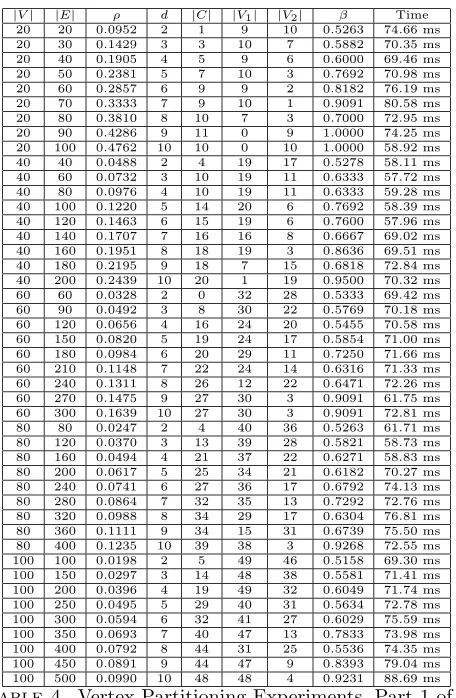
|V| |E| ρ d |C| |V1| |V2| β Time 20 20 0.0952 2 1 9 10 0.5263 74.66 ms 20 30 0.1429 3 3 10 7 0.5882 70.35 ms 20 40 0.1905 4 5 9 6 0.6000 69.46 ms 20 50 0.2381 5 7 10 3 0.7692 70.98 ms 20 60 0.2857 6 9 9 2 0.8182 76.19 ms 20 70 0.3333 7 9 10 1 0.9091 80.58 ms 20 80 0.3810 8 10 7 3 0.7000 72.95 ms 20 90 0.4286 9 11 0 9 1.0000 74.25 ms 20 100 0.4762 10 10 0 10 1.0000 58.92 ms 40 40 0.0488 2 4 19 17 0.5278 58.11 ms 40 60 0.0732 3 10 19 11 0.6333 57.72 ms 40 80 0.0976 4 10 19 11 0.6333 59.28 ms 40 100 0.1220 5 14 20 6 0.7692 58.39 ms 40 120 0.1463 6 15 19 6 0.7600 57.96 ms 40 140 0.1707 7 16 16 8 0.6667 69.02 ms 40 160 0.1951 8 18 19 3 0.8636 69.51 ms 40 180 0.2195 9 18 7 15 0.6818 72.84 ms 40 200 0.2439 10 20 1 19 0.9500 70.32 ms 60 60 0.0328 2 0 32 28 0.5333 69.42 ms 60 90 0.0492 3 8 30 22 0.5769 70.18 ms 60 120 0.0656 4 16 24 20 0.5455 70.58 ms 60 150 0.0820 5 19 24 17 0.5854 71.00 ms 60 180 0.0984 6 20 29 11 0.7250 71.66 ms 60 210 0.1148 7 22 24 14 0.6316 71.33 ms 60 240 0.1311 8 26 12 22 0.6471 72.26 ms 60 270 0.1475 9 27 30 3 0.9091 61.75 ms 60 300 0.1639 10 27 30 3 0.9091 72.81 ms 80 80 0.0247 2 4 40 36 0.5263 61.71 ms 80 120 0.0370 3 13 39 28 0.5821 58.73 ms 80 160 0.0494 4 21 37 22 0.6271 58.83 ms 80 200 0.0617 5 25 34 21 0.6182 70.27 ms 80 240 0.0741 6 27 36 17 0.6792 74.13 ms 80 280 0.0864 7 32 35 13 0.7292 72.76 ms 80 320 0.0988 8 34 29 17 0.6304 76.81 ms 80 360 0.1111 9 34 15 31 0.6739 75.50 ms 80 400 0.1235 10 39 38 3 0.9268 72.55 ms 100 100 0.0198 2 5 49 46 0.5158 69.30 ms 100 150 0.0297 3 14 48 38 0.5581 71.41 ms 100 200 0.0396 4 19 49 32 0.6049 71.74 ms 100 250 0.0495 5 29 40 31 0.5634 72.78 ms 100 300 0.0594 6 32 41 27 0.6029 75.59 ms 100 350 0.0693 7 40 47 13 0.7833 73.98 ms 100 400 0.0792 8 44 31 25 0.5536 74.35 ms 100 450 0.0891 9 44 47 9 0.8393 79.04 ms 100 500 0.0990 10 48 48 4 0.9231 88.69 ms
Table 4. Vertex Partitioning Experiments, Part 1 of 2
Robert H. Lewis
Department of Mathematics Fordham University
|V| |E| ρ d |C| |V1| |V2| β Time 120 120 0.0165 2 6 59 55 0.5175 70.06 ms 120 180 0.0248 3 21 59 40 0.5960 70.90 ms 120 240 0.0331 4 26 54 40 0.5745 72.52 ms 120 300 0.0413 5 36 54 30 0.6429 73.43 ms 120 360 0.0496 6 39 45 36 0.5556 63.93 ms 120 420 0.0579 7 50 47 23 0.6714 65.50 ms 120 480 0.0661 8 50 35 35 0.5000 65.07 ms 120 540 0.0744 9 52 31 37 0.5441 66.05 ms 120 600 0.0826 10 54 22 44 0.6667 66.48 ms 140 140 0.0142 2 8 69 63 0.5227 70.93 ms 140 210 0.0213 3 20 68 52 0.5667 73.76 ms 140 280 0.0284 4 33 66 41 0.6168 73.80 ms 140 350 0.0355 5 41 63 36 0.6364 78.15 ms 140 420 0.0426 6 47 60 33 0.6452 74.65 ms 140 490 0.0496 7 54 50 36 0.5814 79.88 ms 140 560 0.0567 8 59 67 14 0.8272 67.15 ms 140 630 0.0638 9 61 63 16 0.7975 66.69 ms 140 700 0.0709 10 65 57 18 0.7600 75.43 ms 160 160 0.0124 2 8 80 72 0.5263 71.23 ms 160 240 0.0186 3 25 79 56 0.5852 73.84 ms 160 320 0.0248 4 36 74 50 0.5968 75.24 ms 160 400 0.0311 5 43 66 51 0.5641 75.41 ms 160 480 0.0373 6 59 66 35 0.6535 77.78 ms 160 560 0.0435 7 61 67 32 0.6768 77.57 ms 160 640 0.0497 8 65 65 30 0.6842 71.26 ms 160 720 0.0559 9 72 46 42 0.5227 67.61 ms 160 800 0.0621 10 75 28 57 0.6706 76.35 ms 180 180 0.0110 2 6 89 85 0.5115 64.23 ms 180 270 0.0166 3 28 87 65 0.5724 65.60 ms 180 360 0.0221 4 34 85 61 0.5822 73.36 ms 180 450 0.0276 5 50 86 44 0.6615 64.37 ms 180 540 0.0331 6 65 84 31 0.7304 68.36 ms 180 630 0.0387 7 69 82 29 0.7387 68.46 ms 180 720 0.0442 8 79 87 14 0.8614 67.67 ms 180 810 0.0497 9 80 83 17 0.8300 71.01 ms 180 900 0.0552 10 84 88 8 0.9167 76.07 ms 200 200 0.0100 2 13 99 88 0.5294 61.56 ms 200 300 0.0149 3 30 99 71 0.5824 72.98 ms 200 400 0.0199 4 46 95 59 0.6169 74.56 ms 200 500 0.0249 5 54 85 61 0.5822 75.95 ms 200 600 0.0299 6 67 91 42 0.6842 69.84 ms 200 700 0.0348 7 73 72 55 0.5669 69.95 ms 200 800 0.0398 8 80 90 30 0.7500 73.63 ms 200 900 0.0448 9 86 48 66 0.5789 77.18 ms 200 1000 0.0498 10 93 96 11 0.8972 73.69 ms
n d true alpha prediction abs error rel error
25 2 0.51855 0.51039 -0.00816 -1.57%
25 3 0.55508 0.58648 0.03140 5.66%
25 4 0.60108 0.61405 0.01297 2.16%
25 5 0.63551 0.64142 0.00591 0.93%
25 6 0.68269 0.67683 -0.00586 -0.86%
25 7 0.72733 0.73054 0.00321 0.44%
25 8 0.80355 0.79510 -0.00845 -1.05%
25 9 0.87544 0.88098 0.00554 0.63%
25 10 0.93626 0.97436 0.03810 4.07%
50 2 0.51550 0.50869 -0.00681 -1.32%
50 3 0.56609 0.58003 0.01394 2.46%
50 4 0.60961 0.60380 -0.00581 -0.95%
50 5 0.63884 0.62197 -0.01687 -2.64%
50 6 0.66424 0.64762 -0.01662 -2.50%
50 7 0.71550 0.68465 -0.03086 -4.31%
50 8 0.76743 0.73365 -0.03378 -4.40%
50 8 0.76743 0.73365 -0.03378 -4.40%
50 9 0.82509 0.79405 -0.03104 -3.76%
50 9 0.82509 0.79405 -0.03104 -3.76%
50 10 0.87989 0.86495 -0.01494 -1.70% 50 10 0.87989 0.86495 -0.01494 -1.70%
75 2 0.51164 0.50804 -0.00360 -0.70%
75 3 0.55805 0.57864 0.02059 3.69%
75 4 0.59384 0.59993 0.00608 1.02%
75 5 0.62633 0.61530 -0.01103 -1.76%
75 6 0.64058 0.63656 -0.00401 -0.63%
75 7 0.66363 0.66868 0.00504 0.76%
75 8 0.69095 0.71040 0.01945 2.81%
75 9 0.77376 0.76328 -0.01048 -1.35%
75 10 0.81330 0.82356 0.01026 1.26%
100 2 0.51895 0.50769 -0.01126 -2.17% 100 2 0.51895 0.50769 -0.01126 -2.17%
100 3 0.56334 0.57719 0.01385 2.46%
100 3 0.56334 0.57719 0.01385 2.46%
100 4 0.59367 0.59783 0.00416 0.70%
100 4 0.59367 0.59783 0.00416 0.70%
100 5 0.62718 0.61134 -0.01583 -2.52% 100 5 0.62718 0.61134 -0.01583 -2.52% 100 6 0.64282 0.63059 -0.01223 -1.90% 100 6 0.64282 0.63059 -0.01223 -1.90% 100 7 0.66420 0.65928 -0.00492 -0.74% 100 7 0.66420 0.65928 -0.00492 -0.74%
100 8 0.69631 0.69783 0.00152 0.22%
100 8 0.69631 0.69783 0.00152 0.22%
100 9 0.75234 0.74548 -0.00686 -0.91% 100 9 0.75234 0.74548 -0.00686 -0.91% 100 10 0.82477 0.80118 -0.02359 -2.86% 100 10 0.82477 0.80118 -0.02359 -2.86% 125 2 0.51538 0.50747 -0.00791 -1.54%
125 3 0.56050 0.57682 0.01632 2.91%
125 4 0.59124 0.59650 0.00526 0.89%
125 5 0.61908 0.60908 -0.01000 -1.61% 125 6 0.63982 0.62679 -0.01302 -2.04% 125 7 0.65993 0.65388 -0.00605 -0.92%
125 8 0.66981 0.68985 0.02003 2.99%
125 9 0.68852 0.73505 0.04653 6.76%
125 10 0.77929 0.78697 0.00768 0.99%
150 2 0.51882 0.50732 -0.01151 -2.22% 150 2 0.51882 0.50732 -0.01151 -2.22%
150 3 0.56314 0.57612 0.01298 2.30%
150 3 0.56314 0.57612 0.01298 2.30%
150 4 0.59903 0.59557 -0.00345 -0.58% 150 4 0.59903 0.59557 -0.00345 -0.58% 150 5 0.62210 0.60732 -0.01478 -2.38% 150 5 0.62210 0.60732 -0.01478 -2.38% 150 6 0.63997 0.62415 -0.01583 -2.47% 150 6 0.63997 0.62415 -0.01583 -2.47% 150 7 0.65777 0.64969 -0.00808 -1.23% 150 7 0.65777 0.64969 -0.00808 -1.23%
150 8 0.67181 0.68428 0.01247 1.86%
150 8 0.67181 0.68428 0.01247 1.86%
150 9 0.71095 0.72711 0.01616 2.27%
150 9 0.71095 0.72711 0.01616 2.27%
150 10 0.79604 0.77706 -0.01899 -2.39% 150 10 0.79604 0.77706 -0.01899 -2.39%