SUPPORT VECTOR CHARACTERIZATION OF THE MICROSTRIP ANTENNAS BASED ON
MEASUREMENTS
N. T. Tokan and F. G¨une¸s
Department of Electronics and Communication Engineering Faculty of Electrics and Electronics
Yıldız Technical University Yıldız 34349, Istanbul, Turkey
Abstract—In this work, Support Vector Machine (SVM) formulation
is worked out based upon “L” measured data for the resonant
frequency, operation bandwidth, input impedance of a rectangular microstrip antenna. Results of the formulation are compared with the theoretical results obtained in literature, much better characterization is observed with greater accuracy. At the same time, Artificial Neural Network (ANN) is employed in generalization of the data on the resonant frequency, operation bandwidth, and input impedance of the antenna. Performances of the two advanced nonlinear learning machines are compared and superiority of the SVM is verified.
1. INTRODUCTION
Microstrip antennas have been used in aircraft, missile, satellite and many government and commercial applications, where size, weight, cost, performance, ease of installation and aerodynamic profile are constraints [1]. These antennas are low-profile, conformable to planar and non-planar surfaces, simple and inexpensive to manufacture using modern printed circuit technology, mechanically robust when mounted on rigid surfaces, compatible with MMIC designs, and when particular patch shape and mode selected they are very versatile in terms of resonant frequency, polarization, pattern and impedance [2].
(Fig. 1). Patch dimensions of rectangular microstrip antennas are usually designed so its pattern maximum is normal to the patch. Because of their narrow bandwidths and effectively operating in the vicinity of resonant frequency, the analysis of the microstrip antennas is very important.
Two kinds of theoretical approaches can be exploited in characterizing the resonant frequency, bandwidth, input impedance of the patch antennas. The first group starts from initial physical assumptions, which generally offers simple and analytical formulas, well suited for a physical understanding of phenomena and for future antenna computer-aided design (CAD). These methods are known as transmission-line models and cavity models. However, these methods do not consider rigorously the effects of surface waves. The second approach is based on an electromagnetic boundary problem, which leads to an expression as an integral equation, using proper Green functions, either in the spectral domain, or directly in the space
domain, using moment methods. Without any initial assumption,
the choice of test functions and the path integration appear to be more critical during the final, numerical solution. Exact mathematical formulations in the second group rigorous methods involve extensive numerical procedures, resulting in round-off errors, and may also need final experimental adjustments to the theoretical results. They are also time consuming and not easily included in a CAD system. However, the theoretical values obtained by using both these two theoretical methods are also not in very good agreement with the experimental results of both electrically thin and thick rectangular microstrip
antennas [3–5]. For these reasons, some numerical/experimental
methods for the analysis of microstrip antennas is worked out [6– 9]. In this work an advanced nonlinear learning machine, “Support Vector Machine (SVM)” is employed in analyzing the rectangular patch antenna, which enable to generalize ‘discrete’ data into the ‘continuous’ domain. In particular, SVMs are based on a judicious and rigorous mathematics combining the generalization and optimization theories together and verified to be computationally very efficient (the so-called Vapnik-Chervonenkis theory [10, 11]). This learning machine has found many fruitful applications in science and engineering, especially the typical applications in signal processing, modeling of microwave devices and antennas are given in [12–20].
In this work, SVMs are employed for regression in the analysis of the rectangular patch antennas, which in these types of applications, may be named as “Support Vector Regressors (SVR)”. Given a set of observed discrete data {(xi, yi) xi ∈Rn, yi ∈R, i= 1,2, . . . , L} the
approximation functionf(x) =b+yiαjK(xj,x) withy∼=f(x) for
regression andy= sgnf(x) for dichotomous classification for instance. In this work, data ensemble is provided from the experiments made in the literature. Thus, the three functions characterizing the antenna are approximated in terms of the geometrical parameters which include the electrical thickness, the dimensions of the rectangular patch, the parameter of the feeding position and the electrical properties of the used dielectric material. The outputs of the SVR functions for the patch antennas designed on the widely used dielectrics are compared with the target value, artificial neural networks (ANN) which are powerful tools in modeling of transmission lines and antennas [17–22] and the theoretical counterparts in the literature [3–5].
2. SUPPORT VECTOR MACHINES IN REGRESSION
The regression problem related to the estimation of the resonant frequency (fr), bandwidth (BW) and input impedance (Rin) functions
can be stated as follows: Firstly, let us consider fr. In the training
phase a set of L training pairs {(xo, fro), (x1, fr1), . . . ,(xL−1, frL−1)} is constructed by considering (x) as the input variable vector and (fr) as the output. Starting from these samples of the input/output
values of fr, the goal is to find a function ˜fr, which approximates as
well as possible unknown functionfr(x). By using the support vector
regression, ˜fr is defined as:
˜
fr(x) =w,ϕ(x)+b, (1)
where . . . denotes the inner product, ϕ is a nonlinear mapping vector that performs a transformation of the input vector to a
high-dimensional space. w and b are the weighting vector and bias,
respectively which are obtained by minimizing the primal convex objective function (Regression Risk), defined as [11]:
Rreg =
1
2w
2+C
L−1
i=0
Lε(x, fr,f˜r) (2)
where C is the regularization constant and Lε(x, f
r) is a general loss
function. Since the given objective function given in (2) has no
so-calledε-insensitive loss function developed by Vapnik [10] is used:
Lε(x, fr,f˜r) =
0, if fri−f˜r(xi)≤ε
fri−f˜r(xi)−ε, else
(3)
this defines anεtube so that if the predicted value is within the tube, the loss is zero, while if the predicted point is outside the tube, the loss is the magnitude of the difference between the predicted value and the radius of the tube.
According to [10] and [11], it is possible to recast the minimization of the regression risk as a dual optimization problem, in which the vector can be written in terms of the input dataxas:
w=
L−1
i=0
(αi−αi)ϕ(xi) (4)
where αi and αi are the unknown Lagrange multipliers. By
substituting (4) in (1), ˜Z0 is rewritten as ˜
fr(x) = L−1
i=0
(αi−αi)
φ(xi), φ(x) +b
=
L−1
i=0
(αi−αi)K(xi,x) +b (5)
and the coefficients αi, αi and must be chosen in order to minimize
the regression risk in the dual problem. In (5), the kernel function
K(xi,x) =φ(xi), φ(x)works on the original space. Commonly used kernels are polynomial and radial kernels.
Applying the standard Lagrange multiplier technique results in the equivalent maximization of the dual space objective function [11]:
W(α, α) = −ε
L−1
i=0
(αi+αi) + L−1
i=0
fri(αi−αi)
−1
2
L−1
i=0
(αi−αi)(αi +αi)K(xi,x) (6)
with the constraints:
0≤αi, αi≤C (7a)
L−1
i=0
The dual variablesαi, αi and bare computed using the
Karush-Kuhn-Tucker conditions [11] to maximize (6) subject to the constraints given by (7a), (7b). From Karush-Kuhn-Tucker conditions, it follows that only for|f˜r(xi)−fri| ≥ε, the Lagrange multipliers may be nonzero, or
in the other words for all samples inside theε-tube⇔ |f˜r(xi)−fri|< ε
the αi, αi vanish. Therefore we have a sparse expansion of w in
terms of xi (i.e., we do not need all xi to describe). The samples that come with nonvanishing coefficients are called Support Vectors. The idea of representing the solution by means of a small subset of
training points has also enormous computational advantages. This
reduced number of non-zero parameters together with the guaranteed global minimum gains superiority to support vector machines over the alternative methods. A detailed mathematical background together with the literature can be found in [11].
The regularization parameter C has been found to represent a measure of the tradeoff between the capabilities of the approach in estimating the resonant frequency of the patch antenna using training and test sets.
In order to correctly estimate the fr, L data pairs in the form:
{(xo, fo
r), (x1, fr1), . . . ,(xL−1, frL−1)} obtained from experimental
results for the rectangular patch antenna are used in the training phase. At the end of the training phase, in the so-called test phase for the new dielectric substrates and geometries not included in the training set,
fr is estimated. Similarly, support vector regressors can be applied to
the regression of the BW and Rin of the patch antenna. Numerical
details of the support vector regression analysis of the patch antennas will be given in the next section.
3. CHARACTERIZATION OF THE RECTANGULAR MICROSTRIP ANTENNA
3.1. Rectangular Microstrip Antennas
The rectangular microstrip antennas are made of a rectangular patch with dimensions, width, W, and length, L, over a ground plane with a substrate thickness, h and dielectric constant, εr, as given in Fig. 1.
Dielectric constants are usually used in the range of 2.2 ≤ εr ≤ 12.
Figure 1. Rectangular microstrip antenna.
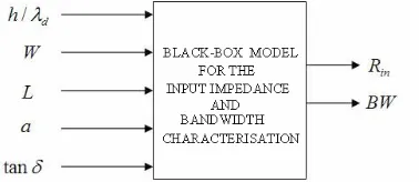
3.2. Black-Box Models for the Resonant Frequency, Bandwidth and Input Impedance
The black-box model is given in Fig. 2 for the training process of SVR and/or ANN characterization of bandwidth and input impedance. 27 data pairs of the experimental results in the literature [28–31] are exploited in the training process, while 6 data pairs are used
for the testing as shown in Tables 1–2. Thus, SVR is employed
in order to characterize the input impedance and bandwidth of the rectangular patch antenna as the functions of the antenna parameters of h/λd,W,L, a,tanδ with these measurement results. Here,h is the
thickness of the dielectric substrate, λd is the wavelength within the
substrate, W is the width of the patch, L is the length of the patch,
Table 1. The accuracies of the Rin, BW and fr functions in testing
process.
% accuracy SVR ANN
Rin 99.8 98.87
BW 97.85 98.81
fr 98.79 98.33
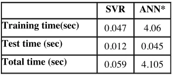
Table 2. Time analysis of ANN and SVR models for fr function of
the patch antenna.
SVR ANN*
Training time(sec) 0.047 4.06
Test time (sec) 0.012 0.045
Total time (sec) 0.059 4.105
(*trained for 300 epochs)
ais the position of the feeding point and tanδ is the loss tangent. Similarly, 37 and 9experimental data pairs [32–35] are used in the training and testing for the resonant frequency, respectively and its black-box model is given in Fig. 3. In this model, the resonant frequency of the rectangular patch antenna is obtained as the function of input variables ofW,L,h, εr. Here, εr is the dielectric constant of
the substrate. The input data of both models are normalized in the range of 0 and 1.
3.3. Generating of Support Vector Regression/Artificial Neural Network for the Characterization of Microstrip Antennas
In SVR, radial basis function kernel is chosen as the most suitable kernel function in our application:
K(x,x) = exp
−γx−xi2
(8)
where the width parameterγis set to 0.1 for the optimum performance. Similarly, the regularization parameter, C is set to 1. 24 support vectors corresponding to the diameter (⇔ ε= 0.1) of the insensitive tube are found to be sufficient out of the 27 data pairs in the training of SVR model for the determination of Rin function. Similarly, 22
support vectors out of 27 data and 31 support vectors out of 37 data are used in the training of SVR models for the determination ofBW
and fr functions, respectively.
The performance of the SVR is compared with ANN, which is the most competitive technique to SVR. Thus, two multilayer perception (MLP) models are used for the modeling inside the two black-boxes given in Figs. 2 and 3. ANN model for Rin and BW characterization
has 5 and 4 neurons in its two hidden layers, and 2 output neurons. ANN model to characterize fr has 4 and 3 neurons in its two hidden
layers and a single output neuron. Hyperbolic tangent sigmoid and linear transfer functions were used in the hidden and output neurons, respectively for the MLP training.
3.4. Results of the SVR and/or ANN Characterization
The accuracies of the SVR and ANN models for the resonant frequency, bandwidth and input impedance are given in Table 1. One of the most important superiority of SVR to the ANN is much faster convergence rate with the sparse solution technique as seen from Table 2 where the computation efficiency of the SVR and ANN for regression of the fr
function is compared.
The test results of the SVR regression for theRin, BW and fr of
the rectangular patch antenna take place in Tables 3–5 comparatively with measured (target) values, ANN results and other theoretical values in the literature.
Table 3. Comparison of the SVR results for the input impedance with the target values, ANN results and theoretical results.
d
h/λ W L
a
tan Rinme RinSVR RinANN Rin[20] Rin[31] Rin[32]0.0384 18.1 19.6 6.27 0.001 58 58.09 57.24 36.2 83.7 63.2
0.066 13.37 14.12 4.75 0.002 52 51.89 51.48 36.9 67.9 57.4
0.1292 13.75 15.8 5.82 0.002 44 43.90 43.31 51.5 47.4 49
0.1475 10 15.2 3.45 0.002 45 45.10 44.49 46.4 310.1 228.3
0.1814 12.56 27.56 3.2 0.002 46 46.09 46.56 45 1041.6 508
0.2182 10.3 33.8 3.6 0.002 47 47.09 46.76 46.5 2488.8 785.9 δ
Table 4. Comparison of the SVR results for the bandwidth with the target values, ANN results and theoretical results.
d
h / W L
a
tanδ BWme BWSVR BWANN BW[28] BW[37] BW[38]0.0384 18.1 19.6 6.27 0.001 4.9 4.99 4.73 6.17 3.96 2.2
0.066 13.37 14.12 4.75 0.002 7.7 7.79 7.66 9.16 7.29 4.2
0.1292 13.75 15.8 5.82 0.002 15.9 14.93 15.83 15.11 18.06 10.5
0.1475 10 15.2 3.45 0.002 18 17.68 17.83 17.47 14.08 11.8
0.1814 12.56 27.56 3.2 0.002 20 19.89 19.85 19.66 10.10 14.54
0.2182 10.3 33.8 3.6 0.002 21.6 21.91 21.16 21.73 7.11 16.95 λ
Table 5. Comparison of the SVR results for the resonant frequency with the target values, ANN results and theoretical results.
W L h
ε
r fr me fr SVR fr ANN fr [2] fr [32] fr [39] fr [40] fr [41]1.81 1.96 0.157 2.33 4805 4829 4782 4824 4749 5014 4635 4520
1.337 1.412 0.2 2.55 6200 6209 6218 6201 6053 6653 5845 5682
1.375 1.580 0.476 2.55 5100 5143 4923 5092 4993 5945 4667 4407
1 1.52 0.476 2.55 5820 5840 5889 5352 5423 6180 4855 4576
1.256 2.756 0.952 2.55 3580 3618 3765 2983 3115 3408 2668 2485
1.03 3.38 1.281 2.55 3200 3178 3169 2474 2623 2779 2183 1992
1.7 1.1 0.3175 2.33 6800 6628 6876 7405 6806 8933 6958 6467
6.858 4.14 0.152 2.5 2200 2266 2301 2241 2204 2292 2208 2158
4. CONCLUSION
In this work, a new methodology for characterization of microstrip
antennas is presented. To aim this, Support Vector Regression is
adopted to theL-measured data of the rectangular patch antenna and its performance is compared with the closest counterpart, Artificial Neural Network. Support Vector Regression is found to be superior to the Artificial Neural Network with respects of generalization ability, convergence rate and computational efficiency. Moreover, both regression results are compared to the those of the pioneer theoretical analyses and it can be concluded that the theory is still insufficient for complete characterization to take into account all the effects of the system. Thus, in these cases, rigorous methodologies to regress are needed. This work also verifies that Support Vector Regression is one of the most advisable methodologies to be employed.
ACKNOWLEDGMENT
This work was supported by the The Scientific and Technological Research Council of Turkey.
REFERENCES
1. Balanis, C. A., Antenna Theory, John Wiley & Sons, Inc., 1997.
2. Bahl, J. and P. Bhartia, Microstrip Antennas, Artech House,
Dedham, MA, 1980.
3. Sa˘gıro˘glu, S., K. G¨uney, and M. Erler, “Calculation of bandwidth for electrically thin and thick rectangular microstrip antennas with the use of multilayered perceptions,”Int. Journal of RF and
Microwave CAE, Vol. 9, 277–286, 1999.
4. G¨uney, K., M. Erler, and S. Sa˘gıro˘glu, “Artificial neural networks for the resonant resistance calculation of electrically thin and thick rectangular microstrip antennas,”Electromagnetics, Vol. 20, 387– 400, 2000.
5. Karabo˘ga, D., K. G¨uney, S. Sa˘gıro˘glu, and M. Erler, “Neural computation of resonant frequency of electrically thin and thick rectangular microstrip antennas,” IEE Proc. Microwaves,
Antennas Propagation, Vol. 146, No. 2, 155–159, 1999.
6. Li, L. and Y.-J. Xie, “Efficient algorithm for analyzing microstrip antennas using fast-multipole algorithm combined with fixed real-image simulated method,”Journal of Electromagnetic Waves and
7. Akdagli, A., “An empirical expression for the edge extension in calculating resonant frequency of rectangular microstrip antennas with thin and thick substrates,”Journal of Electromagnetic Waves
and Applications, Vol. 21, No. 9, 1247–1255, 2007.
8. Kumar, P., T. Chakravarty, S. Bhooshan, S. K. Khah, and A. De, “Numerical computation of resonant frequency of gap coupled circular microstrip antennas,” Journal of Electromagnetic Waves
and Applications, Vol. 21, No. 10, 1303–1311, 2007.
9. Yang, R., Y.-J. Xie, D. Li, J. Zhang, and J. Jiang, “Bandwidth enhancement of microstrip antennas with metamaterial bilayered substrates,”Journal of Electromagnetic Waves and Applications, Vol. 21, No. 15, 2321–2330, 2007.
10. Vapnik, V. N., Statistical Learning Theory, Wiley, New York, 1998.
11. Cristianini, N. and J. Shawe-Taylor, An introduction to support
vector machines (and other kernel-based learning methods),
Cambridge University Press, 2000.
12. Ganapathiraju, A., J. E. Hamaker, and J. Picone, “Applications of support vector machines to speech recognition,” IEEE Trans.
on Signal Processing, Vol. 52, No. 8, 2348–2356, 2004.
13. Rojo- ´Alvarez, J. L., G. Camps-Valls, M. Mart´ınez-Ram´on, E. Soria-Olivas, A. Navia-V´azquez, and A. R. Figueiras-Vidal, “Support vector machines framework for linear signal processing,”
Signal Processing, Vol. 85, No. 12 , 2316–2326, 2005.
14. Wu, Y. Q., Z. X. Tang, B. Zhang, and Y. H. Xu, “Permeability measurement of ferromagnetic materials in microwave frequency
range using support vector machine regression,” Progress In
Electromagnetics Research, PIER 70, 247–256, 2007.
15. Christodoulou, C., M. Martinez-Ramon, and C. Balanis,
Support Vector Machines for Antenna Array Processing and
Electromagnetics, Morgan & Claypool Publishers, 2006.
16. Pastorino, M. and A. Randazzo, “A smart antenna system for direction of arrival estimation based on a support vector
regression,” IEEE Transactions on Antennas and Propagation,
Vol. 53, No. 7, 2161–2168, 2005.
17. Zhao, Q. and J. Principe, “Automatic target recognition with support vector machines,”Neural Information Processing Systems
Workshop on Large Margin Classifiers, Denver USA, December
18. Xia, L., R. Xu, and B. Yan, “LTCC interconnect modeling
by support vector regression,” Progress In Electromagnetics
Research, PIER 69, 67–75, 2007.
19. G¨une¸s, F., N. T¨urker, and F. G¨urgen, “Signal-noise support vector model of a microwave transistor,” Int. Journal of RF and
Microwave CAE, Vol. 17, 404–415, 2007.
20. Xu, Y. H., Y. Guo, L. Xia, and Y. Q. Wu, “A support vector regression based nonlinear modeling method for Sic Mesfet,”
Progress In Electromagnetics Research Letters, Vol. 2, 103–114,
2008.
21. G¨uney, K., C. Yildiz, S. Kaya, and M. T¨urkmen, “Artificial neural networks for calculating the characteristic impedance of air-suspended trapezoidal and rectangular-shaped microshield lines,”
Journal of Electromagnetic Waves and Applications, Vol. 20,
No. 9, 1161–1174, 2006.
22. Yildiz, C. and M. T¨urkmen, “Quasi-static models based
on artificial neural neworks for calculating the characteristic parameters of multilayer cylindrical coplanar waveguide and strip line,”Progress In Electromagnetics Research B, Vol. 3, 1–22, 2008. 23. Mohamed, M. A., E. A. Soliman, and M. A. El-Gamal, “Optimiza-tion and characteriza“Optimiza-tion of electromagnetically coupled patch an-tennas using RBF neural networks,” Journal of Electromagnetic
Waves and Applications, Vol. 20, No. 8, 1101–1114, 2006.
24. Zainud-Deen, S. H., H. A. Malhat, K. H. Awadalla, and E. S. El-Hadad, “Direction of arrival and state of polarization estimation using radial basis function neural network (RBFNN),” Progress
In Electromagnetics Research B, Vol. 2, 137–150, 2008.
25. Yildiz, C., K. G¨uney, M. T¨urkmen, and S. Kaya, “Neural models for coplanar strip line synthesis,” Progress In Electromagnetics
Research, PIER 69, 127–144, 2007.
26. Ayestar´an, R. G. and F. Las-Heras, “Near field to far field
transformation using neural networks and source reconstruction,”
Journal of Electromagnetic Waves and Applications, Vol. 20,
No. 15, 2201–2213, 2006.
27. Pozar, D. M., “Microstrip antennas,”Proc.. IEEE, Vol. 80, No. 1, 79–81, 1992.
28. Kara, M., “A novel technique to calculate the bandwidth of rectangular microstrip antenna elements with thick substrates,”
29. Kara, M., “A simple technique for the calculation of bandwidth of rectangular microstrip antenna elements with various substrate thicknesses,”Microwave Opt. Technol. Lett., Vol. 12, 16–20, 1996. 30. Kara, M., “The calculation of the input resistance of rectangular microstrip antenna elements with various substrate thicknesses,”
Microwave Opt. Technol. Lett., Vol. 13, 137–142, 1996.
31. Kara, M., “An efficient technique for the computation of the input resistance of rectangular microstrip antenna elements with thick substrates,” Microwave Opt. Technol. Lett., Vol. 13, 363– 369, 1996.
32. Carver, K. R., “Practical analytical techniques for the microstrip
antenna,” Proceedings of Workshop on Printed Circuit Antenna
Technology, New Mexico State University, Las Cruces, Oct. 1979.
33. Chang, E., S. A. Long, and W. F. Richards, “An experimental in-vestigation of electrically thick rectangular microstrip antennas,”
IEEE Trans. Antennas Propagat., Vol. AP-34, No. 6, 767–772,
1986.
34. Kara, M., “The resonant frequency of rectangular microstrip antenna elements with various substrate thicknesses,” Microw.
Opt. Technol. Lett., Vol. 11, 55–59, 1996.
35. Kara, M., “Closed-form expressions for the resonant frequency of rectangular microstrip antenna elements with thick substrates,”
Microw. Opt. Technol. Lett., Vol. 12, 131–136, 1996.
36. G¨uney, K., “Radiation quality factor and resonant resistance of rectangular microstrip antennas,”Microwave Opt. Technol. Lett., Vol. 7, 427–430, 1994.
37. Carver, K. R. and J. W. Mink, “Microstrip antenna technology,”
IEEE Trans. Antennas Propagat., Vol. AP-29, 2–24, 1981.
38. G¨uney, K., “Bandwidth of a resonant rectangular microstrip
antenna,”Microwave Opt. Technol. Lett., Vol. 7, 521–524, 1994.
39. Howell, J. Q., “Microstrip antennas,” IEEE Trans. Antennas
Propagat., Vol. AP-23, 90–93, 1975.
40. Hammerstad, E. O., “Equations for microstrip circuits design,”
Proceedings of Fifth European Microwave Conference, 268–272,
Hamburg, Sept. 1975.
41. James, J. R., P. S. Hall, and C. Wood, Microstrip Antennas —