ABSTRACT
ANXI JIA. Stochastic Capacity at Freeway Bottlenecks with Application to Travel Time Prediction. (Under the direction of Dr. Nagui M. Rouphail and Dr. Billy M. Williams.)
The stochastic nature of freeway bottleneck breakdown and queue discharge are
investigated in this study through a comprehensive analysis of sensor data collected at
bottleneck sites in the San Francisco Bay Area, California and San Antonio, Texas. A new
procedure is proposed to define the stochastic variation of the onset of freeway breakdown
and of queue discharge capacity based on time indexed field data of speed-flow profiles. The
former is developed as a function of average vehicle time headways preceding observed
conditions where both speed is below and density is above locally defined congested flow
thresholds. Full year 15-minute data series were used in the demonstration and testing of the
procedure, yielding a high degree of statistical confidence in the resulting headway
distribution parameter estimates. The statistical analysis indicated that the probability
function of freeway bottleneck pre-breakdown flow rates follows a generalized logistic
distribution. In addition, a recursive queue discharge model is proposed for bottleneck flows
under congested (queued) conditions. The proposed queue discharge model is a simple
autocorrelated time series recursion that is seeded with the corresponding pre-breakdown
flow and dampens to the mean queue discharge rate. The proposed stochastic models are
robust and accurate and represent a significant improvement in the understanding and
modeling of freeway bottleneck flow.
Focusing on investigating underlying reason of stochastic capacity and queue
trajectory data by using the simplified car following model and demonstrates experimental
distributions of stochastic wave speed and jam density. Despite the limitations due to some
simplified assumptions, it is reasonable to conclude that the heterogeneity of kjam and w at the micro-level results from individual driving behavior, and the corresponding stochastic
capacity and queue discharge rate observed in the field data (marco-level) are also generated
by the heterogeneity between individual driving behaviors.
Furthermore, in order to recognize and capture the stochastic day-to-day travel time
evolution process, this study tries to apply several theoretical approaches to explicitly
account for the travel time variability caused by stochastic capacity and demonstrate the
travel time variability in an empirical study. Comparisons are made between the travel time
predictions from stochastic and deterministic (HCM level) capacity under the same demand
level. The results show to what extent the stochastic capacity contributes to the observed
Stochastic Capacity at Freeway Bottlenecks with Application to Travel Time Prediction
by Anxi Jia
A dissertation submitted to the Graduate Faculty of North Carolina State University
in partial fulfillment of the requirements for the Degree of
Doctor of Philosophy
Civil Engineering
Raleigh, North Carolina
2013
APPROVED BY:
--- Chair of Advisory Committee
Dr. Nagui M. Rouphail
--- --- Co-Chair Dr. Billy M. Williams Dr. Joseph Hummer
DEDICATION
This dissertation is dedicated to my ever-supportive parents, Feinan Zhao and
BIOGRAPHY
Anxi Jia was born on November 16th 1982 in the city of Taiyuan, China. He earned a Bachelor of Science degree in Computer Science and Technology in July, 2004, from Xidian
University, Xi’an, China. He obtained the Master of Science degree in Transportation
Engineering in August, 2008, from Texas A&M University-Kingsville. He entered the Civil
Engineering program at North Carolina State University in 2008 and expects to graduate with
a PH.D in May, 2013.
During his time at N.C. State, Anxi served as a graduate research assistant on several
research projects under advisor Dr. Nagui M. Rouphail and Dr. Billy M. Williams. After
ACKNOWLEDGMENTS
First and foremost, I would like to express my deepest gratitude to my advisor, Dr.
Nagui M. Rouphail, and my co-advisor, Dr. Billy M. Williams. Their guidance, passion for
the sharing of knowledge, and tireless dedication has been inspirational over the past four
years. Their advice, support and ideas make this research possible. It was personally a
rewarding experience to work with them.
I would also like to extend a special thank you to the committee members Dr. Joseph
Hummer, Dr. Xuesong Zhou and Dr. Peter Bloomfield. Dr. Hummer’s vision and broad
outlook helped this study throughout the process and his questions made it stronger. Dr.
Zhou’s ability to immediately absorb new ideas and share insight provides invaluable
resource to achieve my goals. Dr. Bloomfield’s expertise in the field of Statistics provides
invaluable guidance and technical support through this study.
I would also like to thank the entire C-05 research team, including Wayne Kittelson,
Brandon Nevers, William Reynolds, Hyejung Hu, and Li Jin. Their time and contributions
set the foundation for this study, and their ideas and feedback were invaluable.
Special thanks to Thomas Chase, Zachary Bugg, Sangkey Kim and Soheil Sajjadi for
the technique help.
TABLE OF CONTENTS
LIST OF TABLES ...viii
LIST OF FIGURES ... ix
1. INTRODUCTION ... 1
1.1 Background ... 1
1.2 Problem Statement ... 3
1.3 Research Objectives ... 7
1.4 Dissertation Organization ... 8
2. LITERATURE REVIEW ... 10
2.1 Stochastic Capacity Concept ... 10
2.2 State of the Practice of Breakdown Identification ... 11
2.3 Stochastic Capacity Models ... 13
2.4 Effects of Stochastic Capacity on Dynamic Traffic Assignment Models ... 15
2.4.1 Conceptual Framework ... 17
2.4.2 Route Choice Utility Function and Route Switching Rule ... 18
2.5 Impacts of Stochastic Capacity on Travel Time Prediction ... 22
3. STOCHASTIC CAPACITY MODELS AT MACRO-LEVEL ... 25
3.1 Data and Study Site Description ... 25
3.2 Breakdown Determination ... 31
3.3 Models for Stochastic Capacity and Queue Discharge ... 36
3.3.2 Stochastic Queue Discharge Model ... 45
3.4 Implementation of Stochastic Capacity Model into DTA Simulation Tool... 52
3.5 Summary ... 63
4. INVESTIGATING STOCHASTIC CAPACITY AT MICRO-LEVEL... 65
4.1 Data Description ... 65
4.2 Methodology ... 68
4.3 Stochastic Wave Speed and Jam Density ... 72
4.4 Correlation with the Deterministic Capacity at Marco-Level ... 81
4.5 Summary ... 83
5. INVESTIGATING TRAVEL TIME VARIABILITY WITH EMPRIRICAL STUDY ... 85
5.1 Study Site ... 86
5.2 Formulate Demand and Capacity distribution ... 89
5.2.1 Stochastic Capacity Distribution ... 89
5.2.2 Demand Distribution ... 90
5.3 Formulate travel time prediction function ... 98
5.3.1 BPR Function ... 99
5.3.2 Queuing Theory Approach ... 104
5.3.3 Shock Wave Theory ... 110
5.4 Summary ... 125
6. SUMMARY, CONCLUSIONNS AND RECOMMENDATIONS ... 127
6.2 Conclusion ... 129
6.3 Recommendations ... 130
7. REFERENCES ... 132
APPENDICES ... 140
APPENDIX A: CANDIDATE STUDY SITES ... 141
APPENDIX B: FLOW-SPEED CURVES OF STUDY SITES ... 145
APPENDIX C: GOODNESS OF FIT OF THE CAPACITIES... 148
APPENDIX D: THE DISTRIBUTIONS OF CAPACITIES ... 162
APPENDIX E: THE DISTRIBUTIONS OF DEMAND ... 166
LIST OF TABLES
Table 3.1 Information provided in Transguide database ... 26
Table 3.2 Information provided in Bay Area database ... 27
Table 3.3 Basic Information for the Study Sites ... 30
Table 3.4 Calibrated Traffic Parameters for Each Study Site ... 35
Table 3.5 Summary of Pre-breakdown Observations Screening Results ... 38
Table 3.6 Summary of Pre-breakdown Flow Rate Distribution Parameters ... 43
Table 3.7 Summary of Fitted Queue Discharge Model ... 48
Table 3.8 Statistics of the Duration of Breakdown ... 50
Table 3.9 Parameter Estimation of the Cumulative Logistic Regression ... 51
Table 3.10 Network-wide Travel Time Characteristics of Alternative Improvement Strategies ... 62
Table 5.1 Parameters of Demand Distribution for Different time Periods ... 93
Table 5.2 The RMSD of Average Travel Time ... 124
LIST OF FIGURES
Figure 1.1 Weekday Travel Times on SH-520 ... 2
Figure 2.1 I-880 Speed Flow Data ... 13
Figure 2.2 Estimated Capacity Distribution for Freeway A1 ... 14
Figure 3.1 Location of bottlenecks and Detectors in San Antonio Area ... 29
Figure 3.2 I-880 Speed Flow Data ... 32
Figure 3.3 Illustrations of the Identification of Pre-breakdown and Breakdown ... 36
Figure 3.4 Pre-breakdown Flows and Outliers for I-880 ... 40
Figure 3.5 Probability Density and Cumulative Distribution of Pre-Breakdown Flow Rate for I-880 ... 44
Figure 3.6 Simplified Recursive Queue Discharge Model ... 47
Figure 3.7 Portland Network Study Area ... 52
Figure 3.8 Network-Wide Simulation Results ... 59
Figure 3.9 Locations of OR-217 and TV Highway in the Network ... 60
Figure 4.1 Study Area for NGSIM US 101 Data (Source: (42)) ... 66
Figure 4.2 Study Area for NGSIM I-80 data (Source: (42)) ... 67
Figure 4.3 Vehicles’ Trajectories according to Newell’s Car Following Model ... 69
Figure 4.4 An Example of Stop-and-go Condition from NGSIM Data ... 70
Figure 4.5 Typical Triangular Flow-Density Diagram ... 71
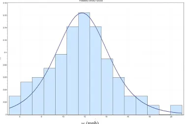
Figure 4.6 Distribution of w ... 72
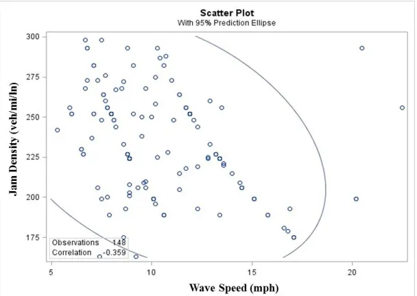
Figure 4.8 Scatter Plot of Jam Density and Wave Speed ... 76
Figure 4.9 The Distribution of Stochastic Capacity in Respond to the Distribution of kjam and w ... 78
Figure 4.10 The Distribution of Stochastic Capacity at Macro-level ... 79
Figure 4.11 The Distribution of Speed Observed at Capacities... 80
Figure 4.12 Wave Propagation along a Platoon... 81
Figure 5.1 Study Site... 86
Figure 5.2 Average Travel Time of the Target Link from Inrix ... 88
Figure 5.3 Travel Time Standard Deviation of the Target Link from Inrix ... 88
Figure 5.4 Stochastic Capacity Distribution of Target Link ... 89
Figure 5.5 Example of Traffic Demand Estimation ... 92
Figure 5.6 Demand Distribution for Time Period 6:00 – 6:15 ... 94
Figure 5.7 Correlation between Demands at Two Consecutive Time Intervals ... 94
Figure 5.8 Implementation Framework of Stochastic Capacity Generation ... 97
Figure 5.9 Average Travel Time: BPR Simulation vs. Inrix (Deterministic Capacity) ... 100
Figure 5.10 Travel Time Standard Deviation: BPR Simulation vs. Inrix (Deterministic Capacity) ... 101
Figure 5.11 Average Travel Time: BPR Simulation vs. Inrix (Stochastic Capacity) ... 102
Figure 5.13 Average Travel Time: Queuing Simulation vs. Inrix (Deterministic
Capacity) ... 106
Figure 5.14 Travel Time Standard Deviation: Queuing Simulation vs. Inrix (Deterministic Capacity) ... 107
Figure 5.15 Average Travel Time: Queuing Simulation vs. Inrix (Stochastic Capacity) .... 109
Figure 5.16 Travel Time Standard Deviation: Queuing Simulation vs. Inrix (Stochastic Capacity) ... 110
Figure 5.17 Illustrative Example of Wave Propagation with Stochastic Demand and Capacity ... 111
Figure 5.18 Demonstration of Wave Propagation for the Illustrative Example ... 113
Figure 5.19 Summary of Shock Wave Propagation ... 114
Figure 5.20 Illustrative Example of Vehicle Delay Calculation ... 117
Figure 5.21 Average Travel Time: Shockwave Simulation vs. Inrix (Deterministic Capacity) ... 120
Figure 5.22 Travel Time Standard Deviation: Shockwave Simulation vs. Inrix (Deterministic Capacity) ... 121
Figure 5.23 Average Travel Time: Shockwave Simulation vs. Inrix (Stochastic Capacity)122 Figure 5.24 Travel Time Standard Deviation: Shockwave Simulation vs. Inrix (Stochastic Capacity) ... 123
Figure F-1 Comprehensive Conceptual Simulation Framework ... 170
1. INTRODUCTION 1.1 Background
Traffic congestion problems lead to a wide range of adverse consequences such as
traffic delays, travel time unreliability, increased noise pollution, as well as air quality
deterioration. Broadly speaking, traffic congestion occurs because the available capacity
cannot serve the desired demand on a portion of roadway at a particular time. Major sources
of congestion include physical bottlenecks, incidents, work zones, bad weather, poor signal
timing, special events and day-to-day fluctuations in normal traffic (1). Among the seven major congestion sources, physical system bottlenecks, the primary source of recurring
congestion, contribute 40% of the travel delay on roadway networks (1), which is much greater than the others. Therefore, considerable research efforts have been devoted to
understanding the impacts of these physical bottlenecks and analyzing the effectiveness of
different traffic mitigation strategies.
To address the impacts of physical bottlenecks, capacity enhancement strategies,
including both construction and operational strategies, were widely studied by transportation
agencies. A challenge to both transportation practitioners and decision makers is quantifying
the effects of these capacity enhancement strategies for the purposes of making investment
decisions. Data from field measurement are costly and not readily available to support
decision-making. Moreover, their benefits may vary by local conditions, such as
transportation network complexity, traffic demand, driver behavior, etc. Therefore, traffic
study congestion caused by physical bottlenecks and analyze the effectiveness of various
capacity enhancement strategies.
Day-to-day/within-day variations in travel conditions pose a big challenge in a
simulation study. For example, Figure 1.1 shows the weekday travel time patternsfrom 5:00
PM to 6:00 PM on State Highway (SH) 520 Eastbound, Seattle, WA (1).
(Source: http://onlinepubs.trb.org/onlinepubs/webinars/PredictingTravelTimeReliabilityPresentations.pdf) Figure 1.1 Weekday Travel Times on SH-520
Based on the travel time pattern, there are obvious travel time variations on this route
even on normal weekdays (i.e., no incidents and good weather). Conventionally, it is widely
believed that the day-to-day demand variations result in a fluctuation of the travel time
pattern. This conclusion is made based on the assumption that the road capacity is always
Strategic Highway Research Program (SHRP2), titled "Understanding the Contribution of
Operations, Technology, and Design to Meeting Highway Capacity Needs," was carried out
to investigate this issue. One primary finding from this project is the existence of variations
in roadway capacity at the physical bottlenecks in the transportation network. Therefore,
besides demand variability, it is quite possible that the capacity variance may also contribute
to the observed travel time fluctuation, because the travel time is the function of both demand
and capacity.
1.2 Problem Statement
There have been multiple studies aimed at understanding the impacts of physical
bottlenecks and analyzing the effectiveness of different traffic mitigation strategies (e.g., road
capacity enhancement). Both macroscopic and microscopic models have limitations when it
comes to evaluating capacity enhancement strategies in large-scale transportation networks.
For example, macroscopic models represent traffic flow in terms of aggregate measures such
as flow rate, density, and speed over the modeled time period. Consequently, they are not
sensitive to some operational effects of strategies, such as Advanced Traveler Information
Systems (ATIS), because they do not consider the constituent individual vehicles and cannot
identify more severe traffic problems presented during smaller time intervals. Although they
can still handle such operational effects as percent of traffic diverting, they cannot do it in the
adaptive and dynamic way since it is assumed that in macroscopic models, all vehicles in the
network have the same characteristics. Microscopic models represent individual vehicles’
changing models, etc. Although micro models can provide a more realistic representation of
traffic conditions and examine certain complex traffic scenarios, when handling relatively
large real-world transportation network the calibration and validation of micro model can be
exceedingly time consuming, and the simulation may require an inordinate amount of
computational resources compared to their macro counterpart.
Mesoscopic models are at the intermediate level between micro and macro models.
Mesoscopic models represent individual vehicle motion based on macroscopic traffic
relationships (ex., speed-density function), but not their interactions (2). Since mesoscopic models keep recording the travel experience of each individual vehicle, they are normally
used as an evaluation tool for traveler information systems. Mesoscopic models integrated
with Dynamic Traffic Assignment (DTA) (3, 4) have become popular tools for traffic analysts to perform such applications (i.e., capacity enhancement strategy assessment) on
large-scale transportation networks because of thier ability to allocate individual vehicle
within the network to their destination based on factors that affect their route choice. Over
the last three decades, the focus of DTA research has been on the demand characterization
side, such as incorporating dynamic time-dependent demand, stochastic departure times, and
multiple user classes.
By contrast, the supply side, in which link capacity is a critical factor that may
determine the impacts of physical bottlenecks and then the route choice, was mostly
overlooked by researchers in the field of DTA. Conventional static and dynamic traffic
examination of freeway detector data reveals that breakdowns occur across a wide range of
volumes. Even under constant geometric and operational conditions, road capacities vary
with time over a certain range around a mean value. Based on the capacity distribution
function derived from field data (refer to the data discussed in Chapter 3), the mean value of
capacity is about 1900 pc/h/ln, and the maximum capacity is about 2,370 pc/h/ln, which is
very close to the value predicted by Highway Capacity Manual (HCM) 2000.
Only recently has the research community begun to accept and study the stochastic
capacity concept. Similar to the traditional definition of capacity in the HCM, the queue
discharge flow rate is also typically characterized in a deterministic manner. In other words,
after a breakdown occurs, the queue will discharge at a constant flow rate. If the capacity
were stochastic, it also quite possible that after a breakdown occurs, the queue discharge rate
would be stochastic as well. However, few studies have investigated the characteristics of the
queue discharge at freeway bottlenecks. Therefore, the characteristics of the queue discharge
are also of interest in this study. It is expected that stochastic capacity/queue discharge
variability will significantly alter our traditional understanding of the physical bottlenecks
under breakdown and queue discharge conditions. Based on the discussion above, HCM
capacity levels are more representative of the upper tail of capacity distribution function
derived from the field data, and the expected or mean value of capacity appears to be
approximately 500 pc/h/ln lower than the HCM-based values. Correspondingly, conventional
network modeling tools, which rely on the HCM capacity levels, need to be improved by
frequency, duration, and, consequently, the traffic operational impact of network bottlenecks
as well as the impact of operational enhancements.
Roadway capacity has conventionally been a constant value. The implication of this
definition is that traffic breakdown will occur only if the traffic demand is greater than the
constant capacity, which is widely used in traffic condition analysis. However, this is not
consistent with field observations: examination of freeway detector data reveals that
breakdowns occur across a wide range of traffic volumes. As suggested by field data,
capacity could be better represented as a stochastic variable rather than a constant. As a
consequence, the stochastic capacity concept will significantly change the way that we
analyze traffic networks. For example, considering a single freeway bottleneck with certain
demand, the conventional deterministic capacity concept may suggest that breakdown will
never occur under this demand level (if the demand is less than the deterministic capacity
value) at this bottleneck, while in the stochastic capacity environment, the breakdown may
occur with certain probability, which depends on the demand level. Although stochastic
capacities have been observed and discussed by several researchers, there are not stochastic
capacity models readily available for real-world application. Therefore, continued research
is needed to increase understanding and provide realistic, implementable stochastic capacity
models for the physical bottlenecks.
As discussed above, the stochastic capacity concept will significantly change the way
that we look at the traffic network. Therefore, some research hypothesis include: how can
measures, such as travel time or travel time variability? For example, observations in Figure
1.1, would seek to explore the extent to which the stochastic capacity contribute to the
observed travel time variability. Does the stochastic capacity really play an important role in
the travel time estimation? Furthermore, in the DTA simulation environment, travel time is
the key criterion for route switching in traffic assignment models. How will the travel time
variance introduced by stochastic capacity impact the traffic assignment models? Therefore,
a theoretical approach is needed to account for the travel time variability due to stochastic
capacity. This is a critical intermediate step to incorporate stochastic capacity into DTA
simulation tools.
1.3 Research Objectives
The objective of this study is to analyze stochastic characteristics of road capacity for
freeway physical bottlenecks and develop a theoretical approach to account for the travel
time variance introduced by stochastic capacity. More specific, this study will try to answer
following questions:
Does the stochastic capacity exist?
How to quantify the stochastic capacity and the corresponding queue
discharge?
What is the possible underlying reason of the stochastic characteristics?
Is stochastic capacity important for the traffic analysis (ex., travel time
This research is expected to produce a better understanding of stochastic capacity and
queue discharge for freeway bottlenecks and a realistic assessment of its impacts in the
transportation network. It is expected to improve the capability of analytical or simulation
models in terms of addressing travel time variation caused by stochastic capacity and then
produce better estimations from these models for the travel time studies. It is also expected
that the results of this study will contribute to a more valid benefit/cost analysis of capacity
enhancement strategies so as to support the decision making by transportation planners.
1.4 Dissertation Organization
This dissertation is organized in six chapters:
Chapter 1 introduces background, problem statement, and objectives.
Chapter 2 presents a literature review of stochastic capacity concept, state of the
practice of breakdown identification, stochastic capacity models and the effects of stochastic
capacity on dynamic traffic assignment models.
Chapter 3 describes the analysis of stochastic capacity models at macro level,
including data description, study site selection, breakdown determination, stochastic capacity
model for freeway bottlenecks, stochastic queue discharge model and the implementation of
stochastic capacity model into DTA simulation tool.
Chapter 4 presents the analysis of stochastic capacity at micro level with the focus on
Chapter 5 presents the importance of stochastic capacity and queue discharge concept
in traffic operational analysis by demonstrating to what extent the stochastic capacity can
contribute to the observed travel time variability.
2. LITERATURE REVIEW
In this chapter, studies on stochastic capacity as well as the state of the practice of
DTA models are reviewed.
2.1 Stochastic Capacity Concept
In the 2000 edition of the Highway Capacity Manual (HCM 2000), freeway capacity is defined as “the maximum hourly rate at which vehicles reasonably can be expected to
traverse a point or a uniform section of a roadway during a given time period under
prevailing roadway, traffic, and control conditions” (5). In keeping with this definition of
freeway capacity, it is widely accepted by most traffic analysts that the facility will
experience breakdown (i.e. a transition from an uncongested state to a congested state) only
if the traffic demand exceeds a specified capacity value. In other words, the breakdown is
treated as a deterministic phenomenon, and the freeway capacity is taken to be a constant
value. However, an emerging body of research (6-11) indicates that the traffic flow rate during the time intervals preceding observed instances of freeway breakdown (called
pre-breakdown flow rate in this study) is better represented as a random variable than a fixed
value. For example, Lorenz and Elefteriadou (10) clearly described the stochastic freeway capacity concept. The findings described in their paper indicate that breakdown is not a
deterministic event and that it could occur at any given flow rate with a finite probability
(zero probability at many low flow rates). This suggests that breakdown could occur across a
wide range of volumes and the probability of the breakdown occurrence varies by the
nature of freeway capacity, Lorenz and Elefteriadou (10) also suggested a new terminology, called sustainable flow rate, as the substituent of conventional deterministic capacity. The
sustainable flow rate could be defined as the maximum flow rate up to which tolerable traffic
performance (i.e. certain breakdown probability) of the facility is achieved and beyond which
intolerable traffic conditions are likely to arise. As the tolerable traffic performance is
defined differently, the sustainable flow rate may vary correspondingly even for a same
roadway segment, which makes the sustainable flow rate a stochastic variable in contrast to
the conventional deterministic capacity. Although these studies did not quantify the capacity
variations, they do demonstrate the stochastic nature of freeway capacity through the analysis
of real-world traffic data.
2.2 State of the Practice of Breakdown Identification
Breakdown determination is the critical starting point for both stochastic capacity and
queue discharge studies. In current practice, the flow rates just preceding the breakdown
condition are used to analyze the freeway stochastic capacity. The flow rate data are typically
time indexed data aggregated at five- or fifteen-minute intervals. The studies specified a
critical speed or a critical speed drop to define the freeway breakdown. However, while such
a speed‐based threshold can be well defined in reference to representative traffic flow
characteristics, the threshold value will vary by location. For example, extensive analysis of
Los Angeles freeway data suggests that free flow speed is around 60 mph and that at
to identify a breakdown event using five‐minute data. Using data obtained from Toronto
freeways, on the other hand, Elefteriadou defined that breakdown occurred “when the
average speed of all lanes on the freeway dropped below 90 km/hr (56mph) for a period of at
least five minutes” (13). These examples clearly illustrate that setting a specific, universal
speed threshold is not advisable and the threshold for breakdown identification requires local
calibration. Instead freeway breakdown analyses should be based upon speed thresholds
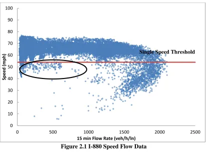
extracted from the speed flow observations. Moreover, a recent study by Jia et al. (14) suggests that it is problematic to use speed as the only criterion to define breakdown. Based
on the 15-minute sensor data from I-880 in the San Francisco Bay Area (Figure 2.1), they
found that a single speed threshold was not considered sufficient for determining congested
conditions. As shown in Figure 2.1, by applying a single speed threshold (speed differential
of 20 mph), observed conditions exhibiting a flow rate lower than 1000 vph per lane but with
speeds higher than 40 mph were considered to be reflective of anomalous free‐flow
conditions rather than congested conditions. The presence of low flow observations below
the single speed threshold creates the need for a robust phase boundary for defining
Figure 2.1 I-880 Speed Flow Data
2.3 Stochastic Capacity Models
Zurlinden (15) and Brilon (16) developed a methodology to derive roadway pre-breakdown distribution functions for the purpose of implementing the stochastic capacity
concept. In the most recent study, Brilon (17) suggested the Weibull distribution for characterizing the stochastic capacity based on traffic data from German freeways. Based on
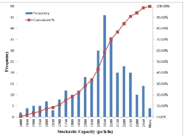
the probabilistic nature of freeway capacity, Dong and Mahmassani (18) first illustrated the significant effects of the stochastic concept on travel time reliability. Figure 2.2 illustrates the
estimated stochastic capacity distribution for Freeway A1, a two-lane freeway segment in
Germany, developed in Brilon's study (17). 0 10 20 30 40 50 60 70 80 90 100
0 500 1000 1500 2000 2500
Sp e e d ( m p h )
15 min Flow Rate (veh/h/ln)
(Source:
http://www.ruhr-uni-bochum.de/verkehrswesen/vk/deutsch/Mitarbeiter/Brilon/ISTTT16_Brilon_Geistefeldt_Regler_final_citation.pdf) Figure 2.2 Estimated Capacity Distribution for Freeway A1
As shown in the figure, a single capacity value is not appropriate for defining
breakdown on freeway bottlenecks. The trend illustrated by the figure also indicates that the
slope of the cumulative density function continually increase with increasing values of flow
rate. This trend is consistent with findings from previous studies (10, 17), which show the probability of breakdown increasing with increasing flow rate. Therefore, the freeway data
calibration results indicate that the HCM capacity levels are more representative of the upper
tail of the capacity observations and conversely are not representative of the expected or
Similar to the traditional definition of capacity in the HCM, the queue discharge flow
rate is also typically characterized in a deterministic manner. In other words, after a
breakdown occurs, the queue will discharge at a constant flow rate. Based on field data,
Lorenz and Elefteriadou (10) have clearly demonstrated that the queue discharge flow rate is also stochastic in nature. Further, Dong and Mahmassani (19) suggested a linear relationship between queue discharge rate and the pre-breakdown flow rate. In a most recent study, Jia
et.al, (14) concluded that the queue discharge rate series are strongly time-correlated and developed a recursive queue discharge model. In their model, the queue discharge rates
converge to the mean discharge rate for breakdowns that are initiated with stochastic average
pre-breakdown headway probability distribution.
2.4 Effects of Stochastic Capacity on Dynamic Traffic Assignment Models
As stated previously, conventional traffic assignment methods assume static,
deterministic segment capacity. Therefore, travel time on a path only depends on the flow
pattern on that path. In other words, for a fixed network-wide path flow pattern, the
corresponding path travel times do not change. Within the stochastic capacity concept,
however, real-world road capacities vary with time over a certain range, and a driver’s travel
experience on a single day can be dramatically affected by the underlying realized capacity
values on that particular day. In other words, travelers will experience different travel times
on the same path over different days even under the same path flow pattern because of the
inherent travel time variability introduced by stochastic capacity. As a result, conventional
method of successive averaging (MSA (20)), may not enable drivers to recognize and appropriately respond to the travel time variability/unreliability resulting from capacity
fluctuation. A theoretically rigorous and practically useful traveler route choice model is
crucially needed in order to adaptively capture the stochastic day-to-day travel time evolution
process and also to maintain robustness under disruptions due to stochastic capacity
reductions.
To better describe adaptive traveler behavior and simulate the resulting travel flow
pattern in an environment where roadway capacity varies within single day and over multiple
days, a day-to-day learning framework is needed to allow a realistic consideration and
evaluation of different capacity-enhancing and traffic management scenarios. A wide variety
of day-to-day learning models have been proposed to understand and simulate the
medium-term traffic evolution process under various advanced traveler information provision
strategies. An early study by Hu and Mahmassani (21) took into account both route and departure time choices as the sources of day-to-day traffic dynamics. Srinivasan and Guo
(22) examined network evolution (i.e., the network traffic condition or performance) and user response characteristics under varying market penetration levels of traveler information. Jha
et al. (23) adapted a Bayesian framework to model the traveler perception updating process. Chen and Mahmassani (24) further studied triggering mechanism and termination conditions for the travel time learning process. All existing day-to-day learning frameworks assume a
constant road capacity, and the variability sources considered in those models are limited to
road capacities vary with time over a certain range. In order to represent the traffic network
in a more realistic way, capacity variance should be incorporated with other variability
source. Correspondingly, the simulation frameworks should be improved to account for the
new variance introduced by stochastic capacity.
2.4.1 Conceptual Framework
The day-to-day learning framework proposed by Hu and Mahmassani (21) and Jha et al. (23), as shown in equation 2-1, 2-2 and 2-3, provides a promising path for seamlessly integrating stochastic capacity models in the DTA simulator for large-scale networks.
Generally speaking, the learning behavior in such a day-to-day learning framework is
determined by each vehicle’s historical travel experiences, the traveler information obtained
before and during the trip, as well as newly experienced travel times on the current day.
Conceptually, the model includes three components:
Traffic flow assignment model: (2-1)
Stochastic traffic system simulation process: (2-2)
Travel time perception model: (2-3)
Where:
= assigned route flow pattern on day d, determined by traffic assignment model/function
A(·),
= true travel time on day d, determined by dynamic assignment/simulation function S(·), = the system noise introduced by the stochastic capacity,
= the traveler perception error associated with perceived travel time in the network,
introduced by sampling error associated with personal experience and quality of information.
It should be noted that most existing day-to-day learning models are implemented
assuming stable road capacity, and therefore no system noise, i.e. , so the travel time
is a deterministic vector for a given set of route flows, in Equation 2-2. Accordingly,
the focus in previous research has been on how to reach the deterministic steady-state
conditions, and how to construct realistic learning/updating models for the travel time
perception error term related to Equation 2-3.
2.4.2 Route Choice Utility Function and Route Switching Rule
A behaviorally sound route choice utility function was proposed and calibrated by
Brownstone and Small (25) and Lam and Small (26), which considers the stochastic nature of traffic systems.
(2-4)
Where,
= generalized travel time (hour),
= the expected travel time for a traveler,
= perceived travel time variability.
= reliability ratio (computed as the ratio of Value of Reliability (VOR) and Value of Time
(VOT)).
TOLL = road toll charge; assumed to be zero in the following discussion as no toll-related
It has been well recognized that travel time variability and reliability are important
measures of service quality for travelers. In the above utility function, Equation 2-4, the
travel time standard deviation (TSD) is used to measure system travel time variability associated with the underlying stochastic traffic process. This contrasts with the perception
error variance in a deterministic assignment model. For a single traveler v, the route choice decision is made by comparing the generalized travel time of habitual path, , and that of
alternate path, . The traveler will switch to the alternative path from his/her habitual
path only if the following condition were met:
(2-5)
Where,
v = traveler index,
h=index for habitual path, and
a=index for potential alternative path.
According to Equation 2-4, if the generalized travel time of the habitual path, , is
greater than that of alternate path, , as shown in Equation 2-5, a driver should switch
his/her route from the habitual path to the alternative path. The resulting decision rule could
be derived as:
(2-6)
A bounded rationality model, which states that a driver’s decision depends on their
desired satisfaction level, is usually adapted to make the route choice comparison. The
from the early work by Mahmassani and Herman (27)) since Herbert Simon (28) pointed out that perfectly rational decisions are often not feasible given the limits of human cognition.
Based on the minimum acceptable absolute tolerance and the relative acceptable
tolerance, a set of bounded rationality rules, shown in Equation 2-7, are used to describe
users' route switching behavior. As opposed to the optimization theory in which users select
the best option from all possible decisions, in the bounded rationality approach, users perform limited searches, accepting the first satisfactory decision.
{ ̅
(2-7)
Where,
𝜹 =1, switch to an alternative path; 0, remain on the habitual/ current path,
α = Minimum acceptable absolute tolerance needed for a switch and ,
λ = Relative acceptable tolerance (i.e. relative improvement threshold).
However, by assuming constant demand level and stable road capacity (i.e., no
system noise, ), it is impossible to calculate the perceived travel time variability.
Therefore, in most studies, the above minimum acceptable absolute tolerance is always
assumed as a constant value in order to apply the bounded rationality approach. The models
proposed in the past to describe drivers' travel choice behavior are based on the assumption
that drivers select paths to minimize their perceived travel times (29).
As a result, most previous study efforts only focus on how to estimate the updated
averages of measured travel times on previous days. A simple extension of the above
approach would be to allow the weights to vary across individuals. Under the myopic
adjustment approach, Mahmassani and Chang (31) modeled drivers' travel choices based on the previous day's experience. The updating process is given by the following equation:
(2-8)
Where,
updated travel time by driver i;
experienced trip time by driver i on day d-1;
schedule delay of driver i on day d-1;
a, b = parameters reflecting the relative weights of earliness and lateness
binary variable such that for early arrival and otherwise ;
binary variable such that for late arrival and otherwise ;
Jhe et al. (23) proposed a perceived travel time updating model based on Bayesian updating. The perceived travel time is given by:
( ) (2-9)
Where,
prior mean;
Mean of the sample
parameter based on the updated variance.
Although it is not well known how the travel variability will impact the accuracy of
variability already constrains the analysis capability of the dynamic traffic assignment
simulation tools. For example, it is difficult to evaluate the travel variability, which has
become a very important operational criterion to assess the transportation network
performance.
Therefore, several studies have considered the stochastic demand in the simulation,
for example, by incorporating dynamic departure time choice. However, travel time is a
function of both demand and supply. It is also important to investigate whether the
incorporation of stochastic capacity will improve the estimation of travel time variability.
Within the stochastic capacity environment, it is reasonable to expect that drivers' perception
of travel time would change across different days.
2.5 Impacts of Stochastic Capacity on Travel Time Prediction
The researchers have realized that the incorporation of stochastic inputs (i.e., demand
and capacity) into the traffic system will significantly alter the characteristics of travel time,
especially the travel time variance. Focusing on analytical Bureau of Public Roads (BPR)
functions, which is widely used U.S., several studies have developed numerical
approximation methods to predict travel time variability distributions due to the stochastic
capacity or the stochastic demand. Lo and Tung (32) implemented the Mellin transforms-based method to estimate the mean and variance of travel time distribution due to the
stochastic capacity, which is modeled as a uniform probability distribution function. Through
a sensitivity analysis of the link representation in a network based on a multivariate normal
function of link travel times within stochastic demand environment. Ng and Waller (34) calculated the probability density function of travel time within stochastic capacity
environment by using a Fourier transformation approach. Recently, Zhou et al. (35) has derived the distribution of the link travel time based on BPR function. If demand, d, is assumed constant and the stochastic link capacity C follows a Lognormal distribution
( ), the link travel time can be estimated as:
( α ) (2-10)
Where,
link free-flow travel time
d = traffic demand
μc = mean of stochastic link capacity
σc = standard deviation of stochastic link capacity
α = coefficient of BPR function (often set at 0.15)
= exponent of BPR function (often set at 4.0)
Although several analytical studies have been conducted focusing on the BPR
function, it has been well known that the BPR function cannot effectively describe the
dynamic buildup and dissipation of traffic system congestion. Therefore, the travel time
estimation studies above based on BPR function are more suitable for analyzing long-term
steady-state traffic equilibrium results (35). A robust theoretical approach is required to account for the travel time variability introduced by stochastic capacity, especially under
and therefore the approach should incorporate both stochastic demand and capacity
simultaneously.
3. STOCHASTIC CAPACITY MODELS AT MACRO-LEVEL
In this chapter, the stochastic capacity models developed at Marco-level are
summarized. This chapter is organized as follows. Section 3.1 first introduces the field
dataset used to develop the stochastic capacity models. This is followed by the breakdown
identification procedure (section 3.2), and the stochastic capacity models in terms of
pre-breakdown flow and queue discharge (section 3.3).
3.1 Data and Study Site Description
In this study, data were assembled from the TransGuide system (36) in San Antonio,
Texas, and from PeMS data (37) archived for the San Francisco Bay Area (CALTRANS
District 4) in California. Data for both locations are available from online databases. The
TransGuide database provides traffic volume, speed, and occupancy data gathered from the
initial 26 miles of instrumented highways within the Texas Department of Transportation
TransGuide project. The extracted data set for this study is the daily raw data (20 sec.
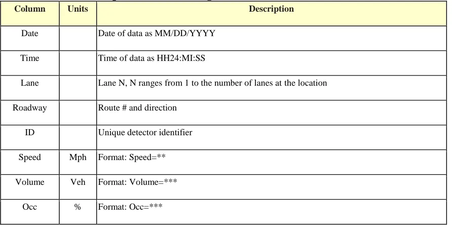
intervals) from 01/01/2007 to 09/30/2008. The information provided by TransGuide database
is summarized in the Table 3.1.
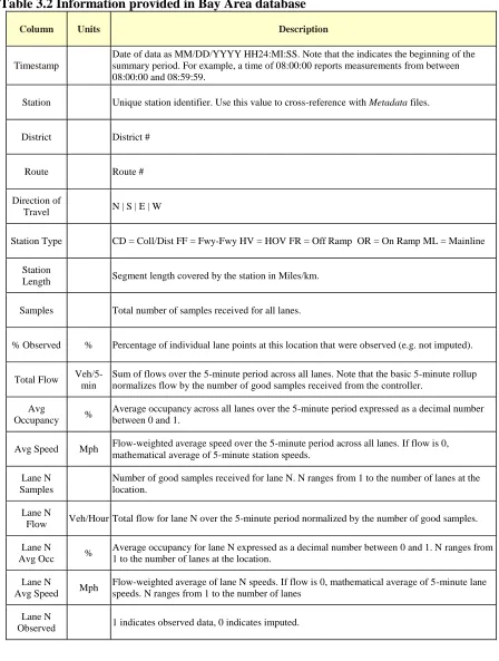
The Bay Area data used in this study are processed traffic data, which include volume,
speed, and occupancy. The data covered the period from 01/01/2007 to 09/30/2008
aggregated at a five-minute interval. The information provided by the PeMS database is
Table 3.1 Information provided in Transguide database
Column Units Description
Date Date of data as MM/DD/YYYY
Time Time of data as HH24:MI:SS
Lane Lane N, N ranges from 1 to the number of lanes at the location
Roadway Route # and direction
ID Unique detector identifier
Speed Mph Format: Speed=**
Volume Veh Format: Volume=***
Occ % Format: Occ=***
Since the Bay area data were pre-processed and aggregated by PeMS, there are no
missing observations in the dataset. For TransGuide data, however, there are a small number
of missing observations. Therefore, before performing the data aggregation, the
corresponding days with missing observations were removed from the dataset. Because the
entire dataset covers twenty-one months and the missing observations represented a small
portion of the data set, deletion of the missing values is a reasonable approach. Both
TransGuide and PeMS databases provide detailed location information for each sensor on the
freeway system. As discussed below, this detailed location data are important for selecting
Table 3.2 Information provided in Bay Area database
Column Units Description
Timestamp
Date of data as MM/DD/YYYY HH24:MI:SS. Note that the indicates the beginning of the summary period. For example, a time of 08:00:00 reports measurements from between 08:00:00 and 08:59:59.
Station Unique station identifier. Use this value to cross-reference with Metadata files.
District District #
Route Route #
Direction of
Travel N | S | E | W
Station Type CD = Coll/Dist FF = Fwy-Fwy HV = HOV FR = Off Ramp OR = On Ramp ML = Mainline
Station
Length Segment length covered by the station in Miles/km.
Samples Total number of samples received for all lanes.
% Observed % Percentage of individual lane points at this location that were observed (e.g. not imputed).
Total Flow Veh/5-min
Sum of flows over the 5-minute period across all lanes. Note that the basic 5-minute rollup normalizes flow by the number of good samples received from the controller.
Avg
Occupancy %
Average occupancy across all lanes over the 5-minute period expressed as a decimal number between 0 and 1.
Avg Speed Mph Flow-weighted average speed over the 5-minute period across all lanes. If flow is 0, mathematical average of 5-minute station speeds.
Lane N Samples
Number of good samples received for lane N. N ranges from 1 to the number of lanes at the location.
Lane N
Flow Veh/Hour Total flow for lane N over the 5-minute period normalized by the number of good samples.
Lane N
Avg Occ %
Average occupancy for lane N expressed as a decimal number between 0 and 1. N ranges from 1 to the number of lanes at the location.
Lane N
Avg Speed Mph
Flow-weighted average of lane N speeds. If flow is 0, mathematical average of 5-minute lane speeds. N ranges from 1 to the number of lanes
Lane N
As a basis for developing and demonstrating the stochastic freeway bottleneck
models, the most common freeway bottleneck feature, i.e. on-ramp junctions, was selected
for detailed study. The ideal bottlenecks for this study should be the on-ramp junctions with a
sufficient number of breakdown observations. PeMS system has listed the active bottlenecks
in Bay Area. The analyst selected the locations where congestion occurs more than during 10
or more days per month as the candidate study sites in Bay Area. Compared with PeMS
system, the TransGuide database did not indicate the active bottlenecks in the freeway
network. Therefore, what the analyst did firstly is to record all geometric bottlenecks through
Google Map in the areas covered by TransGuide detectors. The candidate study sites in both
Bay Area and San Antonio Area are summarized in the Appendix A. The next step is to
identify the appropriate study sites from the candidates for the pre-breakdown model and
queue discharge model development. In order to control for possible confounding operational
effects and isolate ramp merge bottleneck effects, a systematic process was developed for
study site selection. The site selection criteria were:
Sufficient distance between the on-ramp and the nearest downstream bottleneck. The
longer the distance to a potential downstream bottleneck (e.g. on-ramp), the greater
the likelihood that the data will not be confounded by the presence of downstream
queues regularly spilling back to the bottleneck location under consideration;
Suitably placed sensor data. Ideal detector is the one just downstream of the
Presence of traffic demand high enough to yield regular freeway breakdown. This
criterion ensures an adequate freeway breakdown sample size.
The first and second criteria are applied to identify the potential on-ramp bottlenecks
with appropriate detectors. The third criterion is then applied to make sure that there is
enough traffic demand to result in regular traffic breakdown. Since the candidate sites in the
Bay Area are real bottlenecks, the third criterion is not a problem. In the San Antonio Area,
however, the analyst needs to apply the first and second criteria and then retrieve the traffic
data from the detectors to verify the third one. For every bottleneck and detector, their
location information is either longitude/latitude or mile point. Therefore, ArcMap was used
here to facilitate the examination of first two criteria. The following ArcMap image (Figure
3.1) illustrates the candidate bottlenecks and the detectors in the San Antonio Area.
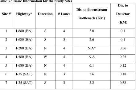
Based on the three criteria above, seven on-ramp bottlenecks were selected as the
study sample. Two of the sites are in the San Antonio area, and the remaining five are from
the Bay area. The basic information for each on-ramp bottleneck site is summarized in Table
3.3.
Table 3.3 Basic Information for the Study Sites
Site # Highway* Direction # Lanes
Dis. to downstream Bottleneck (KM)
Dis. to Detector
(KM)
1 I-880 (BA) S 4 3.0 0.1
2 I-680 (BA) S 3 2.6 0.1
3 I-280 (BA) N 4 N.A* 0.36
4 I-580 (BA) W 4 N.A 0.25
5 I-680 (BA) N 4 6.1 0.12
6 I-35 (SAT) N 3 3.6 0.18
7 I-35 (SAT) S 3 2.2 0.38
3.2 Breakdown Determination
Breakdown determination is the critical starting point for both stochastic capacity and
queue discharge studies. As mentioned earlier, although most previous studies used speed as
the threshold, a single speed threshold was not considered appropriate for determining
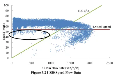
congested conditions based on the speed-flow diagram from field data. Figure 3.2 shows 21
months of 15‐minute freeway data from the I-880 in Bay Area in CA. The horizontal line
superimposed on the plot indicates the speed boundary that was used to isolate congested
conditions. As is apparent from the graph, a single speed threshold was not considered
sufficient for determining congested conditions. Observed conditions exhibiting a flow rate
lower than 1000 vph per lane but with speeds higher than 40 mph were considered to be
reflective of anomalous free‐flow conditions rather than congested conditions. The data
pattern shown in Figure 3.2 is typical of the seven on-ramp sites, and the presence of low
flow observations below the critical speed threshold creates the need for a robust phase
Figure 3.2 I-880 Speed Flow Data
Therefore, a combination of speed and density (diagonal line in Figure 3.2) threshold
was applied to identify congested conditions, thereby avoiding the inclusion of anomalous
low speed data such as the observations identified within the oval in Figure 3.2. The
observed traffic states are considered to represent congested conditions only when:
a) The observed speed is below the critical speed AND
b) The observed density is greater than or equal to boundary between level of service C
and D (LOS C/D).
As mentioned above, the critical speed and the density at the LOS C/D boundary are
locally calibrated for each of the specific study sites. The procedure for calculating these site
specific thresholds is described in the following paragraphs.
LOS C/D
First, 15-minute flow rate values, q, in the top one percentile tail are identified. The
average of this sample of near maximum flows was found to be generally equivalent to the
traditional capacity defined in the HCM. Secondly, the density for each 15-minute
observation is then calculated by:
̅ (3-1)
Where,
k: Density for each 15-min. observation (veh/mi/ln)
q: 15-min. flow rate for the top one percentile flows (veh/h/ln)
̅: Space mean speed (mph)
The critical speed is then calculated as:
critical
q u
k
(3-2)Where,
q: 15 min. flow rate in the top one percentile flows;
k: 15 min. density corresponding to flow q.
The equivalent density at capacity based on HCM definition is calculated by
∑ (3-3) Where,
Finally, the adjusted HCM-based, critical density threshold (LOS C/D boundary) is calculated by
(3-4)
Where,
26 pc/mi/ln represents the maximum density per lane passenger car equivalent density for
LOS C for basic freeway segments per HCM 2000
45 pc/mi/ln respresents the corresponding per lane passenger car density at capacity
It should be noted that the equation above provides adjusted values for the LOS C/D
thresholds based on the observed density at capacity. In summary, traffic condition
observations are identified as representing congested flow when the observed 15-minute
speed, , is less than the critical speed, Critical , and the observed 15-minute density,
̅, is greater than the critical density, kCritical, as specified in Equation 3-2 and 3-4,
respectively.
Each of the study sites was analyzed independently. At each site, the speed and
vehicle count data were summarized in 15-min. intervals across all lanes. The vehicle count
data were then expressed as equivalent hourly flow rates per lane. Based on the above
methodology, the traffic parameters for each study site are summarized in Table 3.4. The
corresponding flow-speed curves (Appendix B) for each study site were plotted and
illustrated for three different traffic states (“Free Flow”, “Congestion”, and “Pre-Breakdown
Flow”).
Table 3.4 Calibrated Traffic Parameters for Each Study Site Site # Highway
Average Top 1 percentile Flow Rate (veh/h/ln)
Critical Speed (mph)
Density (C/D) (veh/mi/ln)
1 I-880 (BA) 2052 56 21
2 I-680 (BA) 2093 53 23
3 I-280 (BA) 2183 53 24
4 I-580 (BA) 1982 49 23
5 I-680 (BA) 2127 54 23
6 I-35 (SAT) 1992 47 23
7 I-35 (SAT) 2172 63 20
In order to ensure the identified breakdown was not due to the downstream queue
spillback, traffic data from the next downstream sensor were also analyzed following the
same procedure above. The breakdown observations at the study sites were screened out
from the study sample whenever there were simultaneous downstream breakdown
observations. Moreover, based on the information provided by PeMS, there is no long-term
work zone closure to the study sites during the analysis period.
Taking traffic observations of site 1 on January 3rd , 2007 from 15:00 to 18:15 as an example, the way how pre-breakdown flow rate and breakdown are identified is
demonstrated in Figure 3.3. Based on the speed and density of the traffic observations at 15
speed is below the critical speed (56 mph in this example) and the observed density is greater than or equal to boundary between level of service C and D (21 veh/mi/ln in this example).
The uncongested state just preceding the breakdown state (highlighted in yellow cycle) is
then identified as pre-breakdown flow rate.
Figure 3.3 Illustrations of the Identification of Pre-breakdown and Breakdown
3.3 Models for Stochastic Capacity and Queue Discharge
The introduction of stochastic capacity at critical points within the network that suffer
from queue and congestion more frequently, i.e. freeway bottlenecks and signalized
intersections, enables reasonable and realistic modeling of travel time variability and the
two basic traffic states in uninterrupted freeway operation: uncongested and congested flow.
In defining stochastic capacity, the focus lies on the pre-breakdown state, i.e., the
uncongested states just preceding the breakdown state. Once the breakdown states were
identified, all the corresponding pre-breakdown states were selected from each data set.
However, it should be noted that it is important to exclude the pre-breakdown flow rate under
non-recurring conditions as much as possible. The possible impacts of severe weather and
incidents should be screened from the dataset. Regarding the impacts of incidents, if an
incident occurs between the target sensor and the next downstream sensor, the corresponding
pre-breakdown observations should be excluded. Based on the incident logs provided by
PeMS, several pre-breakdown observations were excluded from the dataset. Unfortunately,
Transguide does not provide any incident information, which prevents us to screen out the
impacts of incident on the three study site in San Antonio. Moreover, the two-year weather
data were also downloaded from weatherundergroud.com. When there are unrecursive
conditions, such rain, snow, and poor visibility, the corresponding pre-breakdown
observations were also identified and then removed from the dataset of pre-breakdown
observations. The criteria used to remove unrecursive pre-breakdown observations are:
1. Precipitation > 0 mm OR
2. Wind speed > 16 mph OR
Table 3.5 summarizes the number of unrecursive pre-breakdown observations
screened by above criteria and the number of recursive pre-breakdown observations for
develop stochastic capacity models.
Table 3.5 Summary of Pre-breakdown Observations Screening Results
Site # Highway Incident Precipitation Wind Visibility Pre-breakdown
1 I-880 (BA) 42 110 137 13 1436
2 I-680 (BA) 17 29 30 5 511
3 I-280 (BA) 16 51 84 8 619
4 I-580 (BA) 28 22 42 5 994
5 I-680 (BA) 5 86 251 11 604
6 I-35 (SAT) N.A. 64 93 20 377
7 I-35 (SAT) N.A. 68 82 17 372
Based on Table 3.5, it seems that incident and visibility have fewer impacts on the
quality of the sample of pre-breakdown observation than the precipitation and wind.
Therefore, it is necessary to account for the potential weather impacts in order to study the
stochastic capacity under recursive condition.
For the sites discussed above, heavy vehicle count data was not available. Therefore,
the HCM 2000 default of 5% heavy vehicles and the level general freeway segment
PeMS data to passenger car equivalent flow rates. It should be acknowledged that such
assumptions could be a cause of the variation of pre-breakdown flow rates as well and
therefore may bias the analysis result and model development. The only way to address this
issue is to use the sensor data with vehicle classification, although it really depends on the
real-world traffic monitoring system. It should also be noted that by using the data with
vehicle classification and then excluding the impact of heavy vehicles (refer to Chapter 5),
the values of pre-breakdown flow rates still vary in a wide range.
Due to the lack of the incident logs and weather information, a statistical approach
was initially proposed to exclude outlying pre-breakdown flow rates. A pre-breakdown flow
rate q, is identified as an outlier if:
(3-5)
Where,
Q0.75: 75thpercentile flow rate (pc/h/ln);
Q0.25: 25th percentile flow rate (pc/h/ln);
IQR: Q0.75 -Q0.25.
The speed-flow diagram in Figure 3.4 shows the pre-breakdown and outlier
observations for one study site (I-880). Almost all of flow rates above the HCM equivalent
LOS C/D density boundary were identified as outliers. For the 15 minute aggregated traffic
data, it looks reasonable that the pre-breakdown flow rates would not occur at LOS C or
the screening results above, only 56% of the unrecursive pre-breakdown observations were
identified as the outliers for this specific study site. It may suggest that the simplified
statistical method is not sufficient to screen out the impacts of unrecursive pre-breakdown
observations when people try to develop the stochastic capacity model and carefully
examining the incident logs and weather information is necessary.
Figure 3.4 Pre-breakdown Flows and Outliers for I-880
3.3.1 Stochastic Capacity Model for Freeway On-ramp Bottlenecks
After removing the possible outliers, the remaining pre-breakdown flow rates were
then used to develop the probability distributions that reflect the stochastic characteristics of
freeway average pre-breakdown headway. The most common tests for goodness-of-fit are the