Available Online atwww.ijcsmc.com
International Journal of Computer Science and Mobile Computing
A Monthly Journal of Computer Science and Information Technology
ISSN 2320–088X
IMPACT FACTOR: 5.258
IJCSMC, Vol. 5, Issue. 5, May 2016, pg.110 – 116
Enhanced of Image Mining Techniques the
Classification Brain Tumor Accuracy
(ENCEPHALON)
Prof. P.Senthil
MA.,PGDCA.,M.Sc.,MPhil.Associate Professor in MCA Computer Science, Kurinji College of Arts and Science, Tiruchirappalli-620002, India
Email: [email protected]
Abstract: Image Mining is growing modernly outstanding to its wide applications. An efficient MRI image segmentation is needed at present. In this paper, MRI Brain segmentation is done by Semi supervised learning which does not require pathology modeling and, thus, allows high degree of a utomation. In abnormality detection, a vector is characterized as anomalous if it does not comply with the probability distributio n obtained from normal data. The estimation of the probability density function, however, is usually not feasible due to large data dimensionality. In order to overcome this challenge, we treat every image as a network of locally coherent image partitions (overlapping blocks). We formulate and maximize a strictly concave likelihood function estimating abnormality for each partition and fuse the local estimates into a globally optimal estimate that satisfies the consistency c onstraints, based on a distributed estimation algorithm. After this features are extracted by Gray-Level Co-occurrence Matrices (GLCM) algorithm and those features are given to Particle Spam Optimization (PSO) and finally classification is done by using Library Support Vector Machine (LIBSVM).Thus results are evaluated and proved its efficiency using accuracy.
Keywords: Gray-Level Co-occurrence Matrices, Image Mining, Image Segmentation, Spam Optimization, Support Vector Machine.
INTRODUCTION
Image segmentation is an significant process in image processing. They are used in various applications like biomedicine, remote sensing, control of quality and many others. The main aim of segmentation of image is to extract information from the images to make out different objects of significance. The segmented image separates abnormal area and normal area or differentiates the objects etc.
In medical image segmentation, Brain , retina, breast, kidney and liver based image segmentations are the active area of research based on image processing.
The anatomy of the Brain is complex due its complicate structure and function [1]. The Brain is the part of the central nervous system. It is the centre to control the mental processes and physical action of a human being. Brain abnormality is a symptom where motor impairment and neuropsychological problems affect the central nervous system. It is an abnormal growth of cells within the Brain , which can be cancerous or non-cancerous [2]. To date, numerous researches of Brain abnormality detection had been conducted due to its important roles in identifying anatomical areas of interest for diagnosis, treatment, or surgery planning paradigms [3].
Magnetic Resonance Imaging (MRI) is a primary medical imaging modality that commonly uses to visualize the structure and the function of human body [4]. It provides rich
information for excellent soft tissue contrast which is especially useful in neurological studies [5]. In previous years, MRI is observed to play an important role in Brain abnormalities research in determining size and location of affected tissues [6].
Image segmentation refers to a process of assigning labels to set of pixels or multiple regions [7]. It plays a major role in the field of biomedical applications as it is widely used by the radiologists to segment the medical images input into meaningful regions. Thus, various segmentation techniques in medical imaging depending on the region of interest had been proposed [8].
Arduini et al. solved two problems, restoration of SAR images and extraction of intensity discontinuities, by using two distinct MRFs. Held et al. used one added MRF, i.e., the bias field, to sweep the obstacle of MRI Brain segmentation but they did not couple the two MRFs compactly because the two fields are assumed independent.
This work makes two fundamental contributions in discovering abnormality. First, an objective function is defined that evaluates probability of the test data according to a statistical model of normal data in a lower dimensional space, and also exploits similarity with the model representation as well as similarity with the original data. The objective function minimization is formulated as a quadratic optimization problem. Second, the curse of dimensionality is tackled by proposing a scheme where an image is partitioned into a set of overlapping blocks at various locations, similarly The objective function is optimized for each local subspace and then the local subspace estimates are fused into a globally optimal estimate that satisfies coupling constraints. Data fusion is performed by applying a distributed estimation algorithm based on dual decomposition decomposition and developed for solving large-scale problems. The proposed approach is comprehensively evaluated using receiver operating characteristic (ROC) analysis.
The paper is organized as follows. Section II gives the relation work. In Section III, presents the proposed work. Then results are presented in Section IV followed by conclusion in Section V.
RELATED WORKS
Atlas-guided [19] approaches are an effective tool for medical image segmentation when a standard atlas or template is available. The atlas is generated by compiling information on the anatomy that requires segmenting. This atlas is then used as a reference frame for segmenting new images. It first finds a one-to-one transformation that maps a pre-segmented atlas image to the target image that requires segmenting. This process is often referred to as atlas warping.
An automatic image segmentation method using thresholding technique. This is based on the assumption that adjacent pixels whose value (grey level, color value, texture, etc) lies within a certain range belong to the same class and thus, good segmentation of images that include only two opposite components can be obtained. Threshold based image segmentation are Global Thresholding, Local Thresholding, and Adaptive Thresholding. The key parameter in image segmentation using thresholding technique is the choice of selecting threshold value T.
There are two types Segmentation [14] -Soft Segmentation and Hard Segmentation. Segmentations that allow regions or classes to overlap are called soft segmentations. Soft segmentations are important in medical imaging because of partial volume effects, where multiple tissues contribute to a single pixel or voxel resulting in a blurring of intensity across boundaries [14]. A hard segmentation forces a decision of whether a pixel is inside or outside the object or class. Soft segmentations based on membership functions can be easily converted to hard segmentations by assigning a pixel to its class with the highest membership value. Automated segmentation and delineation of detailed structures remains a difficult task in MRI segmentation.
Clustering algorithms essentially perform the same function as classifier methods without the use of training data. Thus, they are termed unsupervised methods. Two commonly used clustering algorithms are the k -means [23], the fuzzy c-means algorithm. The K-means clustering algorithm clusters data by iteratively computing a mean intensity for each class and segmenting the image by classifying each pixel in the class with the closest mean and fuzzy c-mean [22]has membership function based on membership values it divides pixel into different classes which is also iterative based method.
PROPOSED WORK
The methodology for abnormality segmentation here uses 1) a set of pathology-free images in order to calculate an objective function measuring similarity to a healthy Brain and 2) a test image which contains both normal and abnormalities for which the objective function is maximized. All images are co registered and the mean image is calculated and subtracted from them. The solution is based on partitioning the spatial domain into overlapping, equally sized blocks in random locations. The algorithmic steps are the following. First, the test image is scanned and a random block is selected (among the not already scanned locations).
By concatenating the image intensities in the block, the test vector is constructed, where d is the number of dimensions (e.g., number of voxels in the block). The same block is then extracted from all pathology-free images forming the training vectors where n is the number of subjects. The training set V is used to calculate an objective function ( ) the optimization of which gives a new vector the optimization of which gives a new vector ̂ that is “less abnormal” and also as similar as possible to the original vector . However, since the blocks are overlapping, the solutions cannot be independently calculated for each block. After merging the solutions of all blocks, a spatial abnormality score map is calculated for the whole image by subtracting the reconstructed image from the original one.
A. Formulation of the Objective Function
Since anomalies are defined as points with low probability density, it is expected to estimate ̂ by maximizing the pdf obtained for the normal data. However, if the vector is high dimensional, the estimation of the pdf is not feasible. Therefore, we will maximize the pdf in a lower dimensional space ( ) where is the representation of in a basis :
Here, x is a column vector assumed to be centered at the origin and T denotes the matrix transpose. If the Karhunen–Loeve (KL) transform (or PCA) is applied, the basis is formed by
the ( ) matrix of the eigenvectors of the covariance
matrix of the training set V, i.e, . / The KL transform can be inverted as follows:
Assuming that x follows a multivariate Gaussian distribution, the density of u is the multivariate Gaussian density:
( )
( )
. /
eigen values , with are zero and the corresponding eigenvectors in are ignored. If all other eigenvectors are retained
According to previous equation, ( ) is maximized when . / is minimized. Based on maximization of the density in respect to x then is equivalent to minimizing the following term:
( ) ( ( ) )
Since u is lower dimensional than x, there exist an infinite number of data points with the same function cost value in above equation. In order to reduce the solution space, we use an additional term that constraints the solution to remain close to the subspace spanned by W. If the test vector is , then its projection on is
The second energy term expresses the distance to the projected point :
( ) ‖ ‖ ( ) ( )
Where ‖ ‖ denotes the -norm. If , this term expresses the reconstruction error or residual. Since does not necessarily lie within the subspace spanned by W, this term is larger than zero in this setting. This happens mainly because the abnormal vector is inconsistent with the normal data building the basis . Generally by minimizing , we infer that x becomes sufficiently linearly dependent on the current dictionary (normal data), and represents normal behavior. The first two terms statistically model normality and are used to make the image look like if abnormality were removed. The final term is used to constrain the reconstructed image to be as similar as possible to the original image based on the assumption that the majority of the voxels in the test image are normal. If all voxels are equally possible to be abnormal, then the distance from can be used as dissimilarity criterion:
( ) ‖ ‖ ∑( ( ) ( ))
Where j indicates the voxels in the image.
If prior knowledge exists on spatial locations of possible abnormality, then weights can be incorporated to penalize less the dissimilarity in those locations. Since this method is unsupervised for the abnormal class and aims to generalize for any kind of abnormality, we do not incorporate a prior for the abnormal areas. However, we focus on the normal class and introduce a confidence measure on the estimation ability of the calculated statistical model. Regions with large variability are much more difficult to model than uniform areas. A confidence map or vector shows the degree of certainty we have on the reconstruction of each parameter ( ) Parameters with high uncertainty in estimation should not deviate significantly from their original values ( ). This is achieved by penalizing any change on those parameters more than on other parameters. By incorporating an uncertainty vector
the third term becomes
( ) ( ) ( )
Where A is a ( ) diagonal matrix with normalized elements ∑ ( ) ( )
on the main diagonal. The uncertainty vector a is calculated as the average reconstruction error at each
location over all training images obtained by leave-one-out cross validation:
∑ √
( )
Where is the basis formed without using training image The previous three terms are combined into a single objective function, ( ) by using different weights, shown as follows:
( )
Where, ( ) ( ) ( ) ( ) And
and
According to the values of the weights, we balance between the model term (including and ), controlling the similarity with the training set consisting of normal data, and the data term ( ), controlling the similarity with the original vector. The weights depend on the confidence we have on the statistical model, as well as on the dominance of novelty or anomaly over the data. The larger the anomaly, the smaller should be the contribution of the data term. The model term on the other hand should always contribute significantly to the solution since it guides toward normality. The weights can be empirically determined by maximizing segmentation accuracy through cross validation on labeled data.
Once the optimization problem is solved, the final reconstructed image is created by recentering to the original space, i.e., by adding the mean image to the result.
B. Optimization of the Objective Function
The objective function can be written in the form of a quadratic programming problem without any linear (equality or inequality) constraints
( ) ( )
Subject to
Where lower and upper bounds on x, H are is a ( ) positive semi definite symmetric matrix, and f is a d-element column vector.
( )
*( ) -
Where I is the ( ) identity matrix,
( ) is the inverse diagonal matrix of the
largest eigenvalues retained and the matrix of the corresponding retained eigenvectors.
C. Distributed Estimation
The maximum likelihood estimation problem in a distributed setting is solved using dual decomposition based on the algorithm. Let us assume that blocks (partitions) are extracted from an image and that the blocks are coupled through consistency constraints that require the image intensities in overlapping voxels to be equal. The variables that are constraint to be equal across different blocks are denoted as public variables. The variables that are local to each block and are not common in other blocks are denoted as private variables.
The public variables for all blocks are collected together into one vector variable ( ) where
, is the total number of public variables. A vector
is introduced to give the common values of the
public variables in each consistency constraint. The constraints are expressed as
y =
where specifies the set of coupling constraints for the given block interaction
{ ( )
Lagrange multipliers are introduced for the coupling constraints and a projected sub gradient method is used to solve the dual master problem. Using these dual variables, optimization is independently performed in each block, and later on, the net variables are updated using the optimal values of the public variables of the blocks adjacent to that net. The dual variables are then updated, in a way that brings the local copies of public variables into consistency.
A measure of the inconsistency of the current values of the public variables (consistency constraint residual) is given by the norm of the vector computed in the last step, ̂
D. Implementation
The optimization for each block can be as a quadratic programming problem in respect to where the log likelihood function is given by the negative objective function.
In order to extract from , the matrix [
], where is composed of zeros and is the identity matrix, is the identity matrix, such that
Then the equation becomes,
( ( ) )
( ( ) )
( )
Where and is calculated for block and
.
E. Independent Component Analysis(ICA)
The ICA segmentation is efficient segmentation which is used before feature extraction here.
ICA of a random vector consists of estimating the following generative model for the data:
where the latent variable (components) in the vector
( ) are assumed independent. The matrix A is
a constant „mixing‟ matrix.
This is the simplest and widest used definition in most research on ICA. There are also other ICA definitions, which can be found in the literature [24,25].
To maximize by stochastic gradient ascent the joint entropy
( ( )) of the linear transform squashed by a sigmoidal
function g. The updating formula for is:
( ( ) )
Where and ( ) ( ) is calculated for each
component of . Before the learning procedure, is sphered by subtracting the mean and multiplying by a whitening filter:
,( )( ) - ( )
This gives the segmented image from which features are extracted.
F. Feature Extraction:
The features are important for every classification algorithms. Here texture features of images are extracted.
The GLCMs features are stored in a matrix, where is the number of GLCMs calculated usually due to the different orientation and displacements used in the algorithm. Usually the values and are equal to 'NumLevels' parameter of the GLCM computing function. Note that matlab quantization values belong to the set * + and not from * ( )+ as provided.
The following GLCM features are extracted:
Autocorrelation
Contrast
Correlation
Correlation
Cluster Prominence
Cluster Shade
Dissimilarity
Energy
Entropy
Homogeneity
Homogeneity
Maximum probability
Sum of squares
G. Classification:
The classification of abnormality and normality is improved here by using PSO with LSVM technique.
I. Particle swarm optimization
Particle swarm optimization (PSO) is a population-based optimization algorithm modeled after the simulation of social behavior of birds in a flock [12]. The algorithm of PSO is initialized with a group of random particles and then searches for optima by updating generations. Each particle is flown through the search space having its position adjusted based on its distance from its own personal best position and the distance from the best particle of the swarm. The performance of each particle, i.e. how close the particle is from the global optimum, is measured using a fitness function which depends on the optimization problem.
Each particle i flies through an n-dimensional search space, and maintains the following:
the current position of ith particle (x-vector)
the personal best position of ith particle (p-vector), and , the current velocity of ith particle (v-vector).
The personal best position associated with a particle, is the best position that the particle has visited so far. If denotes the fitness function, then the personal best of at a time step is updated as:
( ) * ( ) ( ( )) ( ( ))
( ) ( ( )) ( ( ))
* ( ) ( ) ( )+
{ ( ( )) ( ( )) ( ( ))+ The velocity updates are calculated as a linear combination of position and velocity vectors. Thus, the velocity of particle is updated and the position of particle is updated by the following equations.
( ) ( ) ( ( ) ( ))
( ( ))
( ) ( ) ( )
In the formula, is the inertia weight [26], and are the acceleration constants, and are random numbers in the range [0,1] and must be in the range , - where is the maximum velocity.
II. Library Support Vector Machine:
LIBSVM is a library for Support Vector Machines (SVMs). The goal is to easily apply SVM to their applications. LIBSVM has gained wide popularity in machine learning and many other areas. In this work, we present implementation of LIBSVM. Issues such as solving SVM optimization problems theoretical convergence multiclass classification probability estimates and parameter selection.
A typical use of LIBSVM involves two steps: first, training a data set to obtain a model and second, using the model to predict information of a testing data set. For SVC and SVR, LIBSVM can also output probability estimates.
This is same as SVM technique, where in training SVM the An m by 1 vector of training labels (type must be double) is taken.
Then parameters for gamma in LIBSVM are taken from PSO algorithm. And the Cost parameter is set as the parameter C of C-SVC is taken.
Kernels:
Kernel methods in general have gained increased due to the grown of popularity of the Support Vector Machines. Support Vector Machines are linear classifiers and regressors that, through the Kernel trick, operate in reproducing Kernel Hilbert spaces and are thus able to perform non-linear classification and regression in their input space.
Here Radial Bias Function Kernel is used and it is expressed as
(
‖ ‖ )
And detailed discribtion is given in [28]. This is given as kernel in LIBSVM technique. By this the classification of abnormal and normal MRI Brain images is performed and their affected disease is identified.
EXPERIMENTAL RESULTS
The experiment is done to evaluate the performance of this proposed work. The MATLAB environment is chosen and MRI images are collected from various Scan centers. Here three major diseases type of Astrocytoma, Giloma and Metastasis and abnormality of dyaplasia and Brain infraction is identified.
The input image is preprocessed and features are extracted from it. The extracted features are given for the PSO algorithm which helps in finding the parameters for the LIBSVM classification.
Figure 3.1: Input Image-1 Figure 3.2: Segmented Output
Figure3.3: Identified of Affected Area
Figure 3.4: Output Result
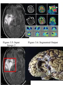
Figure 3.5: Input Image-2
Figure 3.6: Segmented Output
Figure3.7: Identified of Affected Area
Likewise for other diseases and abnormalities are identified by using this technique.
H. Performance Evaluation:
The classification accuracy is measured here by the MRI Brain image database. The input database consists of MRI Brain images containing diseases of Astrocytoma, Giloma and Metastasis. And fracture of Brain infraction and dyaplasia.
The table 1 shows that proposed algorithm of PSO with LIBSVM produces best accuracy for the Metastasis, Brain infraction and dyaplasia. And better results for Giloma for the input images.
CONCLUSION
The identification and detection of abnormality and diseases in Brain is carried here by MRI Brain images. The proposed work is done by extracting GLCM features and given to the PSO. The PSO is efficient technique for segmentation which finds the parameters for the classification technique. The classification technique of Library SVM is used which is improved technique than traditional SVM in which RBF kernel is used to boost the classifier. The performance of this work is measured by accuracy calculation for three Brain diseases and two tractors which proves the nearly maximum results. In future large database can be taken for evaluation with more number of Brain images.
ACKNOWLEDGEMENT
This paper is made possible through the help and support from everyone, including: My wife M.suganya and Daughter S.S.Inakshi and My sir S.Syed Nazimuddeen and S.Irshath Ahamed , and in essence, all sentient beings. I sincerely thank to my parents, family, and friends, who provide the advice and financial support. The product of this paper would not be possible without all of them.
REFERENCES
[1] G. Evelin Sujji, Y.V.S. Lakshmi, G. Wiselin Jiji,” MRI Brain Image Segmentation based on Thresholding “,International Journal of Advanced Computer Research (ISSN (print): 2249-7277 ISSN (online): 2277-7970) Volume-3 Number-1 Issue-8, March-2013, pp.97-101. [2] Dusan Hirjak, Katharina M. Kubera, Robert C. Wolf,
Anne K. Thomann, Sandra K. Hell, Ulrich Seidl, Philipp A. Thomann Local brain gyrification as a marker of
neurological soft signs in schizophrenia Behavioural Brain Research,Volume 292, 1 October 2015, Pages 9-25 [3] So Young Chang, Ji Hoon Park, Young Ho Kim, Jong
Seong Kang, Ji-Young Min A natural component from Euphorbia humifusa Willd displays novel, broad-spectrum anti-influenza activity by blocking nuclear export of viral ribonucleoprotein Biochemical and Biophysical Research Communications, Volume 471, Issue 2, 4 March 2016, Pages 282-289
[4] Ji Hoon Park, Eun Beul Park, Jae Yeol Lee, Ji-Young Min Identification of novel membrane-associated prostaglandin E synthase-1 (mPGES-1) inhibitors with anti-influenza activities in vitro Biochemical and Biophysical Research Communications, Volume 469, Issue 4, 22 January 2016, Pages 848-855
[5] Petra Perner Tracking Living Cells in Microscopic Images and Description of the Kinetics of the CellsOriginal Research Article Procedia Computer Science, Volume 60, 2015, Pages 352-361
[6] Angela Lausch, Andreas Schmidt, Lutz Tischendorf Data mining and linked open data – New perspectives for data analysis in environmental research Ecological Modelling, Volume 295, 10 January 2015, Pages 5-17
[7] Hee-Young Kim, Sunju Kong, Sangmi Oh, Jaewon Yang, Eunji Jo, Yoonae Ko, Soo-Hyun Kim, Jong Yeon Hwang, Rita Song, Marc P. Windisch Benzothiazepinecarboxamides: Novel hepatitis C virus inhibitors that interfere with viral entry and the generation of infectious virions Antiviral Research, Volume 129, May 2016, Pages 39-46
[8] Joo Hwan No Visceral leishmaniasis: Revisiting current treatments and approaches for future discoveries Acta Tropica, Volume 155, March 2016, Pages 113-123. [9] Michael Osadebey, Nizar Bouguila, Douglas Arnold
Chapter 4 - Brain MRI Intensity Inhomogeneity Correction Using Region of Interest, Anatomic Structural Map, and Outlier Detection Applied Computing in Medicine and Health, 2016, Pages 79-98.
[10] Tejas Sankar, M. Mallar Chakravarty, Agustin Bescos, Monica Lara, Toshiki Obuchi, Adrian W. Laxton, Mary Pat McAndrews, David F. Tang-Wai, Clifford I. Workman, Gwenn S. Smith, Andres M. Lozano Deep Brain Stimulation Influences Brain Structure in Alzheimer's DiseaseBrain Stimulation, Volume 8, Issue 3, May–June 2015, Pages 645-654.
[11] Chinnu “A MRI Brain Tumor Classification Using SVM and Histogram Based Image Segmentation” Chinnu A/ (IJCSIT) International Journal of Computer Science and Information Technologies, Vol. 6 (2) , 2015, 1505-1508. [12] Hojin Ha, Dongha Hwang, Guk Bae Kim, Jihoon Kweon,
Sang Joon Lee, Jehyun Baek, Young-Hak Kim, Namkug Kim, Dong Hyun Yang Estimation of turbulent kinetic energy using 4D phase-contrast MRI: Effect of scan parameters and target vessel size Magnetic Resonance Imaging, Volume 34, Issue 6, July 2016, Pages 715-723. [13] Nicolas Chauffert; Pierre Weiss; Jonas Kahn; Philippe
Ciuciu; A projection algorithm for gradient waveforms design in Magnetic Resonance Imaging,IEEE Transactions on Medical Imaging Year: 2016, Volume: PP,Issue:99,Pages:1- 1, DOI: 10.1109/TMI.2016.2544251 [14] Vladimir Golkov; Alexey Dosovitskiy; Jonathan Sperl;
AUTHOR’S BIOGRAPHIES