Changing Points in APN Functions
Lilya Budaghyan, Claude Carlet, Tor Helleseth, Nikolay Kaleyski
Abstract
We investigate the differential properties of a construction in which a given functionF :F2n→F2nis modified atK∈Npoints in order to obtain a new functionG. This is motivated by the question of determining the minimum Hamming distance between two APN functions and can be seen as a generalization of a previously studied construction in which a given function is modified at a single point. We derive necessary and sufficient conditions which the derivatives of F must satisfy for G to be APN, and use these conditions as the basis for an efficient filtering procedure for searching for APN functions whose value differs from that of a given APN functionF at a given set of points. We define a quantitymF related toF counting the number of derivatives of a given type, and derive a lower bound on the distance between an APN functionF and its closest APN neighbor in terms ofmF. Furthermore, the valuemF is shown to be invariant under CCZ-equivalence and easier to compute in the case of quadratic functions. We give a formula formF in the case ofF(x) =x3 which allows us to express a lower bound on the distance betweenF(x)and the closest APN function in terms of the dimension nof the underlying field. We observe that this distance tends to infinity with n. We also compute mF and the distance to the closest APN function for a representativeF from each of the switching classes overF2n for4≤n≤8.
For a given functionFand valuev, we describe an efficient method for finding all sets of points{u1, u2, . . . , uK} such that settingG(ui) =F(ui) +vand G(x) =F(x)forx6=uiis APN.
I. INTRODUCTION
A vectorial (n, m)-Boolean function is any mapping F : F2n → F2m, where F2n is the finite field with 2n
elements. Such a function can also be seen as mapping sequences of nbits (zeros and ones) to sequences of m
bits, which more clearly underlines their practical importance. Vectorial Boolean functions are of central interest in
cryptography since they represent the most important part of many encryption algorithms: for instance, the Advanced
Encryption Standard (AES) and algorithms based on Feistel networks such as the Data Encryption Standard (DES),
all utilize vectorial Boolean functions in the role of so-called “substitution boxes” (see e.g. [18] for basic background
on cryptography and encryption schemes). The resistance of the encryption to various categories of cryptanalytic
attacks then directly depends on the properties of the underlying Boolean functions.
Almost Perfect Nonlinear (APN) functions were introduced by Nyberg [16] as the functions that provide optimal
resistance to the so-called differential attack invented by Biham and Shamir [2]. More precisely, we say that a
functionF:F2n→F2n is APN if the equationF(x) +F(x+a) =binxhas at most2solutions for anya∈F∗2n
and any b∈F2n. Despite the simplicity of this definition, finding new examples of APN functions, even in finite
fields of relatively low dimension and investigating their properties is a challenging task, due to which various
methods of constructing such functions have been examined by researchers.
In [5], a construction in which a given functionF :F2n→F2n is modified at one point is examined, motivated
nonexistence results are obtained in that paper, which support the conjecture that this is impossible. The idea of
this construction is interesting in its own right, however, and it can naturally be generalized to the modification of
more than one point.
The particular case of swapping, or exchanging, two points of a given function is already studied [19] in the
context of constructing differentially 4-uniform permutations. The more general question of arbitrarily modifying
the values of a given function at two points, as well as the construction of swapping two points in a more general
context is investigated in [14]. Two main characterizations of the APN-ness of the modified function are obtained,
one in terms of the power moments of the Walsh transform, and one in terms of the differential properties of the
original function. We observed that if F and G are at distance two, then at most one of F and G can be AB,
and at most one of them can be plateaued; furthermore, if the algebraic degree of say F is less than n−1, then
Gcan be neither AB nor plateaued (except for some trivially small dimensions of the finite field). In the case of
swapping the values of a function at0and1, we obtained a sufficient condition for disproving the APN-ness ofG
by computing a lower bound on the sum P
y∈F2n∆F(y, F(y) + 1) + ∆F(y+ 1, F(y)). We also showed how to
compute a lower bound on this quantity in the case of power functions.
In this paper, we consider the general case of arbitrarily changingKpoints. To be more accurate, given a function
F :F2n →F2n, some K distinct field elements u1, . . . , uK ∈F2n and someK elements v1, v2, . . . , vK ∈F∗2n,
we defineGas
G(x) =
F(ui) +vi x=ui
F(x) x /∈ {u1, u2, . . . , uK}
and try to find some correlation between the properties of F and those of G. We derive sufficient and necessary
conditions that the derivatives ofF must satisfy in order forGto be APN, and obtain an efficient filtering procedure
for finding all possible values of v1, v2, . . . , vK in the case that u1, u2, . . . , uK are known. In the case when F is
itself APN, we define the value mF, which counts the number of derivatives ofF satisfying a certain condition,
and express a lower bound on the distance betweenF and the closest APN function in terms of mF. We further
demonstrate thatmF is invariant under CCZ-equivalence and that its computation is particularly efficient whenF
is quadratic. In addition, we show how an exact formula formF can be computed in the case ofF(x) =x3, and
experimentally computemF for representatives from all switching classes in [13].
In the case when v1 = v2 = · · · = vK, we show how all possible combinations of points u1, u2, . . . , uK
can be found (for all values of K) by solving a system of linear equations. Note that constructions of the form
G(x) =F(x) +vf(x)for f :F2n→F2 have been investigated in [6], [13].
II. PRELIMINARIES
A. Representation of Vectorial Functions
Given two positive integers n and m, a vectorial Boolean (n, m)-function, or simply (n, m)-function, is any
functionF :Fn
2 →Fm2 . It can be uniquely expressed in the so-calledalgebraic normal form(ANF) as follows [8]:
F(x1, x2,· · · , xn) =
X
I⊆{1,2,...,n} aI(
Y
i∈I
xi) =
X
I⊆{1,2,...,n}
Thealgebraic degreeof F(x1, x2,· · · , xn)is defined as the degree of its ANF, namely
deg(F) = max{|I|:aI 6= (0,0,· · · ,0), I⊆ {1,2,· · ·, n}}.
Clearly,deg(F)≤n.
Vectorial Boolean(n,1)-functions, i.e. functions of the formf :F2n→F2, are called simplyBoolean functions.
When m =n it is often more convenient to identify the vector space Fn2 with the finite fieldF2n. Note that
any basis{e1, e2,· · ·, en} for F2n, viewed as a vector space overF2, determines a correspondence between F2n
and Fn2 via x=
Pn
i=1xiei. The algebraic degree does not depend on the choice of the basis since any change of basis corresponds to a linear permutation. Then any(n, n)-function has a unique representation as a univariate
polynomial over F2n of the form
F(x) =
2n−1
X
i=0
aixi, ai ∈F2n.
Letx=Pn
i=1xiei andi=P n−1
s=0is2s whereis∈ {0,1}. ThenF can be rewritten as
F(x) =
2n−1
X
i=0
ai n
X
i=1
xiei
!i
=
2n−1
X
i=0
ai n−1
Y
s=0
n
X
i=1
xie2 s i
!is
which is exactly the ANF of F. Moreover, let w2(i) =Pns=0−1is denote the2-weight ofi, where0≤i≤2n−1 has binary expansioni=Pn−1
s=02
si
s. Then the algebraic degree ofF in univariate polynomial form is equal to
deg(F) = max{w2(i) :ai = 0,6 0≤i≤2n−1}.
B. Almost Perfect Nonlinear Functions and Bent Functions
Let F be a function from F2n to itself. The derivative of F in direction a for any a ∈ F2n is the function
DaF:F2n→F2n defined as
DaF(x) =F(x) +F(a+x).
Thedifferential sets HaF are the image sets of the derivatives ofF, i.e. the sets
HaF ={DaF(x) :x∈F2n}={F(x) +F(a+x) :x∈F2n}.
Alongside the derivativesDaF, we define theshifted derivativeDaβF of F in directionawith shiftβ, which is
a function overF2n defined as
DaβF(x) =DaF(x) +F(a+β) =F(x) +F(a+x) +F(a+β)
for any fixeda, β∈F2n. The shifted differential setsHaβF are then the image sets of the shifted derivatives, i.e.
HaβF ={DaβF(x) :x∈F2n}={F(x) +F(a+x) +F(a+β) :x∈F2n}.
For any a, b∈F2n, define∆F(a, b) =|{x∈F2n:F(x+a) +F(x) =b}|; that is, ∆F(a, b)is the number of
solutionsxof the equationDaF(x) =bfor some given aandb. Then thedifferential uniformity of F is defined
as
A function F from F2n to itself is called differentially δ-uniform if ∆F ≤ δ. If δ= 2, then F is called almost
perfect nonlinear (APN). Note that this is optimal in the case of a finite field of characteristic two, since if some
xsolvesF(x) +F(a+x) =b, then so does(a+x), and thus the numbers∆F(a, b)are always even.
Note that the same definition of differential uniformity can be extended to functions F :F2m →F2n between
fields of different dimensions. A perfect nonlinear (PN) function is one whose differential uniformity is 2n−m;
as observed above, for n =m such functions cannot exist. In fact, PN functions are the same as bent functions
(briefly discussed below) and do not exist wheneverm > n/2 [17].
APN functions over F2n can be characterized in several different ways. In this paper, we mainly focus on
characterizations by means of the differential properties of the functions but also using the power moments of their
Walsh transform. The Walsh transform of a Boolean functionf :F2n →F2 is defined as
Wf(a) =
X
x∈F2n
(−1)f(x)+Trn1(ax), a∈F2,
whereTrnk(x) = Pn−1
i=0 x
2ki is the trace function from
F2n to its subfield F2k. Also useful is the inverse Walsh
transform formula, namely
X
a∈F2n
Wf(a) = 2n(−1)f(0). (1)
The Walsh transform of an(n, m)-function is defined in terms of the Walsh transform of itscomponent functions
Trm1 (bF(x))for b∈F∗
2m as
WF(a, u) =
X
x∈F2n
(−1)Trm1(uF(x))+Trn1(ax).
For convenience, we introduce the “equality indicator”I(A, B), whereAandB are some arbitrary expressions,
defined as
I(A, B) =
1 A=B
0 A6=B.
The characteristic function of the setS is denoted by1S(x)and is defined as
1S(x) =
1 x∈S
0 x /∈S.
For a finite setS ={s1, s2, . . . , sk} we will use1s1,s2,...,sk(x)as shorthand for 1{s1,s2,...,sk}(x).
The following characterizations of APN functions by means of the power moments of their Walsh transform are
often very useful in the investigation of APN functions.
Lemma 1 (see e.g. [12]). LetF be an (n, n)-function. ThenF is APN if and only if
X
a∈F2n
X
u∈F∗2n
WF4(a, u) = 23n+1(2n−1).
Lemma 2 ([8]). LetF be an APN function overF2n satisfyingF(0) = 0. Then
X
a,b∈F2n
Note that while Lemma 2 expresses only a necessary condition forF to be APN in the general case, in the case
of a plateaued functionF this condition becomes necessary and sufficient [9].
The following lemma provides an alternative characterization of the APN-ness of a vectorial Boolean function
in terms of the second power moments of its derivatives.
Lemma 3. [1] A function F overF2n is APN in and only if for alla∈F∗2n we have
X
b∈F2n
WDaF(0, b)
2= 22n+1. (2)
The nonlinearityNFof an(n, m)-functionFis the minimum Hamming distance between its component functions
and the affine functions. The nonlinearity of any (n, m)-function satisfies the so-called covering radius bound
NF ≤2n−1−2n/2−1. The nonlinearity can be expressed as
NF = 2n−1−
1
2a∈F2maxm,u∈F∗2n
|WF(a, u)|. (3)
Functions meeting this bound are called bent. These coincide with the class of PN functions and exist only for
m≤n/2 [17]. In particular, form=n, which is our case of interest, bent functions do not exist.
Whennis odd, the optimal(n, n)-functions from the point of view of nonlinearity are the almost bent functions.
An (n, n)-function F is called almost bent (AB) if it satisfies WF(a, u) ∈ {0,±2(n+1)/2} for all a ∈ F2n and
nonzerou∈F∗
2n. Any AB function is APN, but not vice versa. However, fornodd, every quadratic APN function is also AB [10]; more generally, every plateaued APN function is also AB.
C. Plateaued Functions
Aplateaued Boolean function is a function fromF2n toF2 whose Walsh transform takes values from{0,±µ}
for some positive integer µ, which is called the amplitude of the plateaued Boolean function. Plateaued Boolean
functions were introduced by Zheng and Zhang and were shown to possess various desirable cryptographic
char-acteristics [20]. More generally, for an(n, n)-function, Carlet introduced the following two notions in [8], [9].
Definition 1. An (n, n)-function F is called plateaued if all its component functions Trn1(uF(x)), u 6= 0, are
plateaued, with possibly different amplitudes.
Definition 2. An (n, n)-function F is called plateaued with single amplitude if all its component functions are
plateaued with the same amplitude.
Note that the amplitude of a plateaued Boolean functionf should be a power of two whose exponent is at least n2
due to the well-knownParseval’s identityP
a∈F2nW 2
f(a) = 2
2n. Moreover, the distribution of its Walsh transform
Lemma 4. ([5]) Letf be a plateaued Boolean function overF2n with amplitude 2λ. Then the distribution of its
Walsh transform values is given by
Walsh Transform Value Frequency
0 2n−22n−2λ
2λ 22n−2λ−1+ (−1)f(0)2n−λ−1
−2λ 22n−2λ−1−(−1)f(0)2n−λ−1
and we haveP
a∈F2nW 3
f(a) = (−1)
f(0)2n+2λ andP
a∈F2nW 4
f(a) = 2
2n+2λ.
Since the algebraic degree of a Boolean plateaued function in nvariables with amplitude 2λ is upper bounded
byn−λ+ 1[15] the algebraic degree of a plateaued(n, n)-functionF is upper bounded bymaxu∈F∗2n(n−λu+ 1)
where 2λu is the amplitude ofTrn
1(uF(x)), u6= 0. Since there exists no bent (n, n)-function, this maximum is less than or equal ton−(n+ 1)/2 + 1 = (n+ 1)/2. Hence a plateaued function can have algebraic degree nonly
ifn≤1 and algebraic degree n−1 only ifn≤3.
Lemma 5. LetF be a plateaued function overF2n. Ifdeg(F) =nthenn≤1, and ifdeg(F) =n−1thenn≤3.
D. Equivalence Relations of Functions
There are several equivalence relations of functions for which differential uniformity and nonlinearity are invariant.
Due to these equivalence relations, having only one APN (respectively, AB) function, one can generate a huge class
of APN (respectively, AB) functions.
Two functionsF andF0 fromF2n toF2n are called
• affine equivalent(linear equivalent) ifF0=A1◦F◦A2, where the mappingsA1 andA2 are affine (linear)
permutations ofF2n;
• extended affine equivalent(EA-equivalent) ifF0 =A1◦F◦A2+A, where the mappingsA, A1, A2:F2n→F2n
are affine, andA1, A2 are permutations;
• Carlet-Charpin-Zinoviev equivalent(CCZ-equivalent) if for some affine permutationLofF2n×F2n the image
of the graph of F is the graph of F0, that is, L(GF) = GF0 where GF = {(x, F(x)) : x ∈ F2n} and
GF0 ={(x, F0(x)) : x∈F2n}.
Although different, these equivalence relations are related. It is obvious that linear equivalence is a particular
case of affine equivalence, and that affine equivalence is a particular case of EA-equivalence. As shown in [10],
EA-equivalence is a particular case of CCZ-equivalence and every permutation is CCZ-equivalent to its inverse. The
algebraic degree of a function (if it is not affine) is invariant under EA-equivalence but, in general, it is not preserved
by CCZ-equivalence. Let us recall why the structure of CCZ-equivalence implies this: for a functionF from F2n
toF2n and an affine permutation L(x, y) = L1(x, y), L2(x, y)of F2n×F2n, whereL1, L2:F2n×F2n→F2n, we have
L(GF) ={ F1(x), F2(x)
:x∈F2n} (4)
Note thatL(GF)is the graph of a function if and only ifF1 is a permutation. The function CCZ-equivalent to
F whose graph equalsL(GF)is thenF0=F2◦F1−1.The composition by the inverse ofF1modifies the algebraic
degree in general, except, for instance, whenL1(x, y)depends only onx, which corresponds to EA-equivalence of
F andF0 [7].
Proposition 1. [7] LetF andF0 be functions fromFn2 to itself. The functionF0 is EA-equivalent to the function
F or to the inverse of F (if it exists) if and only if there exists an affine permutation L= (L1, L2)on F22n such
that L(GF) =GF0 andL1 depends only on one variable, i.e.L1(x, y) =L(x)or L1(x, y) =L(y).
It is worth examining some properties that remain invariant under CCZ-equivalence. Let the functionsF andF0
be CCZ-equivalent. Then
• {∆F(a, b) :a, b∈F2n, a6= 0}={∆F0(a, b) :a, b∈F2n, a6= 0} [4];
• ifF is APN then F0 is APN too;
• NF =NF0 [10];
• ifF is AB thenF0 is AB too;
• ifF is plateaued with single amplitude λthenF0 is plateaued with the same single amplitudeλ.
If F is plateaued with different amplitudes then F0 is not necessarily plateaued: it can happen that F0 has no
plateaued components at all. However, ifF andF0 are EA-equivalent thenF0 is plateaued with the same multi-set
of amplitudes.
III. CHANGING POINTS IN GENERAL
The properties of a construction that involves changing the value of a given function F at one point in order to
obtain a new functionG are investigated in [5]. More precisely, given a functionF overF2n, the construction is
performed by defining a new function Gover the same field by
G(x) =
F(x) x6=u
v x=u
for some fixed elementsu, v∈F2n. SinceGcan be written asG(x) =F(x) + (F(u) +v)(1 + (x+u)2 n−1
), it is
easy to see that the algebraic degree ofF orGmust be equal ton; furthermore, any functionGof algebraic degree
ncan be written in this form for someF of algebraic degree less than n. Indeed, the motivation behind the study
of this construction is the unresolved questions of whether APN functions of algebraic degree n can exist over
F2n; the authors investigate the possibility of obtaining an APN function Gusing the construction, with particular
attention being paid to the case when F is itself APN. Two main characterizations for the APN-ness of G are
obtained in [5], one involving the Walsh coefficients ofF, and one based on the properties of the derivativesDaF
ofF. These characterizations are then applied in order to conclude that anyGobtained by such a one-point change
from a givenF which is a power, plateaued, quadratic or almost bent function cannot be APN, except possibly for
n≤2in the case of plateaued functions. For instance,F(x) =xis plateaued andG(x) =F(x) +x2n−1=x3+x
F2, e.g.F(x) =xandG(x) = 0. A number of additional non-existence results are also shown, which support the
conjecture that no APN function of algebraic degree n may exist over F2n; nonetheless, the question in general
remains open.
The idea of investigating pairs of functions at a small distance to one another is interesting per se, and the
aforementioned construction can be naturally extended so that the value of F is changed at more than one point.
In the following we investigate whether, and under what conditions, it is possible to obtain an APN function by
changing the values of multiple points in a given APN function F. More precisely, given K distinct elements
u1, u2, . . . , uK from F2n andK arbitrary elementsv1, v2, . . . , vK fromF2n, we are interested in the APN-ness of
the function
G(x) =F(x) +
K
X
i=1
1ui(x)vi=F(x) + K
X
i=1
(1 + (x+ui)2 n−1
)vi (5)
whose value coincides with the value ofF on all pointsx /∈ {u1, u2, . . . , uK} and satisfies G(ui) =F(ui) +vi
for i∈ {1,2, . . . , K}.
In order to facilitate the following discussion, we introduce some notation related to the construction. We denote
by U the set U ={u1, u2, . . . , uK} of points whose value will change. For a given elementa∈F2n, we denote
bya+U the set {a+u:u∈U}. For any given natural number n, we denote[n] ={1,2, . . . , n}; in particular,
[K] is the set of indices of the points from U. Given some derivative directiona∈F∗
2n, we definePa as the set of pairs
Pa={(i, j)∈[K]2:i < j, ui+uj =a}. (6)
Note that every set Pa fora∈F∗2n defines a partition of the set of all pairs{(i, j)∈[K]2:i < j}.
For the purpose of the following discussion, we want to partition the elements ufromU satisfying a+u∈U
into two sets, sayU1 andU2, such thatx7→a+xis a bijection betweenU1andU2. Then in the analysis we are
going to use only one of those sets, sayU1. One convenient way of performing such a partition is by means of the
domain and range of the function pa as defined below.
The set Pa can be viewed as the graph of a function (since a given index i clearly cannot belong to more
than one pair in Pa) whose domain and range are subsets of [K]. Let pa be the function corresponding to this
graph. We denote by Dom(pa), resp. Rng(pa) the domain, resp. range of pa. For convenience, we also define
All(pa) =Dom(pa)∪Rng(pa).
Given some index i∈Dom(pa), i.e. such that a+ui =uj for somej ∈[K], we can express the index j as
j=pa(i). However, ifi∈Rng(pa)instead, we have to expressj as j=p−a1(i). Due to the domain and range of
pa being disjoint, we can define a mappingpa:All(pa)→All(pa)as
pa(i) =
pa(i) i∈Dom(pa)
p−1
a (i) i∈Rng(pa)
(7)
withDom(pa) =Rng(pa) =All(pa)which provides us with a more natural notation.
Since the definition of an APN function is given in terms of differential equations, a natural way to investigate
the properties of Gis to examine the derivatives DaG and their relation to the derivativesDaF of F. From the
definition ofGgiven by (5) we can immediately see that for any a∈F∗
DaG(x) =DaF(x) + K
X
i=1
1ui,a+ui(x)vi. (8)
Although all the pointsui are assumed distinct, it is possible that for somei6=j we will have a+ui=uj and
the sets{ui, a+ui} and{uj, a+uj} will coincide. This can be seen more easily if (8) is written in the form
DaG(x) =DaF(x) +
X
i∈Dom(pa)
1ui,upa(i)(x)(vi+vpa(i)) +
X
i /∈All(pa)
1ui,a+ui(x)vi. (9)
A characterization of the conditions under which G is APN can be derived immediately from (8) and the
definition of an APN function by examining under what conditions a triple of elements(a, x, y)∈F3
2n witha6= 0,
DaG(x) =DaG(y) andx+y6= 0, amay exist.
Proposition 2. Let F :F2n →F2n be a vectorial Boolean function, letu1, u2, . . . , uK beK distinct points from
F2n and letv1, v2, . . . , vK beK arbitrary elements from F2n. Then the function
G(x) =F(x) +
K
X
i=1
1ui(x)vi
is APN if and only if all of the following conditions are satisfied for every derivative direction a∈F∗2n:
(i) DaF is 2-to-1 onF2n\(U∪a+U);
(ii) DaF(ui) +DaF(uj)6=vi+vj+vpa(i)+vpa(j)for i, j∈All(pa)unless ui =uj or ui+uj =a;
(iii) DaF(ui) +DaF(uj)6=vi+vj+vpa(i)for i∈All(pa), j /∈All(pa);
(iv) DaF(ui) +DaF(uj)6=vi+vj for i, j /∈All(pa)unlessui=uj;
(v) DaF(ui) +DaF(x)6=vi+vpa(i)for i∈All(pa), x /∈(U∪a+U);
(vi) DaF(ui) +DaF(x)6=vi fori /∈All(pa), x /∈(U∪a+U).
Proof. Recall thatGis APN if and only if there does not exist a triple(a,¯x,y)¯ ∈F32n such that
DaG(¯x) =DaG(¯y)
witha6= 0andx /¯∈ {y, a¯ + ¯y}. Suppose that such a triple does exist. Then:
1) If neitherx¯nory¯belong to(U∪a+U), thenDaG(¯x) =DaF(¯x)andDaG(¯y) =DaF(¯y)so thatDaG(¯x) =
DaG(¯y) implies DaF(¯x) = DaF(¯y). Thus DaF cannot be 2-to-1 over F2n\(U ∪a+U). Conversely, if
DaF is 2-to-1 overF2n\(U∪a+U), this guarantees that no such triple can exist withx,¯ y /¯∈(U∪a+U).
This leads to the first condition.
2) If both x¯ andy¯ are points from U, say x¯ =ui andy¯=uj, we examine three different cases depending on
whether one, both or none ofi andj are inAll(pa):
a) IfDaG(ui) =DaG(uj)withi, j∈All(pa), then we haveDaF(ui) +vi+vpa(i)=DaF(uj) +vj+vpa(j)
from the definition ofG. IfGis APN, this is possible only ifui=uj or ui=a+uj, which leads to the
b) If sayiis inAll(pa)butjis not, thenDaG(ui) =DaG(uj)becomesDaF(ui)+DaF(uj) =vi+vj+vpa(i).
Note that we cannot haveui=uj sinceiis inAll(pa)andj is in its complement, and neither can we have
ui+a=uj since we assumej /∈All(pa). This leads to the third condition.
c) If neitheri norj is in All(pa), thenDaG(ui) =DaG(uj) becomesDaF(ui) +DaF(uj) =vi+vj; this
can occur ifui=uj, butui =a+uj is impossible due touj∈/ U. This yields the fourth condition.
3) In the remaining case, we assume that we have x¯=ui buty /¯∈(U∪a+U). We examine two sub-cases:
a) IfDaG(ui) =DaG(¯y)withi∈All(pa), thenDaF(ui) +DaF(¯y) =vi+vpa(i). Since bothui andui+a
are inU, we cannot have ui∈ {y, a+y}. This yields the fifth condition.
b) If, conversely, DaG(ui) =DaG(¯y)but i /∈All(pa), then we have DaF(ui) +DaF(¯y) =vi. As before,
we cannot haveui∈ {y, a¯ + ¯y}. This gives us the sixth and last condition.
The above conditions are clearly necessary for G to be APN, and they are also sufficient since if we have
DaG(¯x) =DaG(¯y), then one of these conditions shows that x¯= ¯y orx¯=a+ ¯y.
Condition (vi) of Proposition 2 can be equivalently expressed in terms of the shifted derivatives of F as in the
following observation. This is slightly more intuitive in the sense that it allows us to consider the image of a single
shifted derivative (instead of the sum of two derivatives as in the original formulation) and is used throughout the
next section.
Observation 1. Assume the same notation as in Proposition 2. Then, ifGis APN, any derivative directiona∈F∗
2n for whichDui
a F maps toF(ui) +vi must satisfy either
DaF(ui) +DaF(uj) =DauiF(uj) =F(ui) +vi
for somei6=j∈[K], or
a+ui∈U.
Characterizing the APN-ness of G is difficult in the general case due to the large number of choices for the
pointsu1, u2, . . . , uK and shiftsv1, v2, . . . , vK. For this reason, in the following sections we concentrate on various
simplifications of this problem, e.g. by assuming that the pointsu1, u2, . . . , uK or the numberK are fixed.
IV. THE CASE OF FIXEDu1, u2, . . . , uK
If we fix the setU of points to change, we can use Observation 1 to dramatically reduce the number of potential
candidate values for the shiftsv1, v2, . . . , vK. Besides filtering out impossible candidates for the shiftsvi, this allows
us to obtain a lower bound on the distance between a given APN functionF and its closest APN neighbor. This
lower bound is given in terms of the number of shifted derivatives ofF that map to the different elements ofF2n.
This quantity can be computed efficiently in practice and can be used to bound from below the number of points
K that need to be changed in order to obtain an APN function G from such anF. Finally, we observe that this
A. Filtering out shift candidates
We can immediately apply Observation 1 in practice by fixing some functionF overF2n along withK points
u1, u2, . . . , uK and then, for everyi∈[K], making a list of all values¯v∈F2n for which settingvi = ¯v violates
the necessary condition from the proposition. Then only values vi which are not in this list have to be examined,
and their number is typically much smaller than the number2n of all possible values. In many cases, no values at
all are left for some vi, which then immediately indicates that no APN functions can be obtained by shifting the
points in U.
A more precise description of this procedure is given below.
Algorithm 1: Reducing the domains of vi using Observation 1
Data:A functionF :F2n→F2n and a set ofK distinct pointsU ={u1, u2, . . . , uK} ⊆F2n.
Result:A domainDi⊆F2n for everyvi such that ifG(x)is APN, thenvi∈Di for every i∈[K].
begin
foreveryi∈[K]do
setDi←F2n
compute A← {Dui
a F(x) +F(ui) :x, a∈F2n, a= 0, a6 +ui∈/U, x /∈(U∪a+U)} updateDi ←Di\A
As already mentioned, the efficiency of this method is particularly prominent in the cases when the points
u1, u2, . . . , uK do not lead to an APN function (in the sense that G is never APN regardless of the choice of
v1, v2, . . . , vK). For example, given the functionF(x) =x3overF25and the set of pointsU ={αi:i∈ {0} ∪[5]},
whereαis a primitive element ofF25, checking every combination of shifts(v1, . . . , vK)∈F625 using an exhaustive
search (that is, generatingGas defined in (5) and testing whether it is APN for every such combination of shifts)
is estimated to take about 75 hours; using the filtering approach described above, however, we can conclude that
no APN functionGcan be obtained by any combination of shifts after only about0.140seconds of computation.
On the contrary, in some situations (especially when the set of pointsUcan produce an APN function) the filtering
procedure may leave rather large domains for the shift candidates, which necessitates intensive computations. As
two contrasting examples, we examine the function x3 over
F25 and over F26. In the case ofF25, taking the set
U of the eight points generated (in the sense of additive closure) by {αi : i ∈ {0} ∪[2]} leaves the singleton
domain {α25} for all vi; indeed, the function G obtained by shifting every point from U by α25 is APN and
is CCZ-equivalent to x5 (so that it belongs to a different equivalence class than F). When we take F(x) = x3
over F26 with U being generated by {1, α, α4, α21}, however, the domains for each vi after filtering become
D={α7, α14, α28, α35, α49, α56}. Takingv1=v2=· · ·=v16=vfor anyv∈D then yields an APN functionG
that is CCZ-equivalent tox6+x9+α7x48. Conversely, if at least two different values are selected for the shifts,
the resulting function is not APN; thus, there are only |D| = 6 possible shift combinations that lead to an APN
function, but 616 potential combinations that are left after filtering and need to be “manually” checked. Therefore,
although our method reduces the size of the domains from 26 = 64 to just 6, the resulting search space is still
However, additional restrictions may be imposed on the values ofvi by applying conditions (i)-(v) from
Propo-sition 2 which allow this search to be performed more efficiently than by iterating over all possible combinations.
More precisely, condition (iv) allows us to remove pairs, condition (iii) allows us to remove triples and condition
(ii) allows us to remove quadruples of incompatible elements from the domains. Condition (i) depends entirely on
the functionF and the setU and can be used to reject a given setU entirely, although we cannot use it for filtering
the domains.
These conditions do not allow us to remove any values from the domains of vi directly, but they do make it
possible to restrict some domains after a first few initial choices. For example, having selected a concrete valuev¯i
for vi from its domain, we can remove all values v¯j from the domain of vj for which condition (iv) is violated.
It is worth noting that this is the most useful of the three conditions given above in the case that the number of
pointsU is relatively small, since it encompasses the greatest number of derivative directions; as the number K
of points that we change increases, the latter two conditions become more useful. In any case, ensuring that all
the conditions from Proposition 2 are satisfied is sufficient to ensure that the functionGconstructed from an APN
functionF is APN itself.
Coming back to the example ofF(x) =x3 over
F26 discussed above, we can see how much this improves the
search efficiency: evaluating all combinations of shifts from the domains would require approximately110 years;
applying conditions (i)-(iv) from Proposition 2 as described, however, finds all six possibilities in about two seconds.
B. Lower bound on the distance between APN functions
Note that in the statement of Observation 1, we assume that the resulting functionGis APN but we do not make
any assumptions on F. If, in addition to the hypothesis of the theorem, we assume that F is itself APN, we can
obtain the following corollary which gives a lower bound on the Hamming distance between a given APN function
and its nearest APN “neighbor”.
Corollary 1. LetF andGbe as in the statement of Observation 1 and assume, in addition, thatF is APN; consider
some fixed i∈[K]. Then no more than3(K−1) derivatives of the formDui
a F map toG(ui).
Proof. First, consider all derivative directionsa∈F∗2n witha+ui∈/U. By Observation 1 we must have
Dui
a F(uj) =G(ui)
for somej6=iifDui
a F maps toG(ui). We now determine for how manya∈F2nwe may haveDuaiF(uj) =G(ui) for fixed iandj. Suppose that we have both Dui
a F(uj) =G(ui)andDau0iF(uj) =G(ui)for some a6=a0. Then
we have the equality
Dui
a F(uj) =Dau0iF(uj). (10)
This can be explicitly written as
F(uj) +F(a+uj) +F(a+ui) =F(uj) +F(a0+uj) +F(a0+ui) (11)
so that we have
Dui+ujF(a+ui) =Dui+ujF(a
0+u
Sinceiandj(and thereforeuianduj) are fixed and sinceF is APN, this implies eithera=a0 ora+a0=ui+uj.
In other words, at most two distinct shifted derivatives may map uj toG(ui). Note that this must be true forany
pair of derivatives a, a0 for which Dui
a F andD ui
a0F both map to G(ui).
Now suppose that onlyi(but notj) is fixed. Since we consider onlyj6=iand since there areK indices in total,
there are(K−1) choices forj for any fixedi. For each suchj, there are at most two shifted derivatives Dui a F
mappinguj toG(ui). Therefore, at most2(K−1)shifted derivatives may takeG(ui)as value whena+ui∈/U.
We now consider the derivative directionsa∈F2n for whicha+ui∈U. There are preciselyK such directions
a, viz. u1+ui,u2+ui, . . . ,uK+ui. Furthermore,Du0iF cannot map to G(ui)unless vi = 0, so that there are
at most(K−1) derivatives of this type which may map toG(ui).
Thus, in total, there can be no more than 2(K−1) + (K−1) = 3(K−1) derivative directions a for which
Dui
a F maps to G(ui).
Note that in the proof above, the number of derivative directionsa(witha+ui∈/ U) such thatDauiF(uj) =G(ui)
for some fixed i and j is limited to two because all such derivative directions are the solutions to a differential
equation andF is assumed to be APN. IfF is assumed to be differentiallyδ-uniform instead, the upper bound on
the number of derivatives Dui
a F mapping toG(ui)will be(δ+ 1)(K−1).
Corollary 1 can now be used to compute a lower bound on the distance between a givenF and its nearest APN
“neighbor” as follows. Suppose that we would like to construct a function Gat distance K from F. We are free
to select both the set U ={u1, u2, . . . , uK} ⊆ F2n of points to change as well as the values G(ui)for i ∈[K]
(which is equivalent to selecting the shiftsv1, v2, . . . vK ∈F∗2n). In doing so, we try to select the set U and the
valuesG(ui) in such a way that the number of shifted derivatives DauiF mapping to any given G(ui)is at most
3(K−1); otherwise, by Corollary 1, the resulting functionGcannot be APN.
In order to facilitate the following discussion, we introduce some notation related to the shifted derivatives. In
particular, we defineΠβF(b)to be the set of derivative directionsa for whichDβ
aF maps tob, i.e.
ΠβF(b) ={a∈F2n:b∈HaβF}={a∈F2n: (∃x∈F2n)(DβaF(x) =b)}. (13)
As discussed above, we only need to count the numbers|Πui
F(G(ui))| fori∈[K]and have to ensure that none
of them is greater than3(K−1). The minimum value of|ΠβF(b)|through all possible values ofβandbis certainly
a lower bound onmini∈[K]|ΠFui(G(ui))|; if this minimum value is greater than3(K−1)for some givenK, then
no functionGwithin distance K ofF can be APN.
Thus, we can apply the lower bound from Corollary 1 by computing the minimum value of |ΠβF(b)| through
allβ, b∈F2n. In certain cases, such as for quadratic functions (see Proposition 5 below), it suffices to consider a
fixed value ofβ and to only go through all b∈F2n. For this reason, we define the set Π
β
F as the spectrum of the
values of |ΠβF(b)|for a fixed shift β, i.e.
andΠF as the spectrum of|ΠβF(b)| for all shiftsβ and all valuesb:
ΠF =
[
β∈F2n
ΠβF ={|ΠβF(b)|:β, b∈F2n}. (15)
For convenience, we also denote bymF the minimal element ofΠF, i.e.
mF = min{|Π β
F(b)|:β, b∈F2n}. (16)
The lower bound on the distance between APN functions can now be stated as follows.
Corollary 2. LetF be an APN function over F2n and letmF be the number
mF = min ΠF = min b,β∈F2n
|ΠβF(b)|= min
b,β∈F2n
|{a∈F2n: (∃x∈F2n)(DaβF(x) =b)}|.
Then for any APN functionG6=F overF2n, the Hamming distance d(F, G)betweenF andGsatisfies
d(F, G)≥lmF
3
m
+ 1. (17)
C. Invariance Properties
As discussed above, the lower bound on the Hamming distance between a given APN functionF and its closest
APN “neighbor” is given in terms of the number mF which in turn can be expressed via the sets Π β F(b), Π
β F
andΠF. It is therefore interesting to observe that the setΠF is invariant under CCZ-equivalence, as shown in the
following proposition. This then makes the lower bound obtained via Corollary 2 for some given functionF valid
for all members of its CCZ-equivalence class.
Proposition 3. SupposeF is APN and is CCZ-equivalent toF0 via the affine permutation L= (L1, L2)of F22n.
Then
ΠβF(t) = ΠL1(β,t)
F0 (L2(β, t)) (18)
for anyβ, t∈F2n.
Consequently, the setΠF is invariant under CCZ-equivalence.
Proof. To show the first part of the statement, define F1(x) =L1(x, F(x))andF2(x) =L2(x, F(x)) as in (4);
thenF1 is a permutation andF0=F2◦F1−1.
If we consider the set of all pairs(a, x)such thatDβaF(x) =t, we can obtain using the affinity ofL:
|{(a, x)∈F2n:F(x) +F(a+x) +F(a+β) =t}|=
|{(x, y, z)∈F3
2n: (x, F(x)) + (y, F(y)) + (z, F(z)) = (β, t)}|=
|{(x, y, z) : (F1(x), F2(x)) + (F1(y), F2(y)) + (F1(z), F2(z)) =L(β, t)}|
(1) =
|{(x, y, z) : (x, F0(x)) + (y, F0(y)) + (z, F0(z)) = (L1(β, t), L2(β, t))}|=
In the step marked (1) we use the fact thatF1is a permutation and go through all triples(F1−1(x), F
−1 1 (y), F
−1 1 (z)) instead of(x, y, z).
Now, since|ΠβF(t)|counts the number of derivative directionsasuch thatDβ
aF maps tot, and since all (shifted)
derivatives ofF andF0 are 2-to-1 due toF andF0 being APN, we have
2|ΠβF(t)|=|{(a, x)∈F2n :F(x) +F(a+x) +F(a+β) =t}|=
|{(a, x) :F0(x) +F0(a+x) +F0(a+L1(β, t)) =L2(β, t)}|= 2|Π
L1(β,t)
F0 (L2(β, t))|. (20)
The invariance of ΠF then follows from the fact that L= (L1, L2)is a permutation and
ΠF ={|ΠβF(t)|:β, t∈F2n}
so that when computingΠF we go through all possible pairs (β, t).
As EA-equivalence is a special case of CCZ-equivalence, it is evident that EA-equivalence leaves the set ΠF
invariant as well. Under EA-equivalence, however, a stronger invariance holds:
Proposition 4. For any fixedβ∈F2n, ifF0 andF are EA-equivalent APN functions via F0 =A1◦F◦A2+A,
we have
(∀t∈F2n)(|ΠβF0(t)|=|Π
A2(β)
F (A −1
1 (t+A(β)))|). (21)
Consequently,
ΠβF0 = Π
A2(β)
F . (22)
Proof. Suppose we haveF0=A1◦F◦A2+A, whereA1, A2 andAare affine andA1, A2are bijective. Then we
have, thanks toF andF0 being APN and their derivatives being 2-to-1 functions,
2|ΠβF0(t)|=|{(a, x)∈F
2
2n:F0(x) +F0(a+x) +F0(a+β) =t}|=
|{(a, x) :A1(F(A2(x))) +A1(F(A2(a+x)))+
A1(F(A2(a+β))) +A(x) +A(a+x) +A(a+β) =t}|
(1) =
|{(a, x) :A1(F(A2(x)) +F(A2(a)) +F(A2(a+x+β))) =t+A(β)}|
(2) =
|{(a, x) :A1(F(x) +F(a) +F(a+x+A2(β))) =t+A(β)}|=
|{(a, x) :F(x) +F(a) +F(a+x+A2(β)) =A−11(t+A(β))}|= 2|Π
A2(β)
F (A −1
1 (t+A(β)))|. (23)
In the step marked (1) we use that for any affine functionAwe have A(x+y+z) =A(x) +A(y) +A(z)for
any x, y, z, and also count through (x, a+x)instead of (x, a)so that A2(a+x)on the left-hand side becomes
A2(a)on the right-hand side, and similarly A2(a+β) becomes A2(x+a+β). In step (2) we use the fact that
A2 is a permutation and count through all pairs(A2(a), A2(x)) instead of (a, x); thenA2(x) becomes x, A2(a)
becomes aandA2(x+a+β) =A2(x) +A2(a) +A2(β)becomes x+a+A2(β).
Then clearly
ΠβF0 ={|Π
β
F0(t)|:t∈F2n}={|Π A2(β)
F (A −1
1 (t+A(β)))|:t∈F2n}={|Π A2(β)
F (t)|:t∈F2n}= Π A2(β)
thereby concluding the proof.
D. The case of quadratic functions
For a quadratic functionF, the set ΠβF does not depend on the choice ofβ, which greatly reduces the amount
of computation needed to calculatemF.
Proposition 5. LetF be a quadratic Boolean vectorial function overF2n. Then
ΠβF = ΠβF0 (25)
for anyβ, β0 ∈F2n.
Proof. SinceF is quadratic, its derivatives DaF for anya6= 0 are affine functions, i.e. they satisfy
DaF(x) +DaF(y) =DaF(x+y) +DaF(0)
for anyx, y∈F2n. We thus have
DaβF(x) +Da0F(x+β) =DaF(x) +DaF(x+β) +F(a+β) +F(a) =
DaF(β) +DaF(0) +F(a+β) +F(a) =
F(β) +F(a+β) +F(0) +F(a) +F(a+β) +F(a) =F(β) +F(0) (26)
so that we have
DβaF(x) =D0aF(x+β) +s
for some constants which depends only onF andβ.
We have then
|ΠβF(t)|=|Π0F(t+s)|
so that, indeed
ΠβF ={|ΠβF(t)|:t∈F2n}={|Π0F(t+s)|:t∈F2n}= Π0F (27)
as claimed.
E. Examples
In some cases, the valuemF can be computed mathematically. As an example, we consider the functionF(x) =
x3over the finite field
F2n. Its shifted derivative DaβF takes the form
DaβF(x) =x3+ (x+a)3+ (a+β)3=a2(x+β) +a(x+β)2+β3
Recall that the value of|ΠβF(b)|is the number of derivative directionsa∈F2nfor whichDaβF maps tob. Since
F is APN,|ΠβF(b)| can be expressed as
|ΠβF(b)|=1
2|{(a, x)∈F ∗
2n×F2n:a2(x+β) +a(x+β)2+β3=b}|+I(b, β3) =
1
2|{(a, x)∈F ∗
2n×F2n :a2x+ax2=b+β3}|+I(b, β3) (28)
by substitutingx+β for x.
Note that for a= 0 the equation from (28) becomes b =β3, so that the number of solutions xis 2nI(β, b3);
however, all of these solutions correspond to the same derivative direction a = 0, which is why this has to be
treated as a special case. For any fixeda6= 0, we can divide both sides of the equation
a2(x+β) +a(x+β)2=b+β3
bya3 and substitutex+β forxin order to obtain
x
a
2
+x a
| {z }
g(x)
= b+β
3
a3 . (29)
If we denote by g(x) the left-hand side of (29) as indicated above, we can make two important observations.
First, we have Trn(g(x)) = 0 for any x ∈ F2n. Second, the function g is 2-to-1 on F2n since g(x) = g(y) is
equivalent to
x+y
a
2
+
x+y
a
= 0
and ifx6=y, the expression x+ay is non zero, so we can divide both sides of the above equation by it in order to
obtain
x+y a = 1.
Thus,g(x) =g(y)occurs if and only if x∈ {y, a+y}.
Thus, the image set ofg overF2n is precisely the set of all elements with zero trace, i.e. {g(x) :x∈F2n}=
{x∈F2n : Trn(x) = 0}. Therefore, for a fixed a6= 0, equation (29) has two solutions ifTrn
b+β3 a3
= 0, and no
solutions otherwise. Consequently, if we define the functionh:F2n→F2 as
h(a) =
Trn
b+β3 a3
+ 1 a6= 0
0 a= 0,
we can express|ΠβF(b)|as
|ΠβF(b)|=I(b=β3) + wt(h) (30)
wherewt(h)is the Hamming weight ofh, i.e. the number of elementsa∈F2n for which h(a)is non-zero.
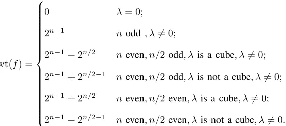
The weight of the Boolean function f :F2n→F2 defined as
f(a) = Trn(λa3) (31)
wt(f) =
0 λ= 0;
2n−1 nodd , λ6= 0;
2n−1−2n/2 neven, n/2odd, λis a cube, λ6= 0;
2n−1+ 2n/2−1 neven, n/2odd, λis not a cube, λ6= 0;
2n−1+ 2n/2 neven, n/2even, λis a cube, λ6= 0;
2n−1−2n/2−1 neven, n/2even, λis not a cube, λ6= 0.
(32)
Note that in the case ofa6= 0we can express the weight of has
wt(h) = 2n−wt(f)−1 (33)
forf(a) = Trn(λa3)withλ= (b+β3); we have to subtract1in the expression above in order to account for the
casea= 0. We can thus derive the following explicit formula for the value of|ΠβF(b)|.
Proposition 6. LetF(x) =x3 be over
F2n and letb, β∈F2n be arbitrary. Then
|ΠβF(b)|=
2n b=β3;
2n−1−1 b6=β3, nodd;
2n−1+ 2n/2−1 b6=β3, b+β3is a cube, neven, n/2 odd;
2n−1−2n/2−1−1 b6=β3, b+β3is not a cube, neven, n/2odd;
2n−1+ 2n/2−1−1 b=6 β3, b+β3is a cube, neven, n/2 even;
2n−1−2n/2−1 b=6 β3, b+β3is not a cube, neven, n/2even.
(34)
The value minb∈F2n|Π β
F(b)|is then equal to
min
b∈F2n
ΠβF =
2n−1−1 nis odd;
2n−1−2n/2−1−1 nis even, n/2is odd;
2n−1−2n/2−1 nis even, n/2is even
(35)
and the lower bound on the distance to the closest APN functionGcan be explicitly written as
d(F, G)≥
2n−1+2
3 nis odd;
2n−1−2n/2−1+2
3 nis even, n/2 is odd;
2n−1−2n/2+2
3 nis even, n/2 is even.
(36)
From this we can easily see that the distanced(F, G)tends to infinity withn. Observe that the value ΠβF does
not actually depend on the shift β; this is true for all quadratic functions as per Proposition 5.
Table I gives the values ofmF (forF(x) =x3) and the lower bound on the distance betweenx3 and the nearest
APN function for all dimensions n in the range 1 ≤ n ≤ 20. Note that for 1 ≤ n ≤ 4 the bound is tight as
• u1= 0,v1= 1for n= 1;
• u1= 0,v1=αfor n= 2, where αis a primitive element of F22;
• u1= 0,u2= 1,v1= 1,v2=αfor n= 3, where αis a primitive element of F23;
• u1= 0,u2= 1,v1= 1,v2= 1for n= 4.
In the case ofn= 5, we have experimentally verified that the smallest distance to an APN function is equal to
8, which shows that the lower bound is not tight. It is worth noting, furthermore, that in this case all possible APN
functions at distance 8 fromx3 were obtained by shifting 8 points from
F2n by the same valuev∈F2n.
TABLE I
VALUES OFmFAND LOWER BOUNDS ONd(F, G)FOR ANYGAPNFORF(x) =x3OVER
F2n
Dimension mx3 Lower bound on minimum distance
1 0 1
2 0 1
3 3 2
4 3 2
5 15 6
6 27 10
7 63 22
8 111 38
9 255 86
10 495 166 11 1023 342 12 1983 662 13 4095 1366 14 8127 2710 15 16383 5462 16 32511 10838 17 65535 21846 18 130815 43606 19 262143 87382 20 523263 174422
1) Minimum distance between APN functions: By Proposition 3, we know that the value mF for some given
APN function F and the lower bound K on the distance to the closest APN function derived from it are valid
not only for F itself, but for all functions belonging to its CCZ-equivalence class. Since all APN functions of
dimensions four and five have been classified up to CCZ-equivalence [3], Corollary 2 can now be used to obtain a
lower bound on the Hamming distance between any two APN functions overF2n withn∈ {4,5}by examining a
single representative from each. For higher dimensions, we can compute the lower bound for some of the known
CCZ-classes; since the problem of classifying all APN functions in those cases is still open, however, this gives
only a partial result.
Table II gives the values ofmFfor representatives from all switching classes [13] for dimensionn∈ {4,5,6,7,8}.
corresponding dimension. In the case ofn∈ {6,8}, the functions from are given and indexed according to Table
5 from [13]. For n= 7, we obtain the same bound for all functions listed in [13].
The last column of the table gives the minimum distance from a given functionF to the nearest APN function;
this can be computed simply asdmF/3e+ 1but is explicitly given here for convenience.
V. SINGLE SHIFT
A significantly simplified construction involves shifting all the pointsu1, u2, . . . , uK by the same valuev∈F∗2n.
In this case, characterizing the APN-ness of
G(x) =F(x) +v
X
i∈[K]
1ui(x)
becomes quite easy regardless of whetherF is assumed to be APN or not.
For a given triple(a, x, y)∈F32n, let us denote byNa,x,y the parity of the number of elements from{x, y, a+
x, a+y} that are inU, i.e.
Na,x,y=|{x, y, a+x, a+y} ∩U| mod 2.
Observe that some differential equation of the formDaG(x) =bfor givena∈F∗2n, b∈F2n can have more than
two solutions if and only if
DaF(x) +DaF(y) =vNa,x,y
for x, y∈F2n withx+y6=a.
Given some initial functionF overF2n, the following procedure can then be used to find all APN functionsG
that can be obtained fromF by shifting some set of pointsU by a given shift v∈F∗2n:
1) assign a Boolean variableux∈F2 to every field element x∈F2n; the value ofuxwill indicate whetherxis
in U or not;
2) find all tuples(x, y, a)∈F32n for which DaF(x) +DaF(y) =v witha6= 0, x6=y, a+y;
3) for every such tuple, consider the equationux+uy+ua+x+ua+y = 0;
4) find also all tuples(x, y, a)∈F3
2n for whichDaF(x) +DaF(y) = 0witha6= 0, x6=y, a+y; 5) for every such tuple, consider the equationux+uy+ua+x+ua+y = 1;
6) solve the system of all such equations; this can be done by e.g. constructing ane×(2n)matrix over
F2, where
eis the number of tuples of both types considered above;
7) the solutions to this system now correspond to precisely those sets U ⊆F2n for whichGis APN.
Note that in the case that F is APN, no equations of the type DaF(x) +DaF(y) = 0exist for x+y 6=a so
that steps four and five above can be skipped.
This method is quite useful in practice, as it can be applied rather efficiently (the main part of the computations
consists of finding all tuples(x, y, a) satisfying one of the conditions given above) and since it can be applied to
an arbitrary function F (not only APN). Note that the same method can be obtained from Theorem 9 in [13] for
TABLE II
VALUES OFmFAND LOWER BOUNDS ONd(F, G)FOR ANYG6=FAPNFORF(x)FROM[13]
Dimension F mF Distance 4 x3 3 2
5 x3 15 6
5 x5 15 6
5 x15 9 4
VI. CONCLUSION
We examined a construction in which a given vectorial Boolean function F is modified at K different points
in order to obtain a new function G. We obtained sufficient and necessary conditions for G to be APN, from
which we derived an efficient procedure for searching for APN functions at a given distance from F as well as a
lower bound on the distance to the closest APN function in terms of the quantitymF. Some properties concerning
the computation and invariance of mF were shown, and its values were experimentally computed for all known
switching classes [13], suggesting that this value grows proportionally with the dimension of the underlying finite
field. An additional method for characterizing the APN-ness ofGwas given for the special case when all the shifts
v1, v2, . . . , vK are identical.
There is lot of room for future work, and a number of questions and research directions remain open. The
methods used here for the characterizations of APN functions may be applied to other classes such as differentially
4-uniform functions. A theoretical lower bound on the value mF would be valuable, as well as additional results
related to its computation. Finding relations between mF and other properties of F may be very important, and
applying the filtering procedure in practice may lead to new examples of APN functions.
ACKNOWLEDGEMENTS
We would like to thank Nian Li for his support and advice and for his contribution to our research.
REFERENCES
[1] Thierry P. Berger, Anne Canteaut, Pascale Charpin, and Yann Laigle-Chapuy. On Almost Perfect Nonlinear Functions OverFn2. IEEE
Transactions on Information Theory, 52(9):4160–4170, 2006.
[2] Eli Biham and Adi Shamir. Differential Cryptanalysis of DES-like Cryptosystems.Journal of Cryptology, 4(1):3–72, Jan 1991. [3] Marcus Brinkmann and Gregor Leander. On the Classification of APN Functions up to Dimension Five.Designs, Codes and Cryptography,
49:273–288, 2008.
[4] Lilya Budaghyan. The Equivalence of Almost Bent and Almost Perfect Nonlinear Functions and Their Generalizations. PhD thesis, Otto-von-Guericke-University Magdeburg, 2005.
[5] Lilya Budaghyan, Claude Carlet, Tor Helleseth, Nian Li, and Bo Sun. On Upper Bounds for Algebraic Degrees of APN Functions.IEEE
Transactions on Information Theory, 64(6):4399–4411, 2018.
[6] Lilya Budaghyan, Claude Carlet, and Gregor Leander. Constructing New APN Functions from Known Ones. Finite Fields and Their
Applications, 15(2):150–159, 2009.
[7] Lilya Budaghyan, Claude Carlet, and Alexander Pott. New Classes of Almost Bent and Almost Perfect Nonlinear Polynomials. IEEE
Transactions on Information Theory, 52(3):1141–1152, 2006.
[8] Claude Carlet. Vectorial Boolean Functions for Cryptography. Boolean models and methods in mathematics, computer science, and
engineering, 134:398–469, 2010.
[9] Claude Carlet. Boolean and Vectorial Plateaued Functions and APN Functions.IEEE Transactions on Information Theory, 61(11):6272– 6289, 2015.
[10] Claude Carlet, Pascale Charpin, and Victor A. Zinoviev. Codes, Bent Functions and Permutations Suitable for DES-like Cryptosystems.
Designs, Codes and Cryptography, 15(2):125–156, 1998.
[11] Leonard Carlitz. Explicit Evaluation of Certain Exponential Sums. Mathematica Scandinavica, 44:5–16, 1979.
[12] Florent Chabaud and Serge Vaudenay. Links between Differential and Linear Cryptanalysis. InWorkshop on the Theory and Application
of Cryptographic Techniques, EUROCRYPT 94, volume 950, pages 356–365, 1994.
[13] Yves Edel and Alexander Pott. A New Almost Perfect Nonlinear Function which is not Quadratic. Advances in Mathematics of
[14] Nikolay Kaleyski. Changing apn functions at two points.Cryptography and Communications.
[15] Philippe Langevin. Covering Radius ofRM(1,9)inRM(3,9).EUROCODE ’90, Proceedings of the International Symposium on Coding
Theory and Applications, pages 51–59, 1990.
[16] Kaisa Nyberg. Differentially Uniform Mappings for Cryptography.Lecture Notes in Computer Science, 765:55–64, 1994.
[17] Kaisa Nyberg. S-boxes and round functions with controllable linearity and differential uniformity. InInternational Workshop on Fast
Software Encryption, pages 111–130, 1994.
[18] Lawrence C. Washington and Wade Trappe.Introduction to Cryptography with Coding Theory. Prentice Hall, 2002.
[19] Yuyin Yu, Mingsheng Wang, and Yongqiang Li. Constructing differentially 4 uniform permutations from known ones. Chinese Journal
of Electronics, 22(3):495–499, 2013.
[20] Yuliang Zheng and Xian-Mo Zhang. Plateaued Functions. InICICS ’99 Proceedings of the Second International Conference on Information