Western University Western University
Scholarship@Western
Scholarship@Western
Electronic Thesis and Dissertation Repository
9-26-2014 12:00 AM
Energy Based Multi-Model Fitting and Matching Problems
Energy Based Multi-Model Fitting and Matching Problems
Hossam N. Isack
The University of Western Ontario
Supervisor Yuri Boykov
The University of Western Ontario Graduate Program in Computer Science
A thesis submitted in partial fulfillment of the requirements for the degree in Doctor of Philosophy
© Hossam N. Isack 2014
Follow this and additional works at: https://ir.lib.uwo.ca/etd
Part of the Artificial Intelligence and Robotics Commons, Other Computer Sciences Commons, and the Theory and Algorithms Commons
Recommended Citation Recommended Citation
Isack, Hossam N., "Energy Based Multi-Model Fitting and Matching Problems" (2014). Electronic Thesis and Dissertation Repository. 2426.
https://ir.lib.uwo.ca/etd/2426
This Dissertation/Thesis is brought to you for free and open access by Scholarship@Western. It has been accepted for inclusion in Electronic Thesis and Dissertation Repository by an authorized administrator of
(Thesis format: Integrated Article)
by
Hossam Isack
Graduate Program in Computer Science
A thesis submitted in partial fulfillment
of the requirements for the degree of
Doctor of Philosophy
The School of Graduate and Postdoctoral Studies
The University of Western Ontario
London, Ontario, Canada
c
Abstract
Feature matching and model fitting are fundamental problems in multi-view geometry. They are chicken-&-egg problems: if models are known it is easier to find matches and vice versa. Standard multi-view geometry techniques sequentially solve feature matching and model fitting as two independent problems after making fairly restrictive assumptions. For example, matching methods rely on strong discriminative power of feature descrip-tors, which fail for stereo images with repetitive textures or wide baseline. Also, model fitting methods assume given feature matches, which are not known a priori. Moreover, when data supports multiple models the fitting problem becomes challenging even with known matches and current methods commonly use heuristics.
One of the main contributions of this thesis is a joint formulation of fitting and matching problems. We are first to introduce an objective function combining both matching and multi-model estimation. We also propose an approximation algorithm for the corresponding NP-hard optimization problem using block-coordinate descent with respect to matching and model fitting variables. For fixed models, our method uses min-cost-max-flow based algorithm to solve a generalization of a linear assignment problem with label cost (sparsity constraint). The fixed matching case reduces to the multi-model fitting subproblem, which is interesting in its own right. In contrast to standard heuristic approaches, we introduce global objective functions for multi-model fitting using various forms of regularization (spatial smoothness and sparsity) and propose a graph-cut based optimization algorithm, PEaRL. Experimental results show that our
proposed mathematical formulations and optimization algorithms improve the accuracy and robustness of model estimation over the state-of-the-art in computer vision.
Keywords: Multi-view Geometry, Fitting, Matching, Flow recycling, Label Cost.
Chapter 1 is my work to summarize fitting, matching and multi-labeling problems.
Chapters 2 and 4 were a collaborative effort with my advisor, Yuri Boykov.
Chapter 3 was a close collaboration with Andrew Delong, Anton Osokin, and Yuri Boykov. My contributions were the global energy formulation and all the necessary model fitting experiments. Andrew Delong proposed the main technical idea on how to extend
α-expansion to handle label costs.
Dedication
To my loving parents, thank you for your help. I miss being with you every day.
To my lovely fianc´e, thank you for your support. I promise I will always be there for you.
Abstract ii
Co-Authorship Statement iii
List of Figures vii
List of Tables xiii
1 Introduction 1
1.1 Multi-view Geometry Overview . . . 1
1.1.1 Thin Lens Model . . . 1
1.1.2 Pinhole Camera Model . . . 2
1.1.3 Stereo Vision . . . 5
Plane Induced Homography . . . 5
Fundamental Matrix . . . 6
1.2 Multi-Labeling Problem Overview . . . 8
1.3 Thesis Overview . . . 12
1.3.1 Basic Problem Formulation . . . 12
1.3.2 Summary of Contributions . . . 13
1.3.3 Thesis Structure . . . 16
2 Energy-based Geometric Multi-Model Fitting 19 2.1 Introduction . . . 20
2.1.1 Towards Energy Optimization . . . 21
2.1.2 Related Work . . . 26
2.2 Our Approach (PEaRL) . . . 28
2.2.1 Proposing Initial Labels . . . 28
2.2.2 Energy Formulation . . . 29
2.2.3 Outliers . . . 30
2.2.4 Expand and Re-estimateLabels . . . 31
2.2.5 Algorithm and Its Properties . . . 32
2.3 Experimental Results . . . 39
2.3.1 Estimating Multiple Affine Models . . . 40
2.3.2 Estimating Multiple Homographies . . . 43
2.3.3 Motion Segmentation . . . 48
Using two-views . . . 48
Using multiple views/frames . . . 53
2.4 Conclusions . . . 55
3 Fast Approximate Energy Minimization with Label Costs 60 3.1 Some Useful Regularization Energies . . . 60
3.2 Fast Algorithms to Minimize (?) . . . 65
3.2.1 Expansion moves with label costs . . . 65
3.2.2 Optimality guarantees . . . 67
3.2.3 Easy case: only per-label costs . . . 69
3.2.4 Energy (?) as an information criterion . . . 70
3.3 Working With a Continuum of Labels . . . 70
3.4 Applications and Experimental Setup . . . 73
3.4.1 Geometric multi-model fitting . . . 75
3.4.2 Image segmentation by MDL criterion . . . 77
3.5 Discussion . . . 77
4 Energy based multi-model fitting & matching for 3D reconstruction 80 4.1 Introduction . . . 80
4.2 Fit-&-Match Energy . . . 82
4.3 Overview of Our Approach . . . 83
4.4 Optimization . . . 84
4.4.1 Solving GAP . . . 85
Reducing GAP to LAP . . . 85
LAP as MCMF (overview) . . . 85
Solving MCMF (overview) . . . 86
Solving a Series of GAPs . . . 86
4.4.2 Local Search-GAP (LS-GAP) . . . 86
4.5 Evaluation . . . 87
4.6 Conclusions . . . 93
5 Conclusion 94
Curriculum Vitae 95
1.1 (a) shows a thin lens model and (b) shows its basic functional properties. 2
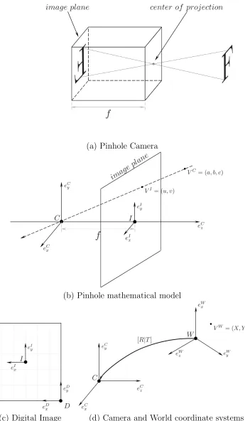
1.2 (a) shows a pinhole camera model and (b) shows the pinhole mathematical model with an “imaginary” image plane in front of the center of projection, also the camera coordinate system C is located a the center of projection. (c) shows the image plane coordinate system I relative to the digital image coordinate systemD. (d) shows a rigid transformation [R|T] tying the camera coordinate systemC and the world coordinate system W. . . 3
1.3 (a) and (b) show plane projection in single and stereo camera settings, respectively. . . 6
1.4 (a) Stereo images showing epipoles and epipolar line corresponding to x. Figure (b) shows how knowing matches in a stereo setting allows us to recover 3D information of scene points. . . 8
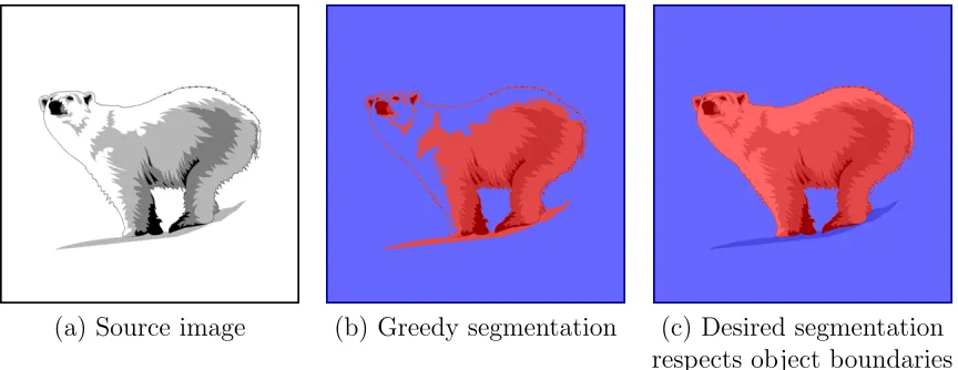
1.5 (a) is the image to be segmented. (b) and (c) show segmentation results where the foreground is red shaded and the background is blue shaded. Labeling the white part of the polar bear using only color cue is not suffi-cient as it is equally likely to be foreground or background. When labeling variations is discouraged as in (c) labeling the white part of the polar bear as a foreground becomes a more favorable solution. . . 9
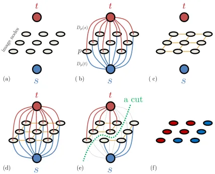
1.6 (a) graph nodes. Figures (b) and (c) show the edges corresponding to the unary and pairwise potentials of equation (1.20), respectively. The constructed graph G is shown in (d). Figure (e) shows a possible s\t-cut and (f) shows its corresponding pixel labeling. In (e) the severed edges by the s\t-cut are shown in gray color. . . 10 1.7 (a) shows a pair of images with parts (green and blue) that undergo
differ-ent translations. (b) shows feature sets Fl and Fr, and a possible match.
(c) shows translations θi and θj that the green and blue parts undergo.
(d) shows an ideal labeling: green’s part features (inside green cloud) are labeled i and blue’s part features (inside blue cloud) are labeledj. . . 14
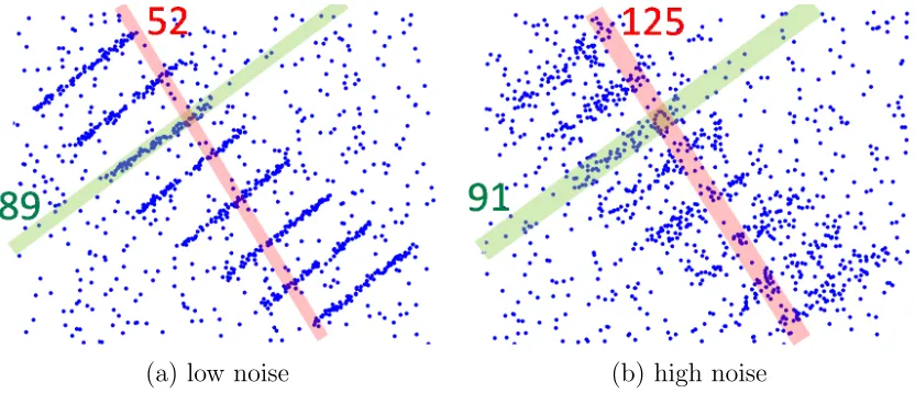
2.1 Blue dots are data points supporting 8 lines. In multi-model cases, detect-ing models by maximizdetect-ing the number of inliers may work for low levels of noise (a). Higher noise levels require larger thresholds to detect inliers (b), but then some random model (red) may have far more inliers than the true model (green). The integers show the number of model inliers for the selected thresholds. Simplistic greedy selection of models with the largest number of inliers would fail in (b). This example illustrates a general prob-lem that affects many multi-model fitting approaches that greedily selects one model at a time while ignoring the overall solution. It also motivates our global energy approach that considers the quality of the whole solution. 20 2.2 Motivating spatial regularization in geometric model fitting. In many
vi-sion problems combining geometric errors and spatial coherence terms in energy (2.3) can be justified generatively because clusters of inliers are generated by regular objects (a). Moreover, spatial regularization can also be justified discriminatively. Plot (b) shows an average deviation from the ground truth for optimal models obtained in 100 randomly generated line-fitting tests as in Fig. 2.4(d). Each point in this plot corresponds to some fixed smoothness parameterλin (2.3). Clearly, the spatial coherence term significantly reduces estimation errors for someλ >0 . . . 21 2.3 Examples of inlier classification from thresholding. If data is known to
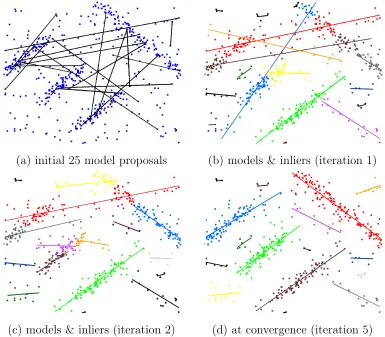
support one model (a) then thresholding identifies inliers (blue) for any model without ambiguity. In case of 3 models (b), simple thresholding may not disambiguate inliers (red) between the models. . . 23 2.4 Illustration of PEaRL’s iterations. (a) proposals generated by random
sampling, (b-d) re-estimation of models and their inliers after several iter-ations ofexpandand re-estimatesteps for energy (2.3) or (2.7). Note that the algorithm may converge to good models even from a small set of rough guesses. In this example we did not use anoutlier label, see Section 2.2.3, and an optimal set of lines in (d) “explains” all data points. . . 29 2.5 We use Delaunay triangulations of data points. K-nearest points or other
techniques can be used as well, particularly for higher dimensional data. We did not observe much difference in practical performance. . . 31
2.6 PEaRL vs RANSAC for synthetic data sets with 80% uniformly
dis-tributed outliers and 20% noisy inliers supporting one line model. In each test both methods used the same initial set of randomly sampled model proposals. X-axis is the number of initially proposed models. Y-axis shows estimation errors w.r.t. the parameters of the ground truth line model. The errors are averaged over 400 randomly generated tests.
RANSAC basically selects the best model from the initial set of
propos-als. By iteratively minimizing global energy (2.3) PEaRL can converge
to a much better model than those in the initial set. In contrast, stan-dardRANSACstrongly relies on a larger number of initial samples to find
accurate estimates. . . 34
200 random outliers were added. Outliers represent 25% of the data. . . . 35 2.8 Comparing the results for fitting lines to noisy data points. The data
points were perturbed with medium Gaussian noise ( σ = 0.02) and in-cluded 300 random outliers. Outliers represent 35% of the data. . . 36 2.9 Comparing the results for fitting lines to noisy data points. The data
points were perturbed with high Gaussian noise ( σ = 0.025) and 500 random outliers were added. Outliers represent 45% of the data. . . 37 2.10 Intersecting lines example. Optimization of energy (2.3) may leave
spa-tially isolated groups of inliers assigned to 2 models even if their parame-ters are infinitesimally close (b). Per-label costs in energy (2.7) solves this problem (c) but requires either an additional merging operation or an ex-tension ofα-expansion—introduced in Chapter 3. This example motivates the use of the EM-style soft assignments of labels to points. However, in computer vision as will be shown in Sec. 2.3 we get occlusions (not inter-sections), which better motivates our “hard” assignments of labels. . . . 38 2.11 Fitting lines with different noise levels. The inliers in (a) were generated
with different levels of Gaussian noise. 40% of the data are outliers. In (b) PEaRLestimated labels combining geometric model parameters with
unknown noise variances using error measure (2.8). Previous multi-model fitting methods use fixed thresholds to identify inliers, which would not work in this case. . . 39 2.12 Geometric fitting errors ||p−A|| for rectified stereo. Assuming matched
points p = {pl, pr} are on the corresponding epipolar (scan) lines ∆y =
yl − yr = 0, the left transfer error is a horizontal shift ∆x between pr
and Apl as shown in (a). The standardre-projection error (b) is obtained
by treating points pl and pr as noisy observations of some hidden “true”
pair of matched points ¯p ={p¯l,p¯r} where ¯pr = Ap¯l and ¯p minimizes the
observation noise min|p¯l−pl|2+|p¯r−pr|2. . . 41
2.13 Results for ”Clorox” stereo pair [2]. (a) Dense pixel segmentation by BT [2] uses photo-consistency. (b-c) Sparse inlier classification by PEaRL
using geometric fit measures (2.9) and (2.10), respectively. . . 43 2.14 Comparison of results by BT [2] and PEaRL. Lines are computed for all
pairs of intersecting planes (affine models). . . 44 2.15 Typical results for affine model fitting in Sec. 2.3.1 via sequentialRANSAC
(a) and J-linkage [26]. We used 5000 uniform samples for RANSAC. Differ-ent threshold values did not give much improvemDiffer-ent. Similarly, differDiffer-ent tunings of J-linkage generated various artifacts. These problems might be explained by the large level of noise in the data, as in Fig. 2.9. . . 44 2.16 Multi-homography fitting, images from VGG (Oxford) Merton College I. 45 2.17 Multi-homography fitting for stereo images from VGG (Oxford) Merton
College III. Both results were obtained using standard SIFT features. . . 46
2.18 Multi-homography fitting for “stairs” stereo image from VGG (Oxford). The results in (b) and (c) represent our best efforts in tuning RANSAC
and J-linkage thresholds. For example, two “walls” start to grab false positive matches for larger threshold values, while for smaller thresholds the “stairs” become even more over-segmented compared to what is shown here. . . 46
2.19 In this Raglan Castle example from VGG (Oxford) we used the same color more than once to represent different planes (a). Only spatially connected planes are shown in different colors. An image of the same scene from a different view (b) confirms that the vertical walls of the building corresponds to different planes. . . 47
2.20 Representative PEaRL’s results for motion sequences from Rene Vidal’s
data set [31]. Our motion estimation using mixtures of fundamental ma-trices (Sec. 2.3.3) uses only two frames (the first and the last). . . 50
2.21 Optimal solution for energy (2.3). In contrast to results for energy (2.7) in Fig.2.20 (e)-(h), it fails to generate one background motion from yellow, green, and red clusters. These clusters correspond to infinitesimally close motions, but they are spatially isolated. The third term in (2.7) addresses this issue. . . 51
2.22 Histogram of misclassification errors for PEaRL with energy (2.13) on 26
Checkerboard examples [31] with 3 distinct motions. This histogram re-veals two “modes”. The mode with smaller misclassification errors mainly contains examples wherePEaRLproduced exactly 3 models. Such
exam-ples are marked in blue. Examexam-ples where PEaRL produced a different
number of models are marked in red. Such examples formed the “gross errors” mode. The percentage of misclassified points may not be a proper measure for comparing a method that automatically computes the number of models against the methods thata prioriknow the correct number. We separately reportPEaRL’s error statistics for 15 (blue) examples with the
correct number of obtained models, see ER1in Table 2.2. . . 51
2.23 Scatter plot of different solutions obtained by PEaRLon one of the
exam-ples in [31] using different sets of 5000 (uniformly) sampled fundamental matrices. This number of samples is statistically insufficient for the motion estimation examples in Sec. 2.3.3 (see text) and the quality of optimiza-tion may suffer. The plot also illustrates positive correlaoptimiza-tion between the values of our energy (2.13) and the misclassification errors. . . 52
2.24 Representative PEaRL’s results using energy (2.15) for motion sequences
from Vidal’s data set [31]. Unlike the fundamental matrix fitting method in Sec. 2.3.3, this formulation uses all frames in the sequence. . . 54
2.25 Multi-motion estimation accuracy in one of the checkerboard sequences from Sec. 2.3.3. Misclassification errors are shown for optimal solutions corresponding to different values ofλ and β in energy (2.15). . . 55
gives coherent segmentations (c) but finds redundant motions. Our energy (?) combines the best of both (d). . . 61 3.2 Planar homography detection on VGG (Oxford) Merton College 1
im-age (right view). Energy (3.1) finds reasonable parameters for only the strongest 3 models shown in (b), and still assigns a few incorret labels. Energy (3.2) finds reasonable clusters (c) but fits 9 models, some of which are redundant (nearly co-planar). Our energy (?) finds both good param-eters and labels (d) for 7 models. . . 63 3.3 Unsupervised segmentation using histogram models. Energy (3.1) clusters
in colour space, so segments (b) are incoherent. Energy (3.2) clusters over pixels and must either over-segment or over-smooth (c), just as in [26]. Our energy (?) balances these criteria (d) and corresponds to Zhu & Yuille [27] for segmentation. . . 64 3.4 Left: Graph construction that encodes h−hx1x2· · ·xk when we define
xp = 1⇔p∈T whereT is the sink side of the cut. Right: In a minimum
s-tcut, the subgraph contributes cost either 0 (allxp = 1) orh(otherwise).
A cost greater than h (e.g. ∗) cannot be minimal because setting y = 0 cuts only one arc. . . 66 3.5 Re-estimation helps to align models over time. Above shows 900 raw data
points with 50% generated from 5 line intervals. Random sampling proposes a list of candidate lines (we show 20 out of 100). The 1st segmentation and re-estimation corresponds to Li [18], but only the yellow line and gray line were correctly aligned. The decreasing energies in Figure 3.8 correspond to better alignments like the subsequent iterations above. If a model loses enough inliers during this process, it is dropped due to label cost (dark blue line). . . 71 3.6 We can also fit line intervals to the raw data in Figure 3.5. The three
results above were each computed from a different set L of random initial proposals. See Section 3.4.1 for details. . . 73 3.7 For multi-model fitting, each label can represent a specific model from any
family (Gaussians, lines, circles...). Above shows circle-fitting by minimiz-ing geometric error of points. . . 73 3.8 Energy (?0) over time for a line-fitting example (1000 points, 40% outliers, 6
ground truth models). Only label cost regularization was used. Re-estimation reduces energy faster and from fewer samples. The first point (•) in each series is taken after exactly one segmentation/re-estimation, and thus suggests the quality of Li [18] using a greedy algorithm instead of LP relaxation.. . . 74 3.9 Unsupervised segmentation by clustering simultaneously over pixels and colour
space using Gaussian mixtures (colour images) and non-parametric histograms (greyscale images). Notice we find coarser clustering on baseball than Zabih & Kol-mogorov [26] without over-smoothing. For segmentation, our energy is closer to Zhu & Yuille [27] but our algorithm is more powerful than region-competition. 76
4.1 Best seen in Color, Fig. (a) shows the effect of EFM iterations on energy (4.1). EFM converged on the average after 5 iterations, and each iteration on the average took 1 min. Figure (b) shows multiple histograms of the final energies for different sizes of initial set of proposals—blue indicates a large set of proposals. The larger the set of initial proposals L the more likely that EFM will converge to a low energy. . . 89 4.2 Best seen in Color, Fig. shows ROC curve for standard SIFT matches by
varying SBR threshold, and the scatter plot represents EFM results for different sizes of initial set or proposals. As can be seen, the lower the final energy (blue) the better the matching. . . 90 4.3 Best seen in Color, Fig. (a) shows EFlabeling result (average TPR=0.51
and FPR=1.6E-05) and (b) shows EFMlabelingresult (average TPR=0.98 and FPR=9.1E-06). Features assigned to the same model/label are drawn in the same color and unmatched features are shown as white x. Figures (c-f) show the enlargement of segments 1 and 2 in (a) and (b). Figures (g-h) show the matching, between two small regions in the stereo images, of the EF and EFM results, respectively. . . 91 4.4 Best in Color, the first column shows one of the stereo images for each
example, second and third columns show the EF and EFMlabellingresults superimposed on the images shown in the first column, respectively. On average of 50 runs, EFM found 0.75, 10.53, 3.31, 0.44, and 0.68 times more inliers than EF. EFM and EF+GM results where comparable, EFM found approximately between 0.05 and 0.08 times more matches. . . 92
2.1 Geometric errors for lines in Fig. 2.14 where affine models intersect. Er-rors are computed as the sum of distances between the ground truth line segment corners and the computed lines. The errors for sequential
RANSACand J-linkage, see Fig. 2.15, were significantly larger than those
above. . . 43 2.2 Misclassification errors for checkerboard motion estimation sequences in
[31]. The results for REF, GPCA [32], LSA [36], and RANSAC are
copied from Table 4 in [31]. These methods use all N-frames in each video sequence. In contrast, our results for PEaRL with energy (2.13)
use only 2 frames, the first and the last in the sequence. Other methods also “know” that the exact number of models is 3. In contrast, PEaRL
may obtain a different number of models. Figure 2.22 illustrates how this affects PEaRL’s classification errors. For a more balanced comparison we
show 2 additional statistics. First, column ER1 evaluates 15 out of 26
examples where PEaRL obtained exactly 3 models. Second, similarly to
REF [31], column ER2 evaluates the “reference” solutions obtained by
PEaRLfrom the ground truth models in all 26 examples. . . 49
2.3 Misclassification errors for checkerboard motion estimation sequences in [31]. The results for REF, GPCA [32], LSA [36], and RANSAC are
copied from Table 4 in [31]. All methods in this table use all frames in each video sequence. PEaRL may obtain a different number of models
while the other methods “know” that the exact number of models is 3. For a more balanced comparison we show 2 additional statistics. First, column
ER1 evaluates 12 out of 26 examples where PEaRL obtained exactly 3
models. Second, similarly to REF in [31], column ER2 evaluates the
“reference” solutions obtained by PEaRL from the ground truth models
in all 26 examples. . . 56
4.1 Graphite VGG Oxford dataset, single model and increasing baseline. The table shows the averages of GQ and ROC attributes, over 50 runs, for EFM, EF, and EF+GM model estimates. . . 90
Chapter 1
Introduction
Sections 1.1 and 1.2 are intended for readers who are not familiar with multi-view ge-ometry, and common multi-labeling problems in computer vision and their optimization frameworks. In Section 1.1, we will overview some basic multi-view geometry principles [10, 7] e.g. camera models and stereo vision. Then, in Section 1.2, we will discuss a com-mon multi-labeling problem and give a brief overview of the α-expansion algorithm [4] which is widely used in computer vision for multi-labeling problems. Finally, in Section 1.3 we overview the problems we are trying to solve and summarize our contributions.
1.1
Multi-view Geometry Overview
We will start by studying some basic camera models, i.e. thin lens and pinhole camera. Then we will discuss plane induced Homographies and the fundamental matrix which could be used to detect planes and rigid motions in a scene, respectively.
1.1.1
Thin Lens Model
For simplicity, the following discussion is limited to converging thin lens. In a nutshell, a thin lens has a negligible thickness, i.e. the distance between the two surfaces of the lens, compared to the radii of curvature of the lens’ surfaces. Let us denote the optical center of the lens by C see Fig. 1.1(a). Also, let the optical axis be the line perpendicular to the lens and passing through C. The focal length f is the main parameter of any lens. Knowing the focal length of a converging thin lens allows us to identify two focal points on each side of the lens, and each focal point is along the optical axis and at a distance
f from C. The functional properties of a thin lens, as shown in Fig. 1.1(b), are:
• The direction of any ray entering the lens through the optical center will not be affected.
• Any ray entering the lens parallel to the lens’s optical axis on one side will be refracted on the other side to intersect the optical axis at a distance f from the optical center.
• Any ray that enters the lens after passing through the focal point from one side will come out parallel to the optical axis on the other side.
(a) Thin lens (b) Functional properties
Figure 1.1: (a) shows a thin lens model and (b) shows its basic functional properties.
Another parameter is the aperture opening/hole of diameter D which restricts the range of rays passing through or reaching the lens, as the aperture opening could be located on either side of the lens, see Fig. 1.1(a). An ideal thin lens model has an infinitesimal aperture which in theory only allows rays that are going through the optical center resulting in a purely refractive lens [14]. This idealization is also known as pinhole camera model.
1.1.2
Pinhole Camera Model
The pinhole camera model is one of the simplest and oldest camera models, Fig. 1.2(a). Other camera models e.g. affine camera models, orthographic projection model etc. are discussed in [10]. A full and comprehensive discussion on camera models is beyond the scope of this work. In this work we discuss the pinhole model since it is considered a good geometric approximation of the ideal thin lens—with infinitesimally small aperture. As can be seen in Fig. 1.2(a) the formed image is always flipped horizontally and vertically on the image plane. In our pinhole mathematical model we adopt the frontal image plane approach where an imaginary plane is placed in front of the center of projec-tion. To describe the mathematical model we first need to define two coordinate systems:
camera coordinate system C with the basis {eCx, eCy, eCz} and the image plane coordinate system I with the basis {eI
x, eIy}, see Fig. 1.2(b). Also, the image plane is placed at a
distance f fromC and with a normaleC
z. Later on we will define other coordinate
sys-tems and, to avoid any ambiguity, the superscript of a vector in our notation will denote which coordinate system the vector is defined with respect to, e.g. eC
x is a vector defined
with respect to C.
LetVC = [a, b, c]T be a point on the imaged object andVI = [u, v]T be its projection on the image plane. Knowing that the image plane is atf with normaleC
z, by projecting
VC on{eC
x, eCz} and {eCy, eCz}, and using triangle similarities we can deduce that
u=fa
c (1.1)
v =fb
1.1. Multi-view Geometry Overview 3
(a) Pinhole Camera
(b) Pinhole mathematical model
(c) Digital Image (d) Camera and World coordinate systems
To avoid the nonlinearity in relating VI and VC in equations (1.1) and (1.2), we
will use homogeneous coordinates to represent VI instead of Euclidean coordinates. Let
X = [x1, x2, . . . xn]T be a point inRn. To represent this point in homogeneous coordinates
we add a coordinate and set it to 1, X = [x1, x2, . . . xn,1]T. In our notation X is the
homogeneous representation ofX. In Projective coordinate systems where homogeneous coordinates are used scaling is not important
[x1, x2, . . . , xn,1]T '[λx1, λx2, . . . , λxn, λ]T
where A ' B means that there exists a scale c 6= 0 such that A = cB. By using the homogeneous coordinates of VI, we can linearly relateVI toVC
u v 1 '
f 0 0 0 f 0 0 0 1
a b c
. (1.3)
The digital image, is a discretized version of the image plane, see Fig. 1.2(c). In the digital image the origin is usually not in the middle of the image and the coordinates are in pixels not metric units like the image plane coordinates. Let the coordinate systemD
with the basis {eDx, eDy } be the digital image coordinate system and VD = [x, y]T be the transformed VI = [u, v] from the I coordinate system, see Fig. 1.2(c). Also, let m
u and
mv be the pixels/unit resolution of the digital image and [tu, tv] be the translation from
I toD. Now we can relateVD toVC as follows
x y 1 '
mu 0 0
0 mv 0
0 0 1
1 0 tu
0 1 tv
0 0 1
f 0 0 0 f 0 0 0 1
a b c '
muf 0 mutu
0 mvf mvtv
0 0 1
a b c
. (1.4)
In real life we never know the scene points coordinates with respect to the camera coordinate system C. However, it is possible to introduce a new coordinate system, namely world coordinate system W with the basis {eW
x , eWy , eWz }, to define the scene
points. The world coordinate system could be chosen arbitrarily, see Fig. 1.2(d). Also, let [R|T] be the 3D transformation that transforms W to C where R and T are the 3D rotation and translation, respectively. Let VW = [X, Y, Z]T be the scene point defined
with respect to W such that
VI = [R|T]VW. (1.5) Using (1.5) and (1.4) we can relate a world point VW to its pixel location VD on the
1.1. Multi-view Geometry Overview 5 x y 1 '
muf 0 mutu
0 mvf mvtv
0 0 1
[R|T] X Y Z 1 (1.6)
VD 'K[R|T]VW (1.7)
VD 'PVW. (1.8)
The upper triangular 3×3 matrixK in (1.7) is commonly referred to as the camera matrix and it contains all the intrinsic camera parameters, e.g. focal length and resolution. The R and T are extrinsic parameters, as they define the camera position relative to a world coordinate system of our choosing. Finally, the 3×4 matrix P in (1.8) denotes the projection matrix of a pinhole camera.
1.1.3
Stereo Vision
Capturing a scene from one viewpoint, i.e. a camera, is not enough to recover depth information to reconstruct the 3D scene—an image point could be the image of any 3D point a long the ray from the camera center of projection through that point. In stereo vision, two cameras are used to capture a scene from two different viewpoints. The stereo setting imitates human vision. Using a pair of stereo images one could recover depth information, i.e. reconstruct the scene. Also, planes in the scene could be detected by computing their plane induced homographies. There are different kinds of 3D recon-structions, e.g. projective, euclidian and metric reconstruction, see [10] for more details. In this work we will not discuss 3D reconstruction methods but rather an essential piece of information used in 3D reconstruction, i.e. the fundamental matrix.
Plane Induced Homography
A set of planar points and their projections onto a digital image could be related by a projective transformation, namely homography. In order to simply our derivation of the homography transformation, we will choose the world coordinate systemW such that its {ewx, ewy} basis span the 2D plane, see Fig. 1.3(a). Let VW = [X, Y, Z]T be a world point that belongs to the plane and VD = [x, y]T be its projection on to the digital image.
Note that any point that belongs to the plane will have Z = 0 by construction. From equation 1.6 we can deduce the following
x y 1 '
muf 0 mutu
0 mvf mvtv
0 0 1
r11 r12 r13 t1
r21 r22 r23 t2
r31 r32 r33 t3 X Y 0 1 (1.9) '
muf 0 mutu
0 mvf mvtv
0 0 1
r11 r12 t1
r21 r22 t2
r31 r32 t3
| {z }
Homography X Y 1
A homography in equation (1.10) is a 3×3 matrix. It should be noted that a general homography has 8 degrees of freedom not 9 since we could always set one of the 9 parameters to 1 to enforce equality in (1.10).
In the stereo setting shown in Fig. 1.3(b), let the two cameras’ center of projections be denoted by C1 and C2, respectively. Also, let the world plane be projected onto the two
images by the homographies H1 and H2. The projective transformation H that relates
the plane projections on these two images is also a homography
H =H2H
−1
1 .
In this example, H will transform the projected image of the plane from the first image to the second one.
(a) Single camera and projected plane (b) Stereo cameras and projected plane
Figure 1.3: (a) and (b) show plane projection in single and stereo camera settings, respectively.
Fundamental Matrix
Before we can define and derive the fundamental matrix we will cover some basic stereo vision concepts. As we mentioned earlier, depth information cannot be recovered using only one camera. Using only one camera, if x is the projection of a world point X then we can deduce that X lies on the ray from the camera center of projection to x, see Fig. 1.4(a) consider only the left camera. Now let us consider a stereo setting where the cameras’ relative orientation is known, as in Fig. 1.4(a). In that case we can easily deduce that the projection of X onto the second camera can only lie on the line of intersection between the camera’s image plane and the xCC0 plane, i.e the epipolar plane. We will refer to that line as the epipolar line corresponding to x, see Fig. 1.4(a). Also, we will refer to the points of intersection between the images’ planes and CC0 by epipoles e and
1.1. Multi-view Geometry Overview 7
position of the two cameras and their camera matrices, and this is why it is a vital part for 3D reconstruction.
The fundamental matrix F is a transformation. It transforms a point, e.g. x, from the left image to its corresponding epipolar line, i.e. line containinge0 andx0, in the right image, see Fig. 1.4(b),
Fx'e0 ×x0. (1.11) Recall thatxis the homogeneous coordinate representation ofx. In our derivation of the fundamental matrix, we will denote the projection matrices of the left and right images byP and P0, respectively. The epipole e0 is the projection of C onto the image plane of
C0
e0 'P0C. (1.12) Furthermore, let x be the projection of X on C, i.e. x ' P X. Let P+ be the pseudo
inverse of P and since P is a rectangular matrix with linearly independent rows then
P P+ = I. The world point P+x belongs to the line CX, i.e. its projection on C is x, since x'P P+x.
In addition, let ˆx0 be the projection ofP+xon C0 ˆ
x0 'P0P+x. (1.13) The point ˆx0 lies on the line e0x0 because the line CX is projected on toC0 over the line
e0x0. Therefore,
Fx'e0 ×xˆ0. (1.14) In equation (1.14) we could substitute e0 and ˆx0 from (1.12) and (1.13), respectively
Fx'(P0C)×(P0P+x). (1.15) Also,C andC0 are related by unknown [R|T] by construction. Now let us choose the world coordinate system to be C, i.e. C = 0 where 0 is the zero vector. Then we can deduce the following
P =K[I|0], (1.16)
P0 =K0[R|T], (1.17)
P+ =
K−1
0T
. (1.18)
Using (1.15) to (1.18), we can represent F in terms of the camera matrices and their relative position as follows
Fx'(P0C)×(P0P+x) '(K0T)×(K0RK−1x) '[K0T]×K0RK−1
| {z }
Fundamental matrix
(a) Stereo setting with unknown matches (b) Stereo setting with known matches Figure 1.4: (a) Stereo images showing epipoles and epipolar line corresponding to x. Fig-ure (b) shows how knowing matches in a stereo setting allows us to recover 3D information of scene points.
where [v]× denotes the skew symmetric matrix representation1 of vector v, e.g. let v =
[a, b, c]T then
[v]× =
0 −c b c 0 −a
−b a 0
.
The fundamental matrix could be used to track rigid motions in a scene [12]. Our derivation of the fundamental matrix came from a stereo setting where we used two cameras and the scene/object was static. Another way to arrive to the same conclusion is to use one none moving camera and take two pictures of a rigidly moving object/scene. In that case, theRandT in (1.19) will correspond to the rigid-body’s motion. Furthermore, if there is more than one object undergoing different rigid motions each of them will have it is own fundamental matrix. Thus, we can detect and identify multiple rigid motions in a scene by estimating multiple fundamental matrices.
1.2
Multi-Labeling Problem Overview
In computer vision many problems require assigning a label to every pixel, feature or substructure of an image. These labels could be color models, disparities, objects etc. Also, an intuitive assumption is that nearby pixels in a 2D image are more likely to be the projections of the same 3D object compared to distant ones. Let L denote the set of labels. We will start by discussing the simple case where |L| = 2 and show how to find the optimal labeling in polynomial time. Then, we will show how this idea was extended in [4], α-expansion, to find an approximate solution for the case where |L| ≥3.
1Note thatv×x= [v]
1.2. Multi-Labeling Problem Overview 9
(a) Source image (b) Greedy segmentation (c) Desired segmentation respects object boundaries Figure 1.5: (a) is the image to be segmented. (b) and (c) show segmentation results where the foreground is red shaded and the background is blue shaded. Labeling the white part of the polar bear using only color cue is not sufficient as it is equally likely to be foreground or background. When labeling variations is discouraged as in (c) labeling the white part of the polar bear as a foreground becomes a more favorable solution.
Case |L|= 2: One common problem in computer vision is the foreground/background segmentation [15, 3] where it is required to estimate the foreground and background color models of an image and to label (or cluster) each pixel either as a foreground or background. For simplicity, we will assume that the color models are given and we only need to label the pixels. One could use unary-potential decisions that would label a pixel foreground if it is more likely to belong to the foreground color model compared to the background one, and label it background otherwise. However, that does not usually yield the desired results that would respect object boundaries as in Fig. 1.5(b). The reason for this is that in the greedy approach the labeling/clustering decision of each pixel is taken independently of the other pixels. A common prior in computer vision, i.e. spatial smoothness, is that the label variation between nearby pixels should be discouraged everywhere except at sharp discontinuities that may exist, e.g. object boundaries, see Fig. 1.5(c).
The foreground/background segmentation problem could be formulated as an energy functional that discourages discontinuities but first we will introduce some notation. Let P be the set of image pixels to be labeled. Also, let N be some pixel neighborhood2 edges where for every neighboring pixels p and q in P there is an edge (p, q) ∈ N. We also define the labeling variables as follows: fp is the labeling variable of pixelpinP and
f ={fp | ∀p∈ P}. The foreground/background segmentation energy is
E(f) =
Data Term
z }| {
X
p∈P
Dp(fp) +
Smoothness Term
z }| {
λ X
(p,q)∈N
[fp 6=fq] (1.20)
2Two commonly used neighborhoods in computer vision for 2D images are the 4-neighborhood and
where fp could be either 0 for foreground or 1 for background, Dp(fp) is the penalty3
of labeling pixel p as fp, and [ ] are the Iverson bracket—if the condition inside the
brackets is true the Iverson brackets return 1 and 0 otherwise. The data term is a unary potential and minimizing it (without the smoothness term) could be done using simple thresholding, see Fig.1.5(b). The smoothness term is a pairwise potential that discourages labeling variation between neighboring pixels. The smoothness parameter λ
is a normalization parameter; when it is ∞ all the pixels will be assigned to the same label, and when it is 0 the pixel labeling will be done independently for each pixel. For the right smoothness parameter we could achieve the desired segmentation as shown in Fig. 1.5(c).
(a) ( b) ( c)
(d) (e) (f)
Figure 1.6: (a) graph nodes. Figures (b) and (c) show the edges corresponding to the unary and pairwise potentials of equation (1.20), respectively. The constructed graph G is shown in (d). Figure (e) shows a possibles\t-cut and (f) shows its corresponding pixel labeling. In (e) the severed edges by the s\t-cut are shown in gray color.
When we only have two labels, the optimal labeling could be found in polynomial time. It is possible to formulate the minimization problem (1.20) as a min-cut problem. Furthermore, the min-cut problem is the dual of the max-flow problem which could
1.2. Multi-Labeling Problem Overview 11
be solved in polynomial time. We will only cover how to formulate (1.20) as a min-cut problem. However, the discussion on the duality between min-cut and max-flow problems is beyond the scope of this work, see [18] for a detailed discussion.
To formulate the minimization of (1.20) as a min-cut problem, we will construct a graphGwith two special nodessandtwhere there is a one to one correspondence between ans\t-cut4 and pixel labeling. For example, in foreground/background segmentation if a
node is connected tosin ans\t-cut then it belongs to the foreground otherwise it belongs to the background. In a nutshell, the main idea is to construct a graph where every valid
s\t-cut would corresponds to a unique valid pixel labeling, and that the s\t-cut cost would be equal to its corresponding pixel labeling cost.
The graph G has nodes s, t and a node for every image pixel, see Fig. 1.6(a). The unary potentials in (1.20) are encoded as edges between the image nodes, and the s and
t nodes. If p is an image node, there will be (t, p) and (p, s) edges with costs Dp(s)
and Dp(t), respectively, see Fig. 1.6(b). The pairwise potentials in (1.20) are encoded as
edges between the image nodes with cost λ. The example shown in Fig. 1.6(c) connects every image node, except the boundary nodes, to its 4 nearest neighbours. Figure 1.6(d) shows the complete constructed graph.
Figures 1.6(e) and (f) show a possible s\t-cut and its corresponding pixel labeling, respectively. The cost of the s\t-cut shown in Fig. 1.6(e) is the sum of the costs of the gray edges. A proof by contradiction could be derived to show that for an s\t-cut, e.g. Fig. 1.6(e), there is a unique pixel labeling corresponding to it, e.g. Fig. 1.6(f), and that their costs are equal.
In terms of complexity, the max-flow of G could be found in polynomial time [1] and hence its dual solution, i.e. the min-cut, as well. Also, the min-cut will naturally lead to a unique partitioning of the image pixels, i.e. its corresponding pixel labeling. We will use the term graph-cuts to refer to min-cut/max-flow based algorithms used for labeling problems.
In contrast to the two labels case, when there are three or more labels the labeling problem becomesNP-hard [4, 22]. Theα-expansion algorithm [4] is one of the graph-cut based algorithms that could be used to find an approximate solution for (1.20). Other than the graph-cut algorithms [4] there are other different optimization frameworks that could be used to find an approximate solution for energy (1.20), e.g. belief propagation [23] and dual decomposition [11].
Case |L| ≥ 3: The main idea of the α-expansion algorithm [4] is to break the multi-labeling problem, with more than two labels, into a series of binary multi-labeling problems each of which could be solved by a single graph-cut. These binary labeling problems are referred to as “expansion moves” because label α is given a chance to grow arbitrarily.
The α-expansion algorithm maintains a current labeling f0 and iteratively ‘moves’ to a better one until no improvements can be made. At each iteration, some label α is randomly chosen and variablesfp are simultaneously given a binary choice either to stay
asfp =fp0 or switch tofp =α. An expansion move is accepted and the current labeling is
updated if the new labeling decreases the energy. The algorithim terminates when there
is no expansion move that would decrease the energy anymore. It should be noted that an expansion move builds a graph similar to the binary s\t-cut case but with additional auxiliary nodes to properly account for the smoothness costs, see [4] for details.
In contrast to standard moves as in Iterated Conditional Modes [2] and annealing
[9] where only one pixel is allowed to change its labeling, expansion moves allows “any” subset of image pixels to change their labels toα. In addition, a local minimum generated byα-expansion for energy (1.20) is within a factor of 2 of the global minimum [4].
1.3
Thesis Overview
1.3.1
Basic Problem Formulation
This section describes our formulation of matching and multi-model fitting problems and some basic notations. For simplicity of presentation, in this section we consider only a simple type of model, i.e. translation. In general, our formulation also applies to other model types, e.g. planes, homographies etc., as explored in later chapters.
Let l and r be a pair of (left and right) images where different corresponding parts undergo different translations. Since we are dealing with a discrete energy we can only consider a finite set of translations (models) with a corresponding set of indices L = {1, ...., K}. The example in Fig. 1.7(a) shows images l and r where corresponding parts have the same color. First we extract image features Fl and Fr, e.g. SIFT [13], from l
and r, respectively. Extracted features are shown as black dots in Fig. 1.7(b).
We need to find a one-to-one matching between feature sets Fl and Fr. Such a
matching can be described by a set of boolean variables M = {xpq | ∀p ∈ Fl, q ∈ Fr},
e.g. see Fig. 1.7(b), and a set of linear constraints standard in assignment problems [5]
P
p∈Flxpq = 1 ∀q∈ Fr
P
q∈Frxpq = 1 ∀p∈ Fl
xpq ∈ {0,1} ∀p∈ Fl, ∀q∈ Fr.
The multi-model fitting problem is to identify translations (model parameters) and to assign them to matches. We introduce two sets of variables: models’ parameters
θ = {θh | h∈ L} and labeling f = {fp ∈ L | ∀p∈ Fl}. For the example in Fig. 1.7, an
ideal set of model parameters should include translations θi and θj that the green and
blue parts undergo, see Fig. 1.7(c). The ideal labeling f assigns model indices i and j
in L to features in green and blue parts respectively, see Fig. 1.7(d). For convenience, we assign model indices fp ∈ L to features in one of the images rather than to matches.
This is valid because each feature p∈ Fl corresponds to a unique match.
Now that our variables are introduced, we can discuss our joint fitting and matching objective function
E(M, θ, f) = Data Term + Label Cost. (1.21) Our data term consists of matching and fitting costs, i.e. an appearance penalty for matching p ∈ Fl to q ∈ Fr and a fitting penalty for assigning the resulting match to
1.3. Thesis Overview 13
fitting penalty preferes smaller geometric error when assigning models to matches. The
label cost term in (1.21) is a sparsity regularizer that penalizes the number of distinct labels/models that are assigned to matches. Label cost is needed to avoid over-fitting, e.g. a trivial solution where every match is assigned a distinct model that perfectly fits it.
Minimizing energy (1.21) is an NP-Hard problem and we propose an approximation algorithm. Furthermore, when matchingMis known energy (1.21) reduces to the multi-model fitting problem with objective function
E(θ, f) = Data Term + Label Cost (1.22) which is also anNP-Hard problem. We will discussuncapacitated facility location(UFL) based approximation algorthim for energy (1.22). Moreover, for multi-model fitting prob-lem we propose and test a more general regularization framework
E(θ, f) = Data Term + Spatial Smoothness + Label Cost (1.23) which incorporates spatial smoothness regularizer to encourage neighbouring features to be assigned to the same label/model.
1.3.2
Summary of Contributions
Feature matching and model fitting are fundamental problems in multi-view geometry. However, they are chicken-&-egg problems. On the one hand, if the matches are known a single model could be easily estimated using standard techniques, e.g. RANSAC [8],
MLESAC [20] etc. On the other hand, knowing the model could significantly simplify the matching, e.g. if the fundamental matrix is known for a stereo pair we only need to match features along corresponding epipolar lines as in guided-matching [10].
Standard multi-view geometry techniques sequentially solve feature matching and model fitting as two independent problems. One major drawback of that approach is the that if the matching step results in a bad solution, the fitting step would fail. Standard matching methods rely on the discriminative power of feature descriptors when identifying the matches. In scenes with repetitive textures or wide baseline the discriminative power degrades and standard matching methods fail; due to matching ambiguity a large number of true positive matches are discarded in order to avoid high false positive rates.
Standard model fitting methods [19, 12, 8, 24, 20] assume fixed feature matches. These methods could be classified into single and multi model fitting methods. In case of single model fitting, typically a model is selected greedily by maximizing the number of inliers within some fixed threshold. This idea was popularized by RANSAC [8] and this
approach works well provided that data actually supports a “single” model. However, when data supports multiple models the fitting problem becomes challenging.
The current state-of the-art multi-model fitting methods commonly use heuristics. For example, sequential-RANSAC iteratively finds and removes the model with largest
(a) Pair of images
(b) FeaturesFl, Fr and a possible match
(c) Translationsθi and θj
(d) Ideal labeling
Figure 1.7: (a) shows a pair of images with parts (green and blue) that undergo different translations. (b) shows feature sets Fl and Fr, and a possible match. (c) shows
trans-lations θi and θj that the green and blue parts undergo. (d) shows an ideal labeling:
1.3. Thesis Overview 15
models. This strong assumption requires a pre-processing data analysis step that prunes the set of initially sampled models leaving only a relatively small set of good candidates. One of the main contributions of this thesis is a joint formulation of fitting and matching problems. We are first to introduce an objective function combining both matching and multi-model estimation. Our approach considers both features appear-ances and geometric fitting errors. We also propose an approximation algorithm for the corresponding NP-hard optimization problem that uses block-coordinate descent with respect to matching and model fitting variables. For fixed models, our method uses an efficient min-cost-max-flow based algorithm,i.e. Local Search-GAP, to solve a novel generalization of the linear assignment problem with label cost,i.e. Regularized-GAP. For fixed matching, the problem reduces to multi-model fitting problem for which we propose an approximation algorithm, PEaRL.
In contrast to existing methods [6, 17], our joint fitting and matching approach is not model specific as it could be used to fit homographies, rigid-motions, fundamental matrices, etc. Moreover, it is specifically designed to simultaneously fit multiple-models. Unlike [21], our method could efficiently match a large number of features. Experimental results show that our approach significantly increases the number of correctly matched features, improves the accuracy of estimated models, and is robust in cases with large baselines or repetitive texture. In particular, our method could be used for 3D recon-struction to eliminate the need for a large number of small baseline image pairs5 which
would significantly reduce the computational load.
We also introduce global objective functions for multi-model fitting with fixed matches that uses various forms of regularization (spatial smoothness and sparsity) and propose a graph-cut based optimization algorithm, PEaRL. Our energy functional balances
geo-metric errors against spatial coherence of matched features while penalizing the number of labels/models assigned to these matched features to avoid over-fitting. In contrast to state-of-the-art, our energy formulation utilizes two regularizers, namely spatial smooth-ness and label cost (sparsity). The spatial regularizer penalizes discontinues, i.e. neigh-bouring features are encouraged to be assigned to the same label/model. The label cost enables our energy to prefer solutions where fewer distinct models (labels) are assigned to matches. We were able to achieve high quality results for multi-homography fitting, multi-motion detection and various other applications.
List of Contributions:
• Joint multi-model fitting and matching objective function and an approximation algorithm to optimize it.
• Regularized-GAP, a novel generalization of the linear assignment problem incorpo-rating label cost, i.e. sparsity prior.
• An efficient min-cost-max-flow based heuristic algorithm, Local Search-GAP, to optimize Regularized-GAP.
• Multiple regularization forms for the multi-model fitting problem with fixed matches and a graph-cut based optimization algorithm to optimize them,PEaRL.
• A graph-cut algorithm extending α-expansion [4] to multi-labeling problems with spatial smoothness and label cost, i.e. energy (1.23). PEaRLeither usesα-expansion
or its proposed extension as a sub-procedure depending on the choice of regular-ization terms in the objective function.
1.3.3
Thesis Structure
In Chapter 2 we introduce various forms of regularization for the multi-model fitting problem with fixed matches and a graph-cut based optimization algorithm to optimize them,PEaRL. In Chapter 3 we propose an extension toα-expansion [4] to optimize
multi-labeling problems with spatial smoothness and label cost, i.e. energy (1.23). Finally, in Chapter 4 we propose the joint formulation of multi-model fitting and matching problems and an approximation algorithm for the corresponding NP-hard optimization problem. The multi-model fitting method covered in Chapter 2 is used as a sub-procedure in one of the steps of the proposed block coordinate descent approach for joint fitting and matching discussed in Chapter 4.
Bibliography
[1] Ravindra K. Ahuja, Thomas L. Magnanti, and James B. Orlin. Network Flows: Theory, Algorithms, and Applications. Prentice-Hall, Inc., 1993.
[2] Julian Besag. On the statistical analysis of dirty pictures. Journal of the Royal Statistical Society. Series B (Methodological), pages 259–302, 1986.
[3] Yuri Boykov and Marie-Pierre Jolly. Interactive graph cuts for optimal boundary & region segmentation of objects in nd images. In International Conference on Computer Vision, volume 1, pages 105–112. IEEE, 2001.
[4] Yuri Boykov, Olga Veksler, and Ramin Zabih. Fast approximate energy minimization via graph cuts. IEEE Transactions on Pattern Analysis and Machine Intelligence, 23:1222–1239, November 2001.
[5] Rainer Burkard, Mauro Dell’Amico, and Silvano Martello. Assignment Problems. Society for Industrial and Applied Mathematics, Philadelphia, USA, 2009.
[6] Philip David, Daniel Dementhon, Ramani Duraiswami, and Hanan Samet. Soft-posit: Simultaneous pose and correspondence determination. International Journal of Computer Vision, 59(3):259–284, 2004.
BIBLIOGRAPHY 17
[8] Martin A Fischler and Robert C Bolles. Random sample consensus: a paradigm for model fitting with applications to image analysis and automated cartography.
Communications of the ACM, 24(6):381–395, 1981.
[9] Stuart Geman and Donald Geman. Stochastic relaxation, gibbs distributions, and the bayesian restoration of images.Pattern Analysis and Machine Intelligence, IEEE Transactions on, 6:721–741, 1984.
[10] R. Hartley and A. Zisserman. Multiple View Geometry in Computer Vision. Cam-bridge University Press, 2003.
[11] Nikos Komodakis, Nikos Paragios, and Georgios Tziritas. Mrf energy minimization and beyond via dual decomposition. Pattern Analysis and Machine Intelligence, IEEE Transactions on, 33(3):531–552, 2011.
[12] Hongdong Li. Two-view motion segmentation from linear programming relaxation. In IEEE Conference on Computer Vision and Pattern Recognition (CVPR), pages 1–8, June 2007.
[13] David G Lowe. Distinctive image features from scale-invariant keypoints. Interna-tional journal of computer vision, 60(2):91–110, 2004.
[14] Y. Ma, S. Soato, J.Kosecka, and S. Sastry. An Invitation to 3-D Vision: From Images to Geometric Models. Springer Verlag, 2003.
[15] Carsten Rother, Vladimir Kolmogorov, and Andrew Blake. Grabcut: Interactive foreground extraction using iterated graph cuts. In ACM Transactions on Graphics (TOG), volume 23, pages 309–314. ACM, 2004.
[16] Konrad Schindler and David Suter. Two-view multibody structure-and-motion with outliers through model selection. IEEE Transections on Pattern Analysis and Ma-chine Intelligence, 28(6):983–995, June 2006.
[17] E. Serradell, M. ¨Ozuysal, V. Lepetit, P. Fua, and F. Moreno-Noguer. Combining geometric and appearance priors for robust homography estimation. In European Conference on Computer Vision (ECCV), pages 58–72. Springer, 2010.
[18] Kenneth Steiglitz and Christos H Papadimitriou. Combinatorial optimization: Al-gorithms and complexity. Printice-Hall, New Jersey, 1982.
[19] Roberto Toldo and Andrea Fusiello. Robust multiple structures estimation with j-linkage. In European Conference on Computer Vision, pages 537–547. Springer, 2008.
[21] Lorenzo Torresani, Vladimir Kolmogorov, and Carsten Rother. A dual decomposi-tion approach to feature correspondence. Pattern Analysis and Machine Intelligence, IEEE Transactions on, 35(2):259–271, 2013.
[22] Olga Veksler.Efficient graph-based energy minimization methods in computer vision. PhD thesis, Cornell University, 1999.
[23] Jonathan S Yedidia, William T Freeman, and Yair Weiss. Understanding belief propagation and its generalizations. Exploring artificial intelligence in the new mil-lennium, 8:236–239, 2003.
Chapter 2
Energy-based Geometric
Multi-Model Fitting
Geometric multi-model fitting is a typical chicken-&-egg problem: data points should be clustered based on geometric proximity to models whose unknown parameters must be es-timated at the same time. Most existing methods, including generalizations ofRANSAC,
greedily search for models with most inliers, within a threshold, ignoring overall classifi-cation of points. We formulate geometric multi-model fitting as a multi-labeling problem with a global energy function balancing geometric errors and regularity of inlier clus-ters. Regularization based on spatial coherence (on some near-neighbor graph) and/or label costs is NP-hard. The combinatorial algorithm introduced in Chapter 3 can mini-mize such regularized energies over a finite set of labels, but it is not directly applicable to a continuum of labels, e.g. R2 in line fitting. Our proposed approach PEaRL
com-bines model sampling from data points as in RANSAC with iterative re-estimation of
inliers and models’ parameters based on a global regularization functional. In practice,
PEaRLconverges to an approximate but good quality solution, shown empirically, of our
proposed energy while automatically selecting a small number of models that best explain the whole data set. Our tests demonstrate that our energy-based approach significantly improves the current state-of-the-art in geometric model fitting currently dominated by various greedy generalizations of RANSAC.
(a) low noise (b) high noise
Figure 2.1: Blue dots are data points supporting 8 lines. In multi-model cases, detecting models by maximizing the number of inliers may work for low levels of noise (a). Higher noise levels require larger thresholds to detect inliers (b), but then some random model (red) may have far more inliers than the true model (green). The integers show the number of model inliers for the selected thresholds. Simplistic greedy selection of models with the largest number of inliers would fail in (b). This example illustrates a general problem that affects many multi-model fitting approaches that greedily selects one model at a time while ignoring the overall solution. It also motivates our global energy approach that considers the quality of the whole solution.
2.1
Introduction
We study a general case of geometric multi-model fitting problem where data is a mixture of outliers and points supporting an unspecified number of models of some known type1.
The majority of existing algorithms treat inlier classification and parameter estimation as two independent problems. Typically, each model is selected greedily by maximizing inliers within some fixed threshold. This approach works well when data supports a single model [14], but we argue that this approach is fundamentally flawed in multi-model cases, see Fig. 2.1.
RANSAC[14] is a well-known robust method for dealing with large number of outliers
when the data supports only one model. The main idea is to generate a number of model proposals by randomly sampling data points to estimate these model proposals and then selecting the model with the largest set of inliers (a.k.a. consensus set) with respect to some fixed threshold. Many publications [28, 33, 40] proposed various generalizations of
RANSACfor multi-model fitting. For example, [28, 33] runRANSACsequentially. Each
iteration of these methods selects one of the randomly sampled models that maximizes either the number of inliers or some similar threshold-based measure. Then the identified model’s inliers are removed from the set of data points before the next iteration looks for the next model. Other methods rely on different forms of greedy clustering, e.g. J-linkage
2.1. Introduction 21
(a) fitting homographies (stereo) (b) estimation accuracy vs. λ
Figure 2.2: Motivating spatial regularization in geometric model fitting. In many vision problems combining geometric errors and spatial coherence terms in energy (2.3) can be justified generatively because clusters of inliers are generated by regular objects (a). Moreover, spatial regularization can also be justified discriminatively. Plot (b) shows an average deviation from the ground truth for optimal models obtained in 100 randomly generated line-fitting tests as in Fig. 2.4(d). Each point in this plot corresponds to some fixed smoothness parameter λ in (2.3). Clearly, the spatial coherence term significantly reduces estimation errors for some λ >0 .
[26], implicitly maximizing the number of inliers within a given threshold. One can also apply Hough transform to formulate multi-model fitting as a clustering problem in the space of model parameters and use mean-shift [9] to identify the modes in this Hough space. It is easy to see that this approach also greedily maximizes the number of inliers. We argue that, in general, greedy selection of one model while ignoring the overall solution is a flawed approach to multi-model cases. Figure 2.1 shows a simple example illustrating the typical problem in the context of greedy inlier maximization: if the level of noise is increased, some random model can have a larger number of inliers than the true models. This also explains our results in Section 2.3 and Figs. 2.7-2.9 which show that many existing greedy methods work only on examples with low levels of noise and clutter.
2.1.1
Towards Energy Optimization
functional. Perhaps, the limitations of these methods which we describe in Section 2.1.2 explain why many researchers in the community still prefer greedy heuristics. Our goal is a general energy-based framework for geometric multi-model fitting problems with efficient algorithms and wide applicability in computer vision.
There are several limitations for using standard energy-based methods for mixture models, such as EM or K-means, in geometric multi-model fitting problems in vision. In general, these methods may not be robust to outliers and noise. They are only guaranteed to find a local minimum and are known for sensitivity to initialization, e.g. see [28] and a detailed discussion in [13] Section 3.2. Models should be represented as probability distributions in EM, which is not always straightforward in geometric problems in vision. The standard versions of EM and K-means do not address spatial regularity explicitly. There are extensions of EM regularizing the number of models, e.g. using Dirichlet prior [3]. In the context of Gaussian mixture models (GMM), [13] combine Dirichlet sparsity prior with a large number of initial proposals, which is shown to better avoid local minima. In practice, the algorithm in [13] changes the energy functional when removing each redundant weak model. To achieve a sufficiently strong model pruning effect, one should also use improper negative values of Dirichlet distribution parameter as in [13] and [11] (Fig. 12). Both K-means and EM are more common in problems with a fixed number of models. For example, the EM framework in MLESAC [29] is fixed to 2 models (inliers/outliers), and the method in [15] estimates a known number of motions in cases with relatively low noise2. Soft assignment of inliers is an advantage of the EM algorithm
in solving general mixture problems (e.g. GMM) where models can spatially overlap, but this may not be useful in geometric problems in vision where models typically have distinct spacial support, see Fig. 2.2(a). Standard K-means is also known to have a bias towards equally dividing the points among the models.
In order to motivate our general approach, we first demonstrate some energy-based interpretation of the basic RANSAC algorithm [14]. This interpretation is limited to a
simple case when data supports only one model (e.g. one line). Let p be a data point in the data set P, and fp be a boolean identifying whether pis a inlier or not. Also, let
f ={fp |p∈ P}. The main goal ofRANSAC is to find parameters θ of the model with
the largest number of inliers within some thresholdT. And, also to identify whether each data point p is an inlier or not, i.e. find f. This can be represented as minimization of energy
E(θ) =X
p∈P
||p−θ||,
where
||p−θ||=
0 if dist(p, θ)< T
1 otherwise
anddist(p, θ) is Euclidean distance between data pointpand the nearest point on model
θ. Note that RANSAC optimizes E(θ) only over model parameters θ and the inliers are
identified implicitly from the threshold T, i.e. fp = 1 if dist(p, θ) < T and 0 otherwise.
RANSAC’s energy E(θ) counts the outliers forθ using the 0-1 measure of||p−θ||above.
Note that the standard RANSAC algorithm is a heuristic for maximizing the number
2.1. Introduction 23
(a) one line thresholding (b) three lines thresholding
Figure 2.3: Examples of inlier classification from thresholding. If data is known to support one model (a) then thresholding identifies inliers (blue) for any model without ambiguity. In case of 3 models (b), simple thresholding may not disambiguate inliers (red) between the models.
of inliers, but in some cases it is possible to find the global optimum [23, 39]. Stan-dard RANSAC also utilizes a post processing step that refines the model’s parameters
θ by minimizing the sum of squared errors of the identified inliers. Thus, a more prin-cipled optimization-based formulation of RANSAC leads to MLESAC energy [29] using
truncated Euclidean errors
||p−θ||=
dist2(p, θ) if dist2(p, θ)< T
T otherwise.
Now assume that data supports multiple models, say k models. Let L denote the set of model indicesL ={1,2, . . . , k}. It is possible to formulate geometric mutli-model model-fitting as optimization of energy E(θ1, θ2, . . . θk) over k models’ parameters. As in
the earlier example with a single model, this approach needs some implicit assignment of inliers to models. In the multi-model case, however, this could be non-trivial. As shown in Fig. 2.3(b), simple thresholding may assign a point to several models. Interestingly, the EM framework for mixture models [3, 29, 15] corresponds to energy E(θ1, θ2, . . . θk).
EM uses implicit “soft” classification of inliers computed in an intermediate optimization step. Even though the standard version of EM algorithm needs the number of models to be known, there are many generalizations of EM that could be worth studying in the context of geometric applications in vision. However, we prefer to focus on a fairly different energy formulation based on explicit “hard” classification of inliers. As shown in Fig. 2.2(a), in many problems in computer vision geometric models have non-overlapping spatial support, which better corresponds to hard assignment of inliers.
We formulate geometric multi-model fitting in the general case when the data supports an unknown number of models. In the multi-model case, each data point p is assigned-(identified as an inlier) to one model, i.e.fp ∈ L. Also for simplicity letθdenote the set of
models’ parameters,θ ={θh |h∈ L}. Model fitting could be formulated as minimization
of energy E(f, θ) over labeling f ={fp | p∈ P} of data points and models’ parameters
θ. If the goal is only to assign data points to models given the model parameters, as in our one-model example, then E(f, θ) reduces to the following multi-labeling problem
E(f) = X
p∈P