ABSTRACT
KELKAR, SACHIN. Mathematical Modeling and Proof of Concept Testing of Spherical rovers. (Under the direction of Dr Andre Mazzoleni.)
Exploration of the surface of planets and moons, such as Mars or Titan, have the po-tential to help scientists unlock many of the secrets of the universe. Currently wheeled conventional rover platforms are the method of choice for exploring all of these regions. These rovers are not designed to traverse rugged terrains. This motivates the exploration of new kinds of rover architecture. This thesis explores two types of spherical rovers for exploratory missions.
The Transforming Rolling-Roving Explorer(TRREx) is a rover designed to combine the advantages of spherical and traditional architecture. It can achieve controlled rolling by making use of its spherical shell and also traverse the terrain as a traditional six wheel rover with active suspension. This study uses mathematical models to predict the ca-pabilities of such a rover and also focusses on the development of a proof of concept spherical rover.
Mathematical Modeling and Proof of Concept Testing of Spherical rovers
by Sachin Kelkar
A thesis submitted to the Graduate Faculty of North Carolina State University
in partial fulfillment of the requirements for the Degree of
Master of Science
Mechanical Engineering
Raleigh, North Carolina
2016
APPROVED BY:
Dr Larry Silverberg Dr Mathew Bryant
BIOGRAPHY
ACKNOWLEDGEMENTS
I would like to thank Dr Mazzoleni for giving me an opportunity to work on my thesis project under his guidance and help. It was a great learning experience. I am grateful for the lab facilities made available by the MAE department of NC State University. I would like to thank all the staff, specially Ms. Annie, for their help and support.
I would like to thank my parents and my sister for the unwavering support and uncondi-tional love. It was because of them that I have been able to achieve success in my life. A special thanks to Mr. Mishra Rakesh and Mr. Yoder Cristopher for all their help during these projects. All my friends have been a great source of comfort and given me some priceless memories which I cherish.
TABLE OF CONTENTS
LIST OF FIGURES . . . vi
Chapter 1 Introduction . . . 1
1.1 Overview of Mars Exploration . . . 1
1.2 Tumbleweed Rover . . . 2
1.3 Transforming Rolling Roving Explorer (TRREx) . . . 3
Chapter 2 Tumbleweed Rover . . . 5
2.1 Developing equations of motion . . . 5
2.2 Simulation results for test cases . . . 14
2.2.1 Constant wind loading . . . 14
2.2.2 Breaking by Moving a Mass . . . 17
2.2.3 Move one mass upwards . . . 18
2.2.4 Move the tumbleweed along an axis . . . 20
2.2.5 Oscillatory behavior about Y axis . . . 22
2.2.6 Oscillatory behavior about x axis . . . 23
2.3 Design and Construction of Proof of Concept Tumbleweed Rover . . . 25
2.4 Testing of Tumbleweed Rover . . . 31
2.4.1 Masses moving outward along the two pipes . . . 31
2.4.2 Masses moved out and then back in . . . 33
2.4.3 Rolling down a slope test . . . 35
2.4.4 Wind test . . . 40
2.5 Effect of moving mass value on Tumbleweed Response . . . 41
2.6 Effect of wind velocity on turn radius . . . 43
2.7 Effect of moving mass velocity on Tumbleweed performance . . . 45
2.8 Parametric Studies using tumbleweed model . . . 46
2.8.1 Varying moving mass speed . . . 47
2.8.2 Varying the wind speed . . . 50
2.8.3 Varying radius of tumbleweed . . . 53
2.9 Conclusions and Lessons Learned . . . 56
2.9.1 Support for moving masses . . . 56
2.9.2 Include a Tensioner . . . 56
2.9.3 Cage structure . . . 57
2.9.4 Need for controller and feedback on mass position . . . 58
Chapter 3 Transforming Rolling Rover Exploration Rover (TRREx) . . 59
3.1 Deriving equations of Motion . . . 59
3.2.1 Opening one arm . . . 70
3.2.2 Opening opposite arms . . . 72
3.2.3 Using arms to brake . . . 74
3.2.4 Change direction using arms . . . 76
3.2.5 Turning characteristics in varying gravity fields . . . 78
3.3 Design and Development of Proof of Concept TRREx . . . 79
3.3.1 Frame and sub structure . . . 80
3.3.2 Panels . . . 92
3.3.3 Actuation and control . . . 93
3.4 Testing of Proof of Concept TRREx . . . 96
3.4.1 Test for rolling ability of the TRREx . . . 96
3.4.2 Demonstrating Roving mode . . . 99
3.5 Parametric studies using the TRREx model . . . 100
3.5.1 Effect of Changing arm geometries on turning radius . . . 100
3.5.2 Effect of changing arm properties on hill climb abilities . . . 101
3.5.3 Effect of radius and arm speed on hill climb ability . . . 105
3.5.4 Changing arm mass . . . 109
3.5.5 Effect of changing radius . . . 111
3.6 Conclusion and lessons learned . . . 112
3.6.1 Change in design process . . . 112
3.6.2 Change the arm design . . . 113
3.6.3 Adding rigidity to the panels . . . 114
3.6.4 Shift center of mass of arms . . . 115
3.6.5 Keeping radius constant . . . 116
References . . . 117
Appendices . . . 119
Appendices . . . 120
LIST OF FIGURES
Figure 2.1 Position of frames . . . 6
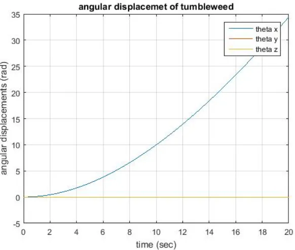
Figure 2.2 Test 1: Angular Displacement of Tumbleweed . . . 15
Figure 2.3 Test 1: Path of Tumbleweed . . . 16
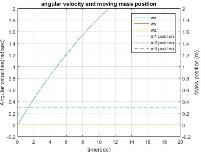
Figure 2.4 Test 1: Angular Velocity and Moving Mass Positions . . . 16
Figure 2.5 Test 2: Angular Displacement of Tumbleweed . . . 17
Figure 2.6 Test 2: Angular Velocities and Moving Mass Positions . . . 18
Figure 2.7 Test 3: Angular Displacement of Tumbleweed . . . 19
Figure 2.8 Test 3: Angular Velocities and Moving Mass Positions . . . 19
Figure 2.9 Test 4: Angular Displacement of Tumbleweed . . . 20
Figure 2.10 Test 4: Angular Velocities and Moving Mass Positions . . . 21
Figure 2.11 Test 4: Path of tumbleweed rover . . . 21
Figure 2.12 Test 5: Angular Displacement of Tumbleweed . . . 22
Figure 2.13 Test 5: Angular Velocities and Moving Mass Positions . . . 23
Figure 2.14 Test 6 : Angular Displacement of Tumbleweed . . . 24
Figure 2.15 Test 6: Angular Velocities and Moving Mass Positions . . . 24
Figure 2.16 Solidworks Model of Tumbleweed . . . 26
Figure 2.17 Solidworks Model of internal structure of Tumbleweed . . . 27
Figure 2.18 Solidworks Model of Moving Mass System . . . 28
Figure 2.19 Tumbleweed . . . 29
Figure 2.20 Tumbleweed path for moving masses out test . . . 32
Figure 2.21 Tumbleweed path for move masses out and back in test . . . 33
Figure 2.22 Path of the tumbleweed (in O frame) . . . 34
Figure 2.23 Angular Velocity of Tumbleweed . . . 35
Figure 2.24 Position of tumbleweeds at time = 0 . . . 36
Figure 2.25 Position of tumbleweeds at time = 3 . . . 37
Figure 2.26 Position of tumbleweeds at time = 7 . . . 38
Figure 2.27 Path followed by tumbleweed . . . 39
Figure 2.28 Path followed by tumbleweed because of the wind . . . 40
Figure 2.29 Angular velocities for various mass ratios . . . 42
Figure 2.30 Angular acceleration of tumbleweed for various mass ratios . . . 43
Figure 2.31 Paths taken by the tumbleweed for various wind velocities . . . 44
Figure 2.32 Angular acceleration for varying moving mass velocities . . . 45
Figure 2.33 Maximum angular velocity of the Tumbleweed . . . 46
Figure 2.34 Tumbleweed(R=2m) paths for varying wind speed and moving mass speed . . . 48
Figure 2.36 Tumbleweed(R=6m) paths for varying wind speed and moving mass
speed . . . 49
Figure 2.37 Tumbleweed(R=8m) paths for varying wind speed and moving mass speed . . . 49
Figure 2.38 Tumbleweed paths for varying wind speed . . . 51
Figure 2.39 Tumbleweed paths for varying wind speed . . . 51
Figure 2.40 Tumbleweedpaths for varying wind speed . . . 52
Figure 2.41 Tumbleweed paths for varying wind speed . . . 52
Figure 2.42 Tumbleweed paths for varying wind speed and radius . . . 53
Figure 2.43 Tumbleweed paths for varying wind speed and radius . . . 54
Figure 2.44 Tumbleweed paths for varying wind speed and radius . . . 54
Figure 2.45 Tumbleweed paths for varying wind speed and radius . . . 55
Figure 2.46 Proposed Method for Moving Masses . . . 57
Figure 3.1 Position of frames for the TRREx . . . 60
Figure 3.2 Test 1: Path followed by TRREx . . . 71
Figure 3.3 Test 1: Angular velocity of the TRREx . . . 72
Figure 3.4 Test 2: Angular displacement of the TRREx . . . 73
Figure 3.5 Test 2: Angular velocity of the TRREx . . . 74
Figure 3.6 Test 3: Angular displacement of the TRREx . . . 75
Figure 3.7 Test 3: Angular velocity of the TRREx . . . 76
Figure 3.8 Test 4: Angular displacement of the TRREx . . . 77
Figure 3.9 Test 3: Angular velocity of the TRREx . . . 78
Figure 3.10 Test 4: Path of the TRREx . . . 79
Figure 3.11 Solidworks model of lower part of TRREx arm . . . 81
Figure 3.12 Solidworks models of the upper parts of TRREx legs . . . 82
Figure 3.13 Solidworks models of wheel brackets . . . 83
Figure 3.14 Solidworks models of central support structure . . . 84
Figure 3.15 Solidworks model of one hemisphere of the TRREx . . . 86
Figure 3.16 Stress and Deformation induced in the arm . . . 88
Figure 3.17 Built up TRREx frame for one hemisphere . . . 90
Figure 3.18 Stress and Deformation induced in the arm with support . . . 91
Figure 3.19 Laid up panel . . . 92
Figure 3.20 Flow chart for laying up panels . . . 93
Figure 3.21 Wiring Diagram for the TRREx . . . 94
Figure 3.22 Fully assembled TRREx . . . 97
Figure 3.23 Rolling test for the TRREx . . . 98
Figure 3.24 TRREx in roving mode . . . 100
Figure 3.25 TRREx paths for varying arm geometries . . . 101
Figure 3.26 TRREx paths for varying arm geometries . . . 103
Figure 3.28 Slope performance of TRREx(R=1m) . . . 106
Figure 3.29 Slope performance of TRREx(R=0.3m) . . . 107
Figure 3.30 Slope performance of TRREx(R=0.6m) . . . 108
Figure 3.31 Effect of arm mass on angular velocity of TRREx(R=0.6m) . . . 110
Figure 3.32 Effect of arm mass on angular velocity of TRREx(R=0.6m) . . . 110
Figure 3.33 Effect of TRREx radius on angular velocity . . . 111
Chapter 1
Introduction
1.1
Overview of Mars Exploration
Other planets have fascinated humankind for centuries. Efforts for Mars exploration be-gan in 1960 with the Soviet Marsnik mission. Various exploration missions have since been undertaken by various space agencies around the world. NASA managed the the first successful mission with the US Viking mission in 1976. The Viking 1 lander touched down at Chryse Palanitia while Utopia Planitia was the site chosen for the for Viking 2. These Viking rovers represented the first extended mars exploration mission. The Pathfinder lander and the Sojourner rover reached Mars in July 1997. The Lander was expected to last a month while the Sojourner for just a week. However both survived for 3 months and made it to September 1997. The Pathfinders primary objective was to demonstrate the possibility of low cost landing on Mars.
water once flowed on the planet. Spirit unfortunately stopped functioning in a sand dune in March 2010. Opportunity however is expected to have a completed a twenty six mile (forty one kilometers) drive which is equivalent to a marathon. Curiosity landed on Mars in 2012 with similar objectives. India was the latest country to successfully arrive on Mars with its Mars Orbiter Mission.
A variety of vehicle architectures have been proposed in literature for rovers for mis-sions like these. However the primary architecture used is still the traditional wheeled locomotion. Most of these also use passive suspension configurations. While this config-uration is fairly effective and simple, it limits the types of terrains that the rover can successfully navigate through. There is also a significant risk of these rovers being subject to toppling over on slopes. The use of spherical rovers can help overcome these problems. Two different types of spherical architectures are considered in the cope of this study.
1.2
Tumbleweed Rover
surface of the planet. This means that the loss of a single tumbleweed, will not compro-mise the entire mission.
Over the past few years, North Carolina State University has developed and tested a number of tumbleweed earth demonstrators. The primary purpose of these was to show the capabilities of the tumbleweed architecture in an earth environment. These rover concepts displayed the ability of the tumbleweed to be pushed about by the wind and gravity but did not have any mechanism for controlling the trajectory of the rover. This study include the development and testing of an actual controllable tumbleweed earth demonstrator. By moving masses internally the center of mass of the tumbleweed rover can be shifted which in turn allows the user to control the trajectory of the rover. A mathematical model of the tumbleweed is also required to better analyse the capabilities of the tumbleweed.
1.3
Transforming Rolling Roving Explorer (TRREx)
One of the main advantages of the traditional wheeled platform is the fact that it pro-vides a stable base for data acquisition systems. To keep this advantage, the TRREx has transformation abilities which allow it to change into a normal wheeled rover. However even here it has an advantage over the conventional rovers. The presence of the arm motors allow the rover to have active suspension capabilities. This again increases the types of terrains the TRREx can traverse.
Chapter 2
Tumbleweed Rover
2.1
Developing equations of motion
It is assumed that the B frame is located at the geometric center of the tumbleweed rover. The inertial frame is represented by the O frame. Initially the axis of the B frame and O frame are parallel to each other.
There are three moving and three fixed masses present in the system. The moving masses are denoted by m1, m2 and m3, while m4, m5 and m6 are the stationary balancing masses. Location of mass1 (m1) is denoted by point P1 and can only move along the positive X axes of the B frame. Similarly m2 is located at P2 and can only move along the positive Y axes ofB frame. The third moving mass is at P3 and can only move along the positive Z axes of theB frame. The stationary masses are located midway along theB frame axis at points P4, P5 and P6.
Figure 2.1: Position of frames
{−→r P1/B}B =
R 2 0 0
{−→r P2/B}B =
{−→r P3/B}B = 0 0 R 2
{−→r P4/B}B =
−R 2 0 0
{−→r P5/B}B =
0 −R 2 0
{−→r P6/B}B =
0 0 −R 2
− →r
CM/B =
m[−→rP1/B +
− →r
P2/B +
− →r
P3/B +
− →r
P4/B +
− →r
P5/B +
− →r
P6/B]
mT
where mT is the total mass of the tumbleweed.
The O frame has to be rotated by θx about the X axis, then by θy about the Y axis, followed by θz about the Z axis. Thus the B[C]O rotation matrix obtained is as given below
[Rθx] =
1 0 0
0 cos(θx) sin(θx) 0 −sin(θx) cos(θx)
[Rθy] =
cos(θy) 0 −sin(θy)
0 1 0
sin(θy) 0 cos(θy)
[Rθz] =
cos(θz) sin(θz) 0
−sin(θz) cos(θz) 0
0 0 1
B
MatrixB[C]O is the transformation matrix used to switch between the O and B frames.
B[C]O=
c(θy)c(θz) c(θy)s(θz) −s(θy)
c(θz)s(θx)s(θy)−c(θx)s(θz) c(θx)c(θz) +s(θx)s(θy)s(θz) c(θy)s(θx) s(θx)s(θz) +c(θx)s(θy)c(θz) −s(θx)c(θz) +c(θx)s(θy)s(θz) c(θx)c(θy)
where c(θ) = cos(θ) and s(θ) = sin(θ)
O[C]B =transpose(B[C]O)
Differentiating this matrix with respect to time give the O[ ˙C]B matrix
O
[ ˙C]B = d dt(
O [C]B)
The O[ ˙C]B and B[C]O matrices are used to obtain the angular velocities
ωx=
0 0 1
B[C]O O[ ˙C]B 0 1 0 (2.2)
ωy =
1 0 0
ωz =
0 1 0
B[C]O O[ ˙C]B 1 0 0 (2.4)
The angular velocities obtained are functions of ˙θx, ˙θy and ˙θz.Equations (2.2), (2.3) and (2.4) are solved to obtain the expressions for ˙θx, ˙θy and ˙θz. That gives the equations for the the first three states.
The inertia tensor for the body of the tumbleweed (without the masses) is obtained from Solidworks and is as follows:
˜
If = 1.21
− →
i B−→i B+ 1.21−→j B→−j B+ 1.21−→kB−→kB
As all the position vectors are know with respect to theB frame, the transport theorem is used to calculate the velocities in theO frame. The velocities are still being expressed in terms of the B frame.
O−→v B/O =
B d dt(
− →r
B/O) + (
O−→ωB× −→r B/O)
O−→v
P1/B =
Bd dt(
− →r
P1/B) + (
O−→v
P2/B =
Bd dt(
− →r
P2/B) + (
O−→ωB× −→r P2/B)
O−→v
P3/B =
Bd dt(
− →r
P3/B) + (
O−→ωB× −→r P3/B)
O−→
v P4/B =
Bd dt(
− →r
P4/B) + (
O−→
ωB× −→rP4/B)
O−→v
P5/B =
Bd dt(
− →r
P5/B) + (
O−→ωB× −→r P5/B)
O−→v
P6/B =
Bd dt(
− →r
P6/B) + (
O−→ωB× −→r P6/B)
Angular momentum of the tumbleweed body is obtained by using the inertia tensor
O−→h
body,B = ˜If.OωB
same direction. So their product is zero and hence they do not contribute towards the angular momentum of the tumbleweed frame.
Similarly the angular momentum of every moving mass can also be calculated. All of the angular momenta are being expressed in the B frame.
O−→
hP1,B =−→rP1/B ×(m(
O−→ vB/O +
O−→ vP1/B))
O−→h
P2,B =−→rP2/B ×(m(
O−→v B/O +
O−→v P2/B))
O−→h
P3,B =−→rP3/B ×(m(
O−→v B/O +
O−→v P3/B))
O−→
hP4,B =−→rP4/B ×(m(
O−→ vB/O +
O−→ vP4/B))
O−→h
P5,B =−→rP5/B ×(m(
O−→v B/O +
O−→v P5/B))
O−→h
P6,B =−→rP6/B ×(m(
O−→v B/O +
Summing all of these gives us the total angular momentum of the tumbleweed.
O−→h B =O
− →
hf rame,B+O
− →
hP1,B+O
− →
hP2,B+O
− →
hP3,B+O
− →
hP4,B+O
− →
hP5,B+O
− →
hP6,B (2.5)
The external torque is obtained by differentiating this angular momentum term in theO frame. − →τ ext= Bd dt( O−→h
B) + (O−→ωB×O
− →
hB) (2.6)
The external torques acting on the system are due to gravity and wind force. Wind force acts along the direction of the wind and its magnitude is as follows
Wind force
Fw = 0.5(ρ)(Area)(Cd)(−→v rel.−→vrel)
where
ρ = density of air
− →v
rel = relative velocity of wind with respect to point B on tumbleweed
− →τ
ext = (
− →
R ×−→Fw) + (−→rCM/B ×
− →
Fgrav) (2.7)
where
− →
Fgrav = force of gravity
− →
R = Position vector for center of tumbleweed(point B)
Compare the right hand sides of equation (2.6) and (2.7). The obtained set of equa-tions are solved to get equaequa-tions for the ˙ωx, ˙ωy and ˙ωz. These are the remaining three state equations needed to simulate the motion of the system. A no slip condition has been imposed on the tumbleweed. So the linear position of the tumbleweed is equal to the product of the radius and the angular position of the tumbleweed.
2.2
Simulation results for test cases
The equations obtained for the angular accelerations and angular velocities are numer-ically integrated to predict the motion of the tumbleweed rover subjected to various conditions. MATLAB’s ode solver is used to numerically integrate the equations. A few test cases are presented below to verify the correctness of the model. For all of the test cases, the B frame and the O frame are lined up with each other at the start.
2.2.1
Constant wind loading
From 2.2 and 2.4 it is seen that the tumbleweed rover keeps on rolling along theyo axis.
Figure 2.2: Test 1: Angular Displacement of Tumbleweed
Figure 2.3: Test 1: Path of Tumbleweed
2.2.2
Breaking by Moving a Mass
The tumbleweed is initially given a counterclockwise angular velocity of 0.3 rad/sec about the yo axis. After 5 seconds mass M1 is moved outward along the positive xb axis and then pulled back in.
From figure 2.6 it is seen that the mass starts to move the angular velocity starts
Figure 2.5: Test 2: Angular Displacement of Tumbleweed
Figure 2.6: Test 2: Angular Velocities and Moving Mass Positions
2.2.3
Move one mass upwards
The tumbleweed is completely stationary. After 3 seconds the mass M3 is moved out along the positive zB axis and then brought back in.
Figure 2.7: Test 3: Angular Displacement of Tumbleweed
2.2.4
Move the tumbleweed along an axis
The tumbleweed is initially stationary. After 3 seconds mass M1 is moved out along the xB axis and then brought back in. At time = 8 seconds, mass M3 is moved out and brought back in along thezB axis.
As the mass M1 moves, it creates a torque about the yO axis which causes the
tum-Figure 2.9: Test 4: Angular Displacement of Tumbleweed
Figure 2.10: Test 4: Angular Velocities and Moving Mass Positions
2.2.5
Oscillatory behavior about Y axis
At time =0, the mass M1 is positioned at 0.5 meters along the positive xB axis and kept there throughout the the simulation.
Figure 2.13: Test 5: Angular Velocities and Moving Mass Positions
As seen from figure 2.13 the angular velocity of the tumbleweed keeps increasing and decreasing with time. This indicates that tumbleweed rolls back forth. Finally the angular velocity damps out to zero and the tumbleweed will settle down with the mass M1 pointing downwards.
2.2.6
Oscillatory behavior about x axis
Figure 2.14: Test 6 : Angular Displacement of Tumbleweed
As seen from figure 2.15 the angular velocity of the tumbleweed keeps increasing and decreasing with time. This indicates that tumbleweed rolls back forth. Finally the angu-lar velocity damps out to zero and the tumbleweed will settle down with the mass M2 pointing downwards. The damping out of the tumbleweed is due the effect of friction. Rolling frcition between the tumbleweed and the ground, causes loss of energy which causes the tumbleweed motion die down.
2.3
Design and Construction of Proof of Concept
Tumbleweed Rover
Figure 2.16: Solidworks Model of Tumbleweed
Figure 2.17: Solidworks Model of internal structure of Tumbleweed
Solidworks model of this is as shown in figure (2.17).
Figure 2.18: Solidworks Model of Moving Mass System
The sails are attached to the central and the peripheral pipes by means of zip ties. In future, this should be replaced by Velcro as it will allow the sails to be detached and reattached without having to cut off the zip ties. The sails are made up of nylon cloth and are cut in the shape of quadrants of a circle.
Figure (2.19) shows the the assembled proof of concept tumbleweed. To spherical shape of the tumbleweed is obtained by bending the PVC pipes to form circular arcs. These small arcs are attached to each other by the use of pre-made 4 way connection crosses. At the top and bottom of the sphere there are a total of 8 pipes. Four of these are fixed to each other by using a 4 way cross segment and the remaining four are fixed to this by using PVC cement. If the tumbleweed is made to be a solid sphere then sails cannot be used. The drag coefficient of a flat circular surface ( 1.75 - 2.0) is much higher than the drag coefficient of a spherical surface ( 0.5). Thus the amount of force generated by the wind on the tumbleweed is less in case it is a solid spherical shell. Hence a caged structure is used. However the use of cage structure does present the possibility of the tumbleweed getting stuck on a rock. Aluminum brackets are used to attach the central structure to the outer spherical cage. The bolts used as idler shafts also double up as the bolts used to attach the brackets.
The motors used to move the masses are controlled by an Arduino Nano. This Arduino is connected to an XBEE mounted on board the tumbleweed. This allows the user to send signals to the motors remotely by using a computer. The central pipes which do not contain the moving masses, act as the storage place for the Arduino, Xbee and the battery.
the mass is being fixed to the belt.
2.4
Testing of Tumbleweed Rover
Various tests were carried out using the constructed tumbleweed rover to see its response to the masses moving. These includes the tumbleweed starting from a static position, as well as one with the tumbleweed rolling.
2.4.1
Masses moving outward along the two pipes
Figure 2.20: Tumbleweed path for moving masses out test
2.4.2
Masses moved out and then back in
The tumbleweed is initially stationary. The masses are able to move along thexB and yB axis. The tumbleweed is positioned such that the xB -yB plane is parallel to the ground. Both masses are then moved outward and then moved back in.
Figure 2.21: Tumbleweed path for move masses out and back in test
energy during the impact and does not have enough angular velocity left to keep rolling forward. The tumbleweed falls slightly to one side as there is a slight imbalance on ac-count it not being an exact sphere. During the test it also observed that the tumbleweed moves along a line about 45 degrees to the positive xO axis in the first quadrant.
The same conditions are plugged into the MATLAB model for the tumbleweed developed before.
Figure 2.23: Angular Velocity of Tumbleweed
From figure (2.22) we see that as per the simulation, the tumbleweed follows a path which bisects the angle between the positive xO and positive yO axis. This direction is same as the path actually observed. The values of displacement are different as the actual tumbleweed loses a lot of energy when it hits the central ring. This loss of energy is not accounted for in the MATLAB model.
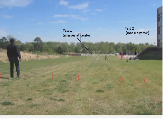
2.4.3
Rolling down a slope test
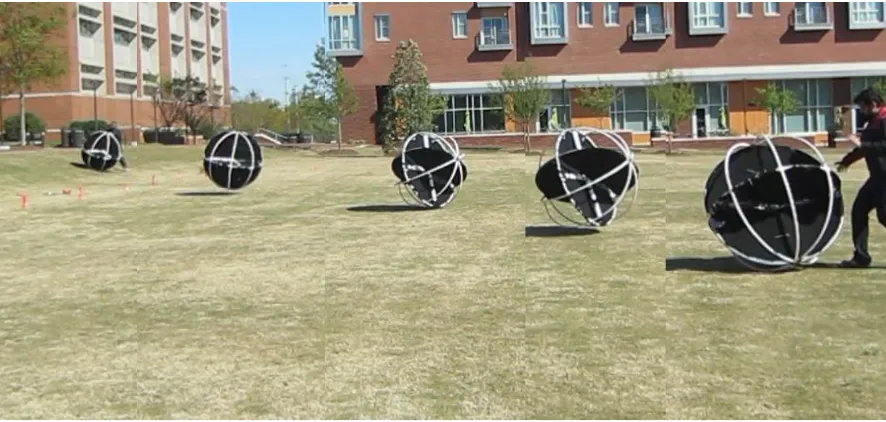
constant wind force on the tumbleweed. For part one of the test the masses were fixed at the center and then the tumbleweed was let go. The path that it followed down the slope was recorded by the use of two cameras. The tumbleweed was brought back up again and then let go. However this time, the masses were moved outward along the xB and theyBaxis. The path of the tumbleweed was again recorded by the same two cameras.
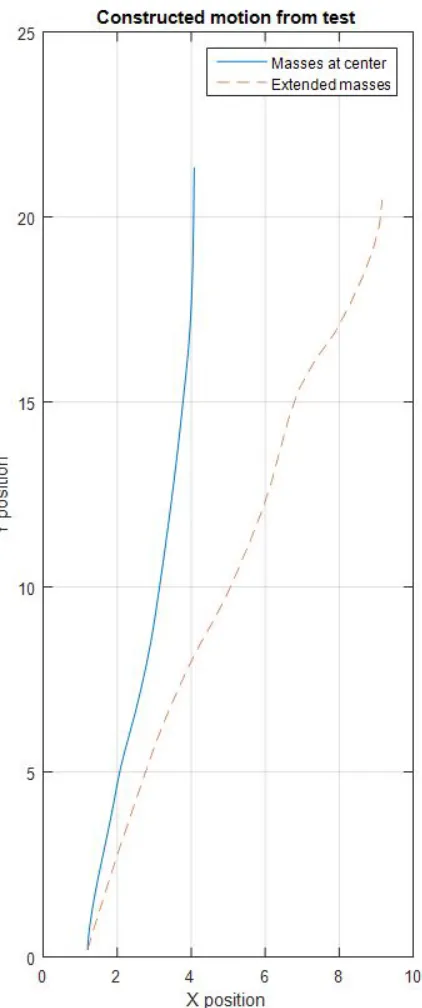
It is seen that the tumbleweed goes in roughly a straight line when the masses are fixed in the center. However, the tumbleweed keeps on curving towards the right in part two. This deviation in path can be seen in the figures below. These are photos taken from the test, which have been overlain over each other to facilitate comparison between the the position of the tumbleweeds during the the two parts of the test.
Figure 2.26: Position of tumbleweeds at time = 7
From (2.24), (2.25) and (2.26) it can be seen that the two start at the same location and then diverge as the one with the moving masses curves towards the right. When the masses are in the center, the tumbleweed should go in a line straight ahead. But actually it deviates to the right a bit. This is because the slope that was used to test, also has a slight inclination that way. The important point to note is that the path of the tumbleweed with the extended masses is always to the right of the tumbleweed with all the masses at the center.
2.4.4
Wind test
The aim of this test is to demonstrate the ability of the tumbleweed to be pushed around by the wind because of the wind. Sails are cut out from nylon cloth and attached to the tumbleweed. Ideally the sails would be along the xB-yB, yB-zB and xB-zB planes. However for this test, sails were attached only along the yB-zB and xB-zB planes. The tumbleweed was then placed on the ground in front of the OVAL and then let go.
Figure 2.28: Path followed by tumbleweed because of the wind
25 meters in 6 seconds. It is also able to travel up inclines under the action of wind. This motion of the tumbleweed under the action of wind is shown in figure (2.28). It is also seen from this test that the tumbleweed has a tendency to bounce as it gains velocity. This might be the result of it not having a smooth spherical surface.
2.5
Effect of moving mass value on Tumbleweed
Re-sponse
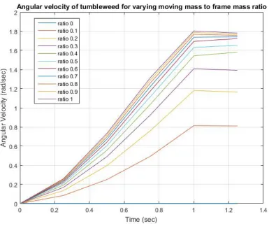
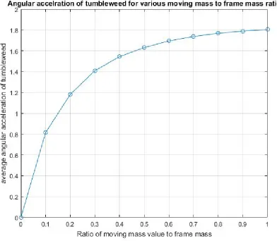
Selecting the mass value for moving masses is integral to the development of the tumble-weed. To enable the selection of proper mass value, the response of the tumbleweed for various mass values was evaluated. The ratio of the moving mass value to the frame mass was varied from 0 to 1. In all the cases the distance through which the mass is moved, and the speed with which the mass is moved is kept constant. The angular velocity and the average angular acceleration due to this movement is plotted.
From figure (2.30) it can be seen that as ration goes on increasing, the angular accel-eration also increases. This increased angular accelaccel-eration implies a faster response time for the tumbleweed. However it is also evident from the graph, that the rate of increase in acceleration goes on decreasing. The acceleration values tend to plateau off once the ratio is more than 0.7. Based of just this graph it seems that increasing the value of the moving mass while keeping the value of the chassis mass constant is highly desirable.
Figure 2.29: Angular velocities for various mass ratios
Figure 2.30: Angular acceleration of tumbleweed for various mass ratios
2.6
Effect of wind velocity on turn radius
To study this effect, the wind velocity is varied while all the other parameters like
Figure 2.31: Paths taken by the tumbleweed for various wind velocities
2.7
Effect of moving mass velocity on Tumbleweed
performance
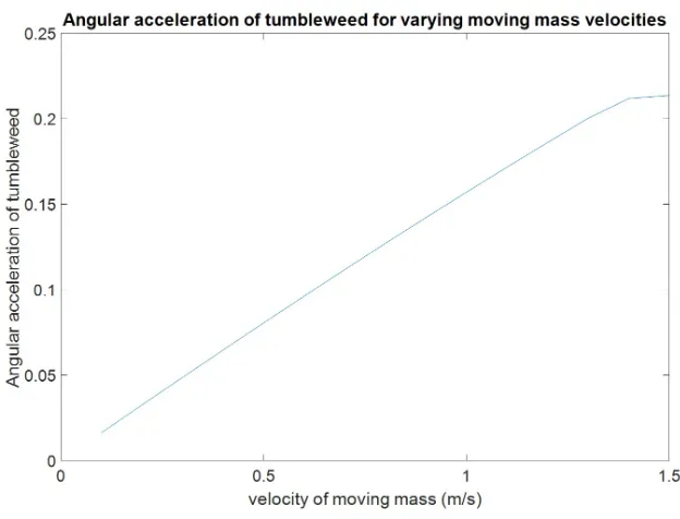
The moving masses are the main control elements for the tumbleweed. The rate at which these masses move, will have a direct bearing on the handling of the tumbleweed. The faster you move these masses, the faster the torque value acting on the tumbleweed changes. To observe the effect of these masses, the moving mass velocity was varied from 0.1 m/s to 1 m/s. The moving masses are moved out and then back inside after they reach the end. The angular acceleration and the angular velocity of the tumbleweed are the parameters of interest in this test.
The initial acceleration of the tumbleweed increases as the velocity of the moving mass
Figure 2.32: Angular acceleration for varying moving mass velocities
Figure 2.33: Maximum angular velocity of the Tumbleweed
show a different trend. As figure (2.32) shows, the tumbleweed in which the masses move slower reaches a higher angular velocity. A possible explanation for this is that as the masses move slower, they are in their extended positions for longer. This implies that the tumbleweed is accelerating for longer which may result in a higher top angular ve-locity. However as expected, moving the masses faster gets a quicker response from the tumbleweed, which will make it more maneuverable. However moving the masses faster will increase the current draw on the batteries, thus reducing their life.
2.8
Parametric Studies using tumbleweed model
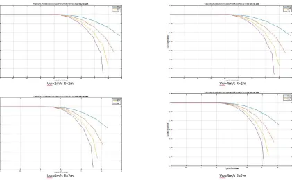
tum-bleweed will also get heavier as more material will be needed to build the rover. To try and characterize the effect of these parameter, a parametric study is carried out using the mathematical model of the tumbleweed. For any given part of the study, two parameters will be kept fixed and the third quantity will be varied. Four values of each parameter will be tried giving a total of 64 combinations from which inferences can be drawn.
2.8.1
Varying moving mass speed
Figure 2.34: Tumbleweed(R=2m) paths for varying wind speed and moving mass speed
Figure 2.36: Tumbleweed(R=6m) paths for varying wind speed and moving mass speed
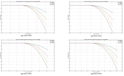
2.8.2
Varying the wind speed
Figure 2.38: Tumbleweed paths for varying wind speed
Figure 2.40: Tumbleweedpaths for varying wind speed
2.8.3
Varying radius of tumbleweed
Changing the radius of the tumbleweed changes the distance the moving masses have to travel. Also it changes the moment caused by the masses on the tumbleweed. The force due to the wind is aslo directly dependent on the square of the radius. thus the radius value affects the rolling properties of the tumbleweed a great deal.Figures (2.43), (2.44) and (2.45) show the effect of variying the tumbleweed radius on the path taken by the tumbleweed. Due to an increase in cross sectional area, the wind force becomes more dominant as the radius of the tumbleweed goes on increasing.
Figure 2.43: Tumbleweed paths for varying wind speed and radius
2.9
Conclusions and Lessons Learned
2.9.1
Support for moving masses
The entire weight of the moving masses is currently borne by just the belts. This causes the moving masses to move about a lot in various direction. If a supporting guide rail is added, it will take the load of the mass and constrain it to move along only one direction. It would be beneficial if the masses are supported by the guide and the belts are only responsible for pulling it along one axis.
2.9.2
Include a Tensioner
Figure 2.46: Proposed Method for Moving Masses
Figure 2.46 shows a proposed design which includes both the points stated above. The rod will bear the weight of the mass while the springs will ensure that the belt remains under tension. In addition to providing support, the support rod can also be used to sense position of the mass along the axis.
2.9.3
Cage structure
of the created cage structure. Additional small rings should also be added at varying heights to increase the rigidity of the tumbleweed. Also there needs to be some research done to come up with a better alternative material for PVC. The PVC pipes bend and flex a lot under load, which greatly affects the rolling characteristics of the tumbleweed.
2.9.4
Need for controller and feedback on mass position
Chapter 3
Transforming Rolling Rover
Exploration Rover (TRREx)
3.1
Deriving equations of Motion
The B frame is located at the geometric center of the sphere. The inertial frame is rep-resented by the O frame. Initially the axis of the B frame and O frame are parallel to each other.
Figure 3.1: Position of frames for the TRREx
any arm from its hinge point is same. This distance is denoted by lc. Angles made by a leg frame with respect to B frame are denoted by θ and follow the same numbering convention. So θ11 is the angle by which F11 will have to be rotated to align with the B frame.
Based on this the position vectors can be defined as follows:
− →r
C11/B = (R−lccos(θ11))
− →
j B+ (lcsin(θ11))
− →
kB
− →r
C12/B = (R−lccos(θ12))
− →
j B−(lcsin(θ12))
− →
− →r
C21/B = (R−lccos(θ21))
− →
i B+ (lcsin(θ21))
− →
kB
− →r
C22/B = (R−lccos(θ22))
− →
i B−(lcsin(θ22))
− →
kB
− →r
C31/B = (−R+lccos(θ31))
− →
j B+ (lcsin(θ31))
− →
kB
− →r
C32/B = (−R+lccos(θ32))
− →
j B−(lcsin(θ32))
− →
kB
− →r
C41/B = (−R+lccos(θ41))
− →
i B+ (lcsin(θ41))
− →
kB
− →r
C42/B = (−R+lccos(θ42))
− →
i B−(lcsin(θ42))
− →
kB
From these vectors, the position vector for the center of mass of the TRREx from point B can be calculated.
− →r
CM/B =
m(−→rC11/B +
− →r
C12/B +
− →r
C21/B +
− →r
C22/B +
− →r
C31/B +
− →r
C32/B +
− →r
C41/B +
− →r
C42/B)
mT
where mT is the total mass of the tumbleweed.
[Rθx] =
1 0 0
0 cos(θx) sin(θx) 0 −sin(θx) cos(θx)
[Rθy] =
cos(θy) 0 −sin(θy)
0 1 0
sin(θy) 0 cos(θy)
[Rθz] =
cos(θz) sin(θz) 0
−sin(θz) cos(θz) 0
0 0 1
B[C]O = [Rθ
x][Rθy][Rθz] (3.1)
∴ B[C]O =
c(θy)c(θz) c(θy)s(θz) −s(θy)
c(θz)s(θx)s(θy)−c(θx)s(θz) c(θx)c(θz) +s(θx)s(θy)s(θz) c(θy)s(θx) s(θx)s(θz) +c(θx)s(θy)c(θz) −s(θx)c(θz) +c(θx)s(θy)s(θz) c(θx)c(θy)
where c(θ) = cos(θ) and s(θ) = sin(θ)
O[ ˙C]B = d dt(
O[C]B)
The O[ ˙C]B and B[C]O matrices are used to obtain the angular velocities
ωx=
0 0 1
B[C]O O[ ˙C]B 0 1 0 (3.2)
ωy =
1 0 0
B[C]O O[ ˙C]B 0 0 1 (3.3) ωz =
0 1 0
B[C]O O[ ˙C]B 1 0 0 (3.4)
Equations (3.2), (3.3) and (3.4) are solved to obtain the expressions for ˙θx, ˙θy and ˙θz. That gives the equations for the the first three states. The inertia tensor for the body of the TRREX(without the arms) can be expressed as follows
[ ˜If]B =
If x 0 0 0 If y 0 0 0 If z
The inertia tensor for every arm (around its own center of mass) can be found in the arm frame wit the help of SOLIDWORKS.
Inertia tensor for arm11 inF11 frame is
[ ˜Ic11]F11 =
Ix11 0 0
0 Iy11 0
0 0 Iz11
The rotation matrix to get from F11 to B is as follows
B[C]F11 =
1 0 0
0 cos(−θ11) sin(−θ11) 0 −sin(−θ11 cos(−θ11)
By pre and post multiplying the inertia tensor with the rotation matrix, the inertia tensor of the arm as expressed in the B frame is obtained
[ ˜Ic11]B =
B[C]F11[ ˜I
c11]F11
F11[C]B (3.5)
By using the same procedure, inertia tensors for all the other arms can be found and expressed with respect to the B frame. Four of the tensors have to be rotated about the yB axis while the remaining four are rotated about the xB axis.
[ ˜Ic12]B = B
[C]F12[ ˜I
c12]F12
[ ˜Ic21]B =
B [C]F21[ ˜I
c21]F21
F21[C]B
[ ˜Ic22]B =
B [C]F22[ ˜I
c22]F22
F22[C]B
[ ˜Ic31]B =B [C]F31[ ˜Ic31]
F31
F31[C]B
[ ˜Ic32]B =
B [C]F32[ ˜I
c32]F32
F32[C]B
[ ˜Ic41]B =
B [C]F41[ ˜I
c41]F41
F41[C]B
[ ˜Ic42]B =B [C]F42[ ˜Ic42]
F42
F42[C]B
O−→v B/O =
Bd dt(
− →r
B/O) + (
O−→ωB× −→r B/O)
O−→v
C11/B =
Bd dt(
− →r
C11/B) + (
O−→ωB× −→r C11/B)
O−→
vC12/B =
Bd dt(
− →r
C12/B) + (
O−→
ωB× −→rC12/B)
O−→v
C21/B =
Bd dt(
− →r
C21/B) + (
O−→ωB× −→r C21/B)
O−→v
C22/B =
Bd dt(
− →r
C22/B) + (
O−→ωB× −→r C22/B)
O−→
vC31/B =
Bd dt(
− →r
C31/B) + (
O−→
ωB× −→rC31/B)
O−→v
C32/B =
Bd dt(
− →r
C32/B) + (
O−→v
C41/B =
Bd dt(
− →r
C41/B) + (
O−→ωB× −→r C41/B)
O−→v
C42/B =
Bd dt(
− →r
C42/B) + (
O−→ωB× −→r C42/B)
Angular momentum of the TRREx frame is obtained by using the inertia tensor for the frame
O−→h
f rame,B = ˜If.O−→ωB
The angular momentum for each of the arms is also obtained as follows
O−→
h11,B =−→rc11/B×(m(O−→vB/O +
O−→
vC11/B)) + ˜Ic11.
O−→ ωB
O−→h
12,B =−→rc12/B×(m(O−→vB/O +
O−→v
C12/B)) + ˜Ic12.
O−→ωB
O−→
h21,B =−→rc21/B×(m(O−→vB/O +
O−→
vC21/B)) + ˜Ic21.
O−→h
22,B =−→rc22/B×(m(O−→vB/O +
O−→v
C22/B)) + ˜Ic22.
O−→ωB
O−→h
31,B =−→rc31/B×(m(O−→vB/O +
O−→v
C31/B)) + ˜Ic31.
O−→ωB
O−→
h32,B =−→rc32/B×(m(O−→vB/O +
O−→
vC32/B)) + ˜Ic32.
O−→ ωB
O−→h
41,B =−→rc41/B×(m(O−→vB/O +
O−→v
C41/B)) + ˜Ic41.
O−→ωB
O−→h
42,B =−→rc42/B×(m(O−→vB/O +
O−→v
C42/B)) + ˜Ic42.
O−→ωB
The total angular momentum of the TRREx is found by adding all the above angular momentum terms
O−→h B =O
− →
hf rame,B+O
− →
h11,B+O
− →
h12,B+O
− →
h21,B+O
− →
h11,B+O
− →
h31,B+O
− →
h32,B+O
− →
h41,B+O
− →
h42,B (3.6)
− →τ
ext= Bd
dt( O−→h
B) + (O−→ωB×O
− →
hB) (3.7)
The external torque acting on the TRREX is due to gravity. Force due to gravity is easily expressed in theO frame. This force will have to be rotated into the B frame.
Thus the external torque acting on the TRREx is
− →τ
ext =rCM/B × {Fgrav} (3.8)
Compare the right hand sides of equation (3.7) and (3.8). The obtained set of equations are solved to get equations for the ˙ωx, ˙ωy and ˙ωz. These are the remaining three state equations needed to simulate the motion of the system.
3.2
Simulation Results for the TRREx
˙ θx ˙ θy ˙ θz ˙ ωx ˙ ωy ˙ ωz
= [B]×
θx θy θz ωx ωy ωz
The B matrix contains all the coefficients for the variables and is constructed by collect-ing the coefficients of the terms from the equations of motion.
An inbuilt ode solver from MATLAB (ode23) is used to numerically integrate these equations to obtain angular position and angular velocity at every time step. The motion of the arm has to be prescribed by the user and is an input to the code. The position and the velocity of the arms at every time step has to be defined by the user before the simulation code can be run. To verify the correctness of the model developed, a few test cases were run using it. The test cases represent input conditions to which the expected response of the TRREx is known. So in other words, these conditions provide a sanity check for the mathematical model. The results obtained from running these tests are presented in the following subsection.
3.2.1
Opening one arm
When the TRREx opens one of its arms, the center of mass will shift towards the
Figure 3.2: Test 1: Path followed by TRREx
Figure 3.3: Test 1: Angular velocity of the TRREx
3.2.2
Opening opposite arms
The TRREx is kept stationary. It is aligned so that the B frame and the O frame are lined up with each other perfectly. Then two arms which are located opposite to each other are opened at the same. Both the arms are located in the same plane and in the upper hemisphere of the TRREx.
Figure 3.4: Test 2: Angular displacement of the TRREx
Figure 3.5: Test 2: Angular velocity of the TRREx
3.2.3
Using arms to brake
One of the functions the moving arms have to perform is to provide braking action to stop the TRREx from rolling. This test demonstrates the ability of the TRREx to stop rolling and start moving the other way by opening its arms.
Figure 3.6: Test 3: Angular displacement of the TRREx
Figure 3.7: Test 3: Angular velocity of the TRREx
3.2.4
Change direction using arms
The TRREx should be able to change the direction in which it is rolling by opening its arms. To obtain this, arms have to be opened in a plane perpendicular to the plane in which it is rolling.
Figure 3.8: Test 4: Angular displacement of the TRREx
Figure 3.9: Test 3: Angular velocity of the TRREx
3.2.5
Turning characteristics in varying gravity fields
Figure 3.10: Test 4: Path of the TRREx
3.3
Design and Development of Proof of Concept
TRREx
control and is expected to be controlled manually through wireless communication.
The development of the entire TRREx can be divided into three main section, the frame, panels and the electronics.
3.3.1
Frame and sub structure
The frame and the substructure includes all the components made up off aluminum. This includes the moving arms and all the other central structural elements used to mount other components on.
Arms
The arms are the moving components of the TRREx and are used to change the posi-tion of the center of mass. A total of eight arms are required out of which six will have wheels on them. Arms with wheels are referred to as live arms, and the other two are dead arms. The wheels are not necessary for rolling mode, but are required for the roving mode.
Figure 3.11: Solidworks model of lower part of TRREx arm
Wheel Brackets
Figure 3.13: Solidworks models of wheel brackets
the arms open in a plane perpendicular to the other four. These two configurations are shown in figure (3.13).
Central support structure
Figure 3.14: Solidworks models of central support structure
down the arm brackets. Radial holes are also drilled into the ring. These holes enable the rectangular pieces to be attached to the ring. The central part of the TRREx has to provide a platform so that various instruments like drivers, batteries etc can be securely mounted. The rectangular pieces of aluminum are arranged in the shape of a cross for this purpose. Each hemisphere gets one cross. While the TRREx is being assembled it should be ensured that the two crosses line up with each other perfectly. The cross is made up off one long piece of aluminum and two shorter rectangular pieces. One end of the shorter pieces is bolted to the ring. Both ends of the long piece are bolted to the ring. Holes are drilled into the sides of these rectangular pieces. Brackets for the motor drivers and the Arduino NANO are fixed using these holes. However the motors cannot be mounted to these pieces directly. The design constraint dominating this decision is the amount of angular movement allowed by the hinges attached to the bottom end of the motor. To provide the correct angle to mount the motors, triangular wedges are used. Two types of wedges are used. One of them looks like an extruded triangle while the other looks like and extruded trapezium. The trapezoidal shaped wedge serves a dual purpose. Not only does it provide a surface to mount the motors, but also fixes the two free ends of the shorter rectangular pieces to each other. The sloping surfaces of the wedges have four holes made on them, which are used to bolt the motors to them. The smaller wedges are fixed to the longer rectangular piece with bolts. The same arrangement is repeated for the other hemisphere.
An identical second hemisphere will go under this one to complete the structure of the TRREx. In the current model of the TRREx, there is no provision for the two halves to be able to separate automatically. So for this version, the two halves will be bolted to each other while it is in the rolling mode. These bolts will have to be removed manually by the user to disconnect the two halves and then put it in the roving mode.
Figure 3.15: Solidworks model of one hemisphere of the TRREx
3.3.2
Panels
The outer spherical surface of the rover is made up of fibreglass panels. The entire spher-ical surface will be divided into octants. Each individual panel will be the size and shape of one - eight sphere. The panels are responsible for providing a smooth surface for the TRREx to roll on. In absence of the panels, the TRREx is subject to getting stuck on obstacles like rocks. The panels protect the interior of the TRREx from outside obstacles.
Figure 3.19: Laid up panel
cut off during sanding the panels. The panels are attached to the arm with the help of bolt. To allow for this two holes are drilled into each panel.
Figure 3.20: Flow chart for laying up panels
3.3.3
Actuation and control
am-peres. A factor working in favor of selecting these motors is the fact that the linear piston can be detached and connected to other motors with different specifications. This may al-low reduction in overall mass or modification in TRREx performance by changing motors.
These motors are controlled by the Sabertooth 2X25 motor driver made by Dimension
Figure 3.21: Wiring Diagram for the TRREx
positions. Initially PWM control signal was attempted to specify the velocity at which the motrs should operate. The main drawback of using this technique is the fact that it requires two analog pins of the Arduino per driver. This will mean that a single Arduino NANO will not be sufficient to provide control input to all the drivers. If serial signals are used, only one digital pin per driver is needed. This implies that a single Arduino is now sufficient. So the drivers will be set into serial configuration and serial control inputs are used. The S1 pin of each driver is connected to a digital pin on the micro-controller. Four power sources, one for each motor driver, is present inside the TRREx. The Arduino is powered through the 5V pin on the driver. The basic motor driver control program was written in C using the Arduino IDE. The user needs to have the ability to control the TRREx actuators manually. XBEEs are used to allow for wireless transmission between the user and the Arduino. The user will be controlling the TRREx witha remote con-troller which has a XBEE connected to it. The other XBEE is connected to the Arduino and is present on the TRREx. The wiring diagram for the electronics is shown in figure (3.21). The Arduino code used to control the motors is included in appendix at the end. The Arduino code is written to control the speed of the motor and not the position. By setting the voltages being transmitted to the motor , the speed with which the motors move and thier direction can be controlled. This presents a problem. The motor velocity can be easily set to zero by setting input voltage to zero. However when the voltage is set to zero, the motor will not provide any holding torque which allows the arms to dragged out by external forces.
Each hemisphere has four motors which are controlled by two motor drivers. The motor drivers are present in diagonally opposite quadrants. Brackets are made out out plastic angles to mount the motor drivers. These get bolted onto the central cross. The Arduino is also mounted onto one of the crosses in a similar manner. After all the drivers are in place, the arms and motors get mounted and connected to each other. The wheels are attached on to the wheel brackets to complete the skeletal setup of the rover. The batteries are stuck onto the linear moors with the help of duct tape. This is not an ideal solution and a better mounting place needs to be developed. The panels then get bolted onto the arms to close up and complete the assembly of a hemisphere. The two hemispheres then get fixed to each other using bolts. In the final version of the TRREx, the two hemispheres will be connected to each other with a hinge mechanism which will allow the rover to open up. The fully assembled TRREx is shown in figure (3.22). The TRREx shown in this figure is currently in the rolling mode.
3.4
Testing of Proof of Concept TRREx
The validity of the results shown in the simulations needs to be backed up by experiments. To demonstrate the various capabilities of the built TRREx some basic tests are carried out using the constructed rover.
3.4.1
Test for rolling ability of the TRREx
Figure 3.22: Fully assembled TRREx
electronics and then the panels are fixed to close the TRREx up. The corresponding other Xbee is connected to the computer and XCTU program is used to open up a connection between the two Xbees. The camera is setup and the command to open up two adjacent panels is sent to the rover.
Figure 3.23: Rolling test for the TRREx
that the panels flex and bend a lot. This means that the rolling surface is not completely spherical which adversely affects the rolling characteristics. Slight bending is observed in the TRREx arms even with the reinforcement in place. Another issue observed during the testing was the current draw acting on the batteries. The batteries connected to the actuated arms have a life of about 15 minutes which is less than desirable.
3.4.2
Demonstrating Roving mode
Figure 3.24: TRREx in roving mode
3.5
Parametric studies using the TRREx model
The main parameters which affect the movement of the TRREx are the radius of the TRREx, the properties of the arms and the weight of the rover. These studies were carried out to see how the TRREx performs for various combinations of these parameters. These effects can be seen in the following plots.
So shifting the center of mass further from the hinge point in desirable.
Figure 3.25: TRREx paths for varying arm geometries
3.5.3
Effect of radius and arm speed on hill climb ability
3.5.4
Changing arm mass
Figure 3.31: Effect of arm mass on angular velocity of TRREx(R=0.6m)
3.5.5
Effect of changing radius
Radius is the primary geometric feature of the TRREx. The effect of changing radius on the response of the TRREx is examined in this section. The radius of the rover and mass of the rover are directly linked. As the radius increases, the mass also increases. Initially the TRREx is at rest. Then an arm is opened. htis causes the TRREx to start rolling in that direction. Figure (3.33) shows the angular velocity of the rover. From this it can be seen that the larger TRREx accelerates slower. The additional mass caused by increasing the size causes the larger rover to be slower.
3.6
Conclusion and lessons learned
The testing of the first fully spherical TRREx rover revealed some major flaws in the design of the the rover. Several important lessons were learned during this process and they are outlined in the sub-sections listed below.
3.6.1
Change in design process
3.6.2
Change the arm design
The TRREx arms have to support the weight the rover as it rolls over the arms. The arm segment above the motor bracket form a cantilever beam. The primary structural load acting on the arms will be a bending moment in the arm due to the weight of the rover. This moment will be maximum when the weight is at the free end of the arm. The tensile stress approximation equation is as follows:
σ =M ×c/I (3.9)
Using this equation and the safe stress value for aluminum 6061, each arm can safely support a force of 47 pounds. The estimated weight of the TRREx after the actual motors came in is about 160 pounds. This clearly shows that the current arm design is inade-quate and needs to be modified. This is happening as the maximum moment of inertia is in a plane perpendicular to the plane in which the load is acting.
3.6.3
Adding rigidity to the panels
The rolling test for the TRREx showed that the panels were bending and flexing a lot. Currently the panels are held onto the arm by bolts along the center line of the panel. This leaves a lot of cantilever structure on both sides. This causes the a lot of bending moment on the overhanging part of the panels. Once the panels start flexing, the rover is no longer a sphere and so it does not roll properly.
To prevent this, the outer edges of the fiberglass panels need to be supported. This can
Figure 3.34: Fixed supports for panels
and so it is not desirable to place them under additional stress. The second idea is to add additional fixed half arms to the rings. Half arms with the same radius of curvature as the arms will bolted onto the ring in between the existing arms. These will be located such that the edges of the panels can rest on them when the arms are closed. These half arms are stationary arms and cannot be moved. The panels will not be fixed onto hem. They will only rest against these projections when they are under load. These projections will prevent the panels from being pushed into the sphere and thus will help to maintain the spherical shape. These half arms will also help to reduce the load acting on the arms and the panels, thus increasing the safety factor for all these components. These supports are shown in figure (3.34). The holes are made into the panel supports to try and save weight and are not strictly required.
3.6.4
Shift center of mass of arms
3.6.5
Keeping radius constant
REFERENCES
[1] J. J. Duistermaat. (2004) Chaplygin’s sphere. ArXiv Mathematics e-prints
[2] Meirovitch. (1970) Methods of Analytical Dynamics. Dover.
[3] J. Leigh. (2007) Design and Modeling of Mars Tumbleweed Rover. Thesis, NC State University
[4] Lionel Ernest Edwin. (2007) Transforming Roving-Rolling Explorer (TRREx) for Planetary Exploration.Dissertation, NC State University
[5] Deployment devices and solar power for mars tumbleweed rovers. (2005) Transform-ing RovTransform-ing-RollTransform-ing Explorer (TRREx) for Planetary Exploration. Dissertation, NC State University
[6] John J. Flick and Matthew D. Toniolo. (2005) Preliminary dynamic feasibility and analysis of a spherical, wind-driven (tumbleweed), martian rover. 43rd AIAA Aerospace Sciences Meeting and Exhibit - Meeting Papers.
[7] Philip C. Calhoun, Steven B. Harris, Behzad Raiszadeh, and Kristina D. Zaleski. (2005) Conceptual design and dynamics testing and modeling of a mars tumbleweed rover.. 43rd AIAA Aerospace Sciences Meeting and Exhibit - Meeting Papers.
[8] Alberto Behar, Frank Carsey, Jaret Matthews, and Jack Jones. (2004) Nasa/jpl tumbleweed polar rover. IEEE Aerospace Conference Proceedings.
[10] G.A. Hajos, J.A. Jones, A. Behar, and M. Dodd. (2005) An overview of wind-driven rovers for planetary exploration.bibitem11 Jeffrey Antol, Stanley E. Woodard, Gre-gory A. Hajos, Jennifer L. Heldmann, and Bryant D. Taylor. (2005) Using wind driven tumbleweed rovers to explore martian gully features. 43rd AIAA Aerospace Sciences Meeting and Exhibit - Meeting Papers.
[11] McCleese D., Greeley R. and MacPherson. (2001) Science Planning for Exploring Mars. JPL Publication.
[12] Edwin L. E., Mazzoleni A. P. and Hartl A. E. (2012) Biologically Inspired Trans-forming Roving-Rolling Explorer (TRREx) Rover for Lunar Exploration. 63rd In-ternational Astronautical Congress.