University of Windsor University of Windsor
Scholarship at UWindsor
Scholarship at UWindsor
Electronic Theses and Dissertations Theses, Dissertations, and Major Papers
1-1-2006
Design of high throughput recursive and non-recursive digital
Design of high throughput recursive and non-recursive digital
filters in one and two dimensions with Canonic Signed Digit
filters in one and two dimensions with Canonic Signed Digit
coefficients and sub-expression elimination using Genetic
coefficients and sub-expression elimination using Genetic
Algorithm.
Algorithm.
Tom Williams University of Windsor
Follow this and additional works at: https://scholar.uwindsor.ca/etd
Recommended Citation Recommended Citation
Williams, Tom, "Design of high throughput recursive and non-recursive digital filters in one and two dimensions with Canonic Signed Digit coefficients and sub-expression elimination using Genetic Algorithm." (2006). Electronic Theses and Dissertations. 7211.
https://scholar.uwindsor.ca/etd/7211
DESIGN OF HIGH THROUGHPUT
RECURSIVE AND NON-RECURSIVE DIGITAL FILTERS
IN ONE AND TWO DIMENSIONS
WITH CANONIC SIGNED DIGIT COEFFICIENTS
AND SUB EXPRESSION ELIMINATION
USING GENETIC ALGORITHM
by Tom Williams
A Dissertation
Submitted to the Faculty of Graduate Studies and Research through Electrical and Computer Engineering in Partial Fulfillment of the Requirements for the
Degree of Doctor of Philosophy at the University of Windsor
Library and Archives Canada
Bibliotheque et Archives Canada
Published Heritage Branch
395 W ellington Street Ottawa ON K1A 0N4 Canada
Your file Votre reference ISBN: 978-0-494-35974-7 Our file Notre reference ISBN: 978-0-494-35974-7 Direction du
Patrimoine de I'edition
395, rue W ellington Ottawa ON K1A 0N4 Canada
NOTICE:
T he author h a s granted a non ex clu siv e lic e n se allowing Library and A rchives C an ad a to reproduce, publish, archive, p reserv e, c o n se r v e , com m u n icate to the public by
telecom m un ication or on the Internet, loan, distribute and sell t h e s e s
worldwide, for com m ercial or non com m ercial p u rp o ses, in microform, paper, electronic and/or any other form ats.
AVIS:
L'auteur a a c co r d e u n e licen ce non e x clu siv e perm ettant a la Bibliotheque et A rchives C an ad a d e reproduire, publier, archiver,
sa u v eg a rd er, con serv er, transm ettre au public par telecom m un ication ou par I'lnternet, preter, distribuer et ven d re d e s t h e s e s partout d a n s le m on d e, a d e s fins co m m ercia les ou autres, sur support microform e, papier, electroniq u e et/ou autres form ats.
T he author retains copyright ow nership and moral rights in this th esis. N either th e th e sis nor substantial extracts from it m ay b e printed or oth erw ise reproduced without the author's perm ission.
L'auteur c o n s e r v e la propriete du droit d'auteur et d e s droits m oraux qui p rotege cette th e s e . Ni la t h e s e ni d e s extraits su b sta n tiels d e celle-ci n e doivent etre im primes ou autrem ent reproduits s a n s so n autorisation.
In co m p lia n ce with th e C anadian Privacy Act s o m e supporting form s m ay h a v e b e e n rem oved from this th esis.
W hile th e s e form s m ay be included in th e d ocu m en t p a g e count,
their rem oval d o e s not rep resen t
C onform em ent a la loi ca n a d ien n e sur la protection d e la vie privee, q u elq u e s form ulaires se c o n d a ir e s ont e te e n le v e s d e cette th e s e .
Abstract
In this dissertation methods of obtaining high throughput rate digital filters are
examined. The use of Canonic Signed Digit (CSD) filter coefficients is established
and a new chromosome coding technique is developed to enable efficient design of
non-recursive filters using a Genetic Algorithm.
The new genetic algorithm approach using the proposed new coding scheme is
extended to efficiently handle recursive filters using a new unstable penalty factor to
handle the instability constraints imposed by such filters. A technique is presented
that allows these new methods to be applied to the design of high throughput 2-D
filters.
The throughput rate of CSD coefficients digital filters is further increased by the
use of common sub-expression elimination. A new graphical transformation is
presented that allows for optimization of the elimination of CSD-coefficient common
sub-expressions in both the vertical and horizontal dimensions.
The effectiveness of the proposed methods is demonstrated with example designs
Dedication
Acknowledgments
I would like to acknowledge the guidance and support provided by Dr. Majid Ahmadi.
His advice, suggestions and comments have been invaluable. I would also like to thank
my committee members Dr. Chunhong Chen, Dr. Reza Laskari and Dr. Behnam
Shahrrava for their invaluable comments, suggestions and feedback. A thank you also
goes to Tim Johnston, Jim Smith and Dan Sooley for there ever present ideas and
Table of Contents
ABSTRACT... iii
DEDICATION...iv
ACKNOWLEDGMENTS... v
LIST OF TABLES... xii
LIST OF FIGURES... xv
LIST OF ABBREVIATIONS... xviii
CHAPTER 1. INTRODUCTION...1
1.1 CANONICAL SIGNED DIGIT NUMBER SYSTEM...3
1.2 LIMITING NON-ZERO BITS IN COEFFICIENTS... 5
1.3 SURVEY OF FILTER DESIGN METHODOLOGIES WITH CSD COEFFICIENTS... 6
1.3.1. CONVERSION... 6
1.3.2. ALGEBRAIC DESIGN ...7
1.3.3. SEARCH AND OPTIMIZATION... 7
1.4 COMMON SUB-EXPRESSION ELIMINATION...8
1.5 ORGANIZATION OF THIS DISSERTATION...8
CHAPTER 2. GENETIC ALGORITHMS... 9
2.2 ORIGIN AND OPERATION... 9
2.3 CLASSES OF SEARCH TECHNIQUES...11
2.4 PROBLEM CODING... 13
2.4.1. FITNESS FUNCTION ... 14
2.4.2. REPRODUCTION...14
2.5 EXAMPLE PROBLEM...15
2.6 ANALYSIS OF THE SIMPLE THREE OPERATOR GENETIC ALGORITHM... 17
2.6.1. SCHEMATA... 17
2.7 THE FUNDAMENTAL THEOREM! OF GENETIC ALGORITHMS 18 2.7.1. NOTATION... 18
2.7.2. ANALYSIS OF THE FUNDAMENTAL THEOREM OF GENETIC ALGORITHMS... 19
2.8 IMPLICIT PARALLELISM... 23
2.9 ADVANCED TECHNIQUES... 24
2.9.1. CROSSOVER TECHNIQUES... 24
2.9.1.A) 2-POINT CROSSOVER... 24
2.9.2.CROSSOVER COMPARISONS... 26
2.9.3. OTHER CROSSOVER TECHNIQUES... 28
2.9.4.CROSSOVER CONCLUSION... 29
2.9.5. MUTATION... 29
2.9.6. INVERSION AND REORDERING... 30
2.9.7. DECEPTION...31
2.9.8. EPISTASIS... 32
2.9.9. CHROMOSOME ALPHABETS... 33
2.9.10. OPERATOR PARAMETERS...34
2.9.11. PROBLEM CONSTRAINTS AND INVALID CHROMOSOMES ...34
2.9.11.A) CHROMOSOME REMAPING... 36
2.10 CONCLUSION... 36
CHAPTER 3. 1-D FILTER DESIGN...37
3.1 APPLICATION OF THE GA TO FILTER DESIGN...37
3.2 CSD CHROMOSOME CODING... 37
3.3 EFFECTS OF CROSSOVER AND MUTATION ON CSD VALUES 38 3.4 EFFECTS OF GA DISRUPTION...41
3.5 PROPOSED DESIGN TECHNIQUE...41
3.7 COMPARISON WITH EXISTING DESIGN... 46
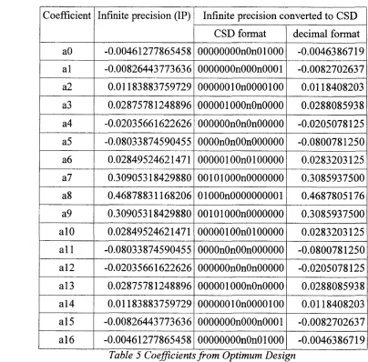
3.8 COMPARISON OF OPTIMUM SOLUTION WITH CSD CONVERSION ...54
3.9 CONCLUSION... 76
CHAPTER 4. 1-D RECURSIVE FILTER DESIGN... 77
4.1 RECURSIVE FILTERS... 77
4.2 DETERMINING FILTER STABILITY... 78
4.3 RECURSIVE FILTER DESIGN EXAMPLE... 81
4.4 OPTIMUM GA POPULATION SIZE TEST... 83
4.5 CONCLUSION...86
CHAPTER 5. TWO-DIMENSIONAL FILTERS...87
5.1 INTRODUCTION...87
5.2 2-D FILTERS AS CASCADED 1-D FILTERS... 88
5.3 FIR DESIGN EXAMPLE... 90
5.4 RECURSIVE 2-D DESIGN EXAMPLE...95
5.5 2-D NON-RECURSIVE FILTER EXAMPLE COMPARISON... 103
5.6 CONCLUSION... 104
CHAPTER 6. COMMON SUBEXPRESSION ELIMINATION...106
6.1 INTRODUCTION... 106
6.3 HORIZONTAL SUB EXPRESSION ELIMINATION WITHIN A
COEFFICIENT... 106
6.4 VERTICAL SUB EXPRESSION ELIMINATION...107
6.5 HORIZONTAL SUB-EXPRESSION ELIMINATION ACROSS COEFFICIENTS... 108
6.6 GRAPHICAL TRANSFORMATION ... 109
6.6.1. IDENTIFICATION GRAPH... 109
6.7 SEARCH GRAPH... 114
6.8 EXAMPLE WALK THROUGH SEARCH GRAPH... 115
6.9 EXAMPLE ELIMINATION USING A GA...116
6.9.1. FITNESS FUNCTION... 116
6.10 EXAMPLE... 117
6.11 APPLICATION TO PREVIOUS RESULTS...119
6.12SUMMARY OF APPLICATION TO PREVIOUS RESULTS... 126
6.13 CONCLUSION...126
CHAPTER 7. FUTURE WORK... 127
7.1 1-D RECURSIVE FILTERS... 127
7.2 2-D FILTERS... 127
7.3 COMMON SUB-EXPRESSION ELIMINATION...127
REFERENCES... 129
APPENDIX A SOURCE CODE... 134
APPENDIX B DEFINITIONS... 164
List of Tables
Table 1 GA Example: Initial Population... 16
Table 2 GA Example: S econ d Population...16
Table 3 Conversion Table for CSD Length L=7... 44
Table 4 Genetic Algorithm Param eters...46
Table 5 Coefficients from Optimum D esign ...48
Table 6 Coefficients for Filter from [36]... 51
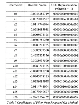
Table 7 Coefficients of Filter from Proposed GA Method... 53
Table 8 Comparison Summary... 53
Table 9 Infinite Precision C oefficients... 57
Table 10 Coefficients with a Maximum of 6 Non-Zero Digits... 58
Table 11 Coefficients with a Maximum of 5 Non-Zero Digits... 60
Table 12 Coefficients with a Maximum of 4 Non-Zero Digits... 64
Table 13 Coefficients with a Maximum of 3 Non-Zero Digits... 67
Table 14 Coefficients with a Maximum of 2 Non-Zero Digits... 69
Table 15 Coefficients with a Maximum of 1 Non-Zero Digit... 72
Table 16 Filter Square Error Relative to Filter with Optimum Infinite Precision Coefficients...75
Table 17 Coefficients of Exam ple R ecursive Filter... 82
Table 18 Optimum GA Population S iz e T est R esu lts... 84
Table 19. GA Param eters for 2-D FIR Exam ple...90
Table 21 Coefficients of F2 and G3 for 2-D FIR Exam ple... 94
Table 22 Coefficients of F3 and G3 for 2-D FIR Exam ple...95
Table 23 GA Param eters used for the 2-D Non-Recursive E x a m p le ...96
Table 24. Coefficients in Decimal and CSD Representation (where n = -1) for the 2-D Filter using C ascaded 2nd Order 1-D Filters... 98
Table 25. Coefficients in Decimal and CSD Representation (where n = -1) for 2-D Filter using C ascad ed 3rd Order 1-D Filters... 100
Table 26 Coefficients in Decimal and CSD Representation (where n = -1) for 2-D Filter using C ascad ed 4th Order 1-D F ilters... 102
Table 27. 1-D com ponent filter bias v a lu e s... 103
Table 28 Mean Square Error and Number of Additions Required for Coefficient Multiplication of Considered 2-D Filters... 104
Table 2 9 Coefficient Stacking... 111
Table 30 Properties of Vertices in ID Graph Exam ple...112
Table 31 Edge list E'id with E dge Properties... 113
Table 32 ID Graph Vertex Availability Table after (S6, S 3 ) Elimination...116
Table 33 CSD C oefficients... 118
Table 34 Coefficients with Eliminated S u b ex p ressio n s...119
Table 35 Eliminated Subexpression Labeling...119
Table 36 Eliminated Sub-E xpressions for Maximum 2 Non-Zero Digits...121
Table 37 Eliminated Sub-E xpressions for Maximum 3 Non-Zero Digits...122
Table 38 Eliminated su b ex p ressio n s for maximum 4 non-zero digits... 123
Table 4 0 Eliminated su bexpressions for maximum 6 non-zero digits... 125
List of Figures
Fig. 1.1 Shift-Add binary multiplication... 3
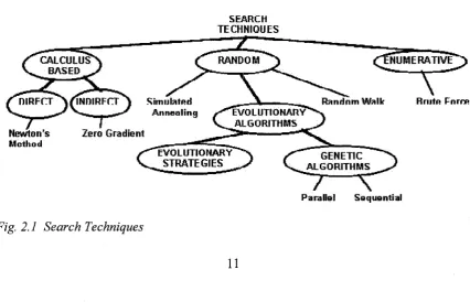
Fig. 2.1 Search T echniques... 11
Fig. 2.2 Sim ple Genetic Algorithm...12
Fig. 2.3 Sim ple Three Operator Genetic Algorithm ...13
Fig. 2.4 Single Point C rossover...15
Fig. 2.5 Uniform C rossover...26
Fig. 3.1 Invalid CSD C rossover...38
Fig. 3.2 Invalid CSD Mutation...39
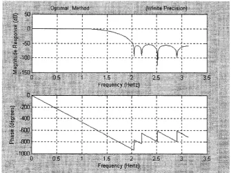
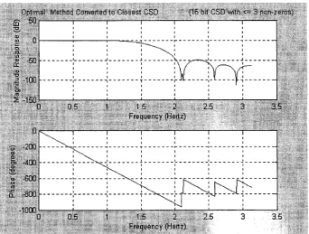
Fig. 3.3 Unlikely Mating Partners...4 0 Fig. 3.4 Impossible Mating Partners... 4 0 Fig. 3.5 R e sp o n se of Optimal D esign using IP C oefficients...4 7 Fig. 3.6 R e sp o n se of Optimal D esign Converted to CSD C o e ffic ie n ts... 4 9 Fig. 3.7 R e sp o n se o f Filter from [36]... 50
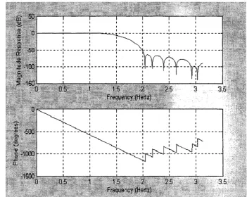
Fig. 3.8 R e sp o n se of design by proposed new m ethod...52
Fig. 3.9 R e sp o n se using Infinite Precision oefficients... 55
Fig. 3.10. R esp o n se of Filter with CSD Coefficients Converted from IP with a Maximum of 6 Non-Zero Digits... 56
Fig. 3.11 R esp o n se of Filter with CSD Coefficients D esign ed by GA with Maximum 6 Non-Zero Digits...59
Fig. 3 .1 3 R e sp o n se of filter with CSD Coefficients D esigned by proposed GA
method with a Maximum 5 of Non-Zero Digits... 62
Fig. 3.14 R e sp o n se of filter with CSD coefficients converted from IP with
maximum 4 non-zero digits... 63
Fig. 3.15 R e sp o n se of filter with CSD coefficients design ed by GA with
maximum 4 non-zero digit...65
Fig. 3.16 R e sp o n se of Filter with CSD Coefficients Converted from IP with a
Maximum of 3 Non-Zero Digits...66
Fig. 3 .1 7 R e sp o n se of the Filter with CSD coefficients D esign ed by GA with a
Maximum 3 Non-Zero Digits... 68
Fig. 3.18 R e sp o n se of the Filter with CSD Coefficients Converted from IP with a
maximum of 2 Non-Zero Digits...70
Fig. 3.19 R e sp o n se of the Filter with CSD Coefficients D esigned by GA with a
Maximum 2 Non-Zero Digits... 71
Fig. 3.20 CSD Coefficients Converted from IP with a Maximum of 1 non-zero
digit...73
Fig. 3.21 R e sp o n se of the Filter with CSD Coefficients D esign ed by GA with a
Maximum of 1 Non-Zero Digit...74
Fig. 4.1 Optimum Penalty Factor Determination... 80
Fig. 4 .2 z-P lan e Plot of the P o les (X) and Zeros (O) of the Exam ple
Non-R ecursive Filter...83
Fig. 4 .3 Optimum GA Population S iz e T est R esults... 85
Fig. 5.2 Target R e sp o n se ...91
Fig. 5.3 High Throughput Filter R e sp o n se ...91
Fig. 5.4 Target R esp o n se Error...92
Fig. 5.5. Desired Magnitude R e sp o n se of the 2-D Filter... 96
Fig. 5.6. Amplitude R e sp o n se of the 2-D Filter using C ascad ed 2nd order 1-D Filters with CSD C oefficients...97
Fig. 5.7 Amplitude R e sp o n se of the 2-D Filter using C ascad ed 3rd Order 1-D filters with CSD C oefficients... 99
Fig. 5.8 Amplitude resp o n se of the 2-D filter using ca sca d ed 4th order 1-D filters with C SD coefficients...101
Fig. 6.1 ID Graph with Only V ertices... 112
Fig. 6 .2 Partial ID Graph G'id... 113
Fig. 6 .3 Completed ID Graph Gid... 114
List of Abbreviations
0 Filter Zero
1-D One-dimension
2-D Two-dimensions
Bit limited Non-zero-bit Limited
CSD Canonical (or Canonic) Signed Digit
DSP Digital Signal Processing
E Set of Graph Edges
G Graph
GA Genetic Algorithm
ID Identification
IP Infinite Precision
LMS Least mean Square
MINIMAX Minimize the Maximum Error
N-D N-dimensions
SVD Singular Value Decomposition
TSP Traveling Salesman Problem
V Set of Graph Vertices
CHAPTER 1. INTRODUCTION
Digital Signal Processing (DSP) is a field of engineering that deals with the processing,
enhancement, and extraction of information for discrete time data. DSP has been applied
in the areas of radar signal processing, speech processing, communication, biomedical
image processing, and computer vision. Increasingly, DSP algorithms and devices are
being found in consumer products such as home theatre , music players, cell phones, etc.
An important area of DSP is digital filtering. It is a computational process, which
transforms a signal represented by an input array of numbers to another signal
represented by an output array of numbers, in order to alter the signal response
characteristic according to some prescribed specification.
Digital filters can be applied in one-dimension (1-D), two-dimensions (2-D), and in
general N-dimensions (N-D) and can be implemented on a general-purpose computer or
special-purpose hardware. The throughput of a digital filter is the rate at which an input
array can be transformed into a corresponding output array. For many applications a high
throughput will be required.
A 1-D recursive digital filter can be characterized by its difference equation (1.1)
N M
y i n T )~'Zj aix ( r i T - i T ) - ' Y J b , y { n T - i T ) (1.1)
( = 0 i = 1
a (i ) z 1
HI \ - A { z ) n n
H{z)
„
~
5 ( z ) (1.2)X b { i ) z ‘ i= 0
f o r sta b ility B ( z ) ^ 0 a n d | z | ^ l
output signal, n is a sequential sample number, T is the sample period and a„ bj are the
filter coefficients [1]. The magnitude and phase of the filter at a particular frequency w
is given by the transfer function when z = e J“T.
Filter design is the process determining the coefficient a.’s and bfs of the transfer
function such that the magnitude or phase of the frequency spectrum of the designed filter
approximates some desired response. Without loss of generality we assume M=N.
The filtering operation is performed according to the difference equation (1.1). Present
and past input and past output samples are multiplied by the filter coefficient a/s and bi's.
These products are summed to arrive at the output sample. The maximum speed at which
this operation can proceed is dominated by the time needed for multiplying the samples
by the filter coefficients. Decreasing the time needed for this multiplication will improve
the speed of the filter thus yielding higher throughput.
Binary multiplication is performed by a shift and add operation. The multiplier is
repeatedly shifted one or more bit positions and added to a partial product according to
( 10 1! ) • ( 10 10)
1 0 1 1
0 0 0 0
1 0 1 1
0 0 0 0
0 1 1 0 1 1 1
Fig. 1.1 Shift-Add binary multiplication
While shift operations execute quickly, additions are slower and comprise the bulk of
the multiplication time. Since an addition is required only when a 1 bit occurs in the
multiplicand, a multiplicand with fewer 1 bits will take less time to be multiplied than a
multiplicand with more 1 bits.
When performing a filtering operation the multiplier is chosen to be the input or output
sample and the multiplicand is one of the filter coefficients. Filters designed to have
coefficients comprising a small number of binary 1 digits are able to execute faster than
filters having coefficients comprising more binary 1 digits.
1.1 Canonical Signed Digit Number System
A common method [2]-[6] method for decreasing the number of binary 1 digits and
hence reducing the number of additions required during multiplication is to use the
Canonical Signed Digit (CSD) number system which inherently has a large number of
zero digits. It is based on the signed digit number systems [7] which allows individual
digits to have a sign as well as a value.
Generally the digits of these number systems are chosen as shown in (1.3) and can have
any base. As a replacement of the binary system for high speed multiplication, the ternary
number system where r = 2 is used. This allows the digits to have values of 0, 1 or -1.
Typically the -1 digit may be written as
I
or as the letter n (for negative 1). Here, theI
form will be used for clarity in equations, while the simpler n form will be used for long
compilations of CSD numbers.
In this number system, the sign and value of the overall number is determined by the
weighted sum of the signed digits as shown in (1.4).
N - 1
value = d 0d ]d 2 —, d N_\ = '^J d jx2 ~ ‘
i = 0
In multiplication, the shift and add operation of the binary number system is extended
to include subtraction for the case when a digit has a value of -1. Subtraction and addition
are comparable in terms of speed of execution so allowing -1 digits does not hinder
multiplication time yet the extra freedom offers a great potential to increase the number
of zero digits used to represent a given value.
The signed-digit number system is a redundant number system, since a given value
may be represented by more than one sequence of digits. For example,
0.01 = 1 X2~2 = .25 and 0. l I = l x 2 1- l x 2 “2= - . 2 5 are two different
However, for any given value with two or more redundant representations there will be
only one representation where the A-digit signed-digit number follows the constraint of
(1.5).
d nXd„+i = 0 for 0 < n < N — 2 (1.5)
Such a number is said to be the canonical form of the signed-digit number or simply
the CSD form. Following from (1.5) is the property that the number has no adjacent non
zero digits.
Another property of the CSD form is that it has the fewest number of non-zero digits
among the redundant forms. An N bit number in CSD format is able to uniquely express
every value of an N bit binary number but it will never have more (N+l)/2 non-zero bits.
This makes it a very desirable form for high throughput filtering.
1.2 Limiting Non-Zero Bits in Coefficients
A method of further reducing the number of non-zero digits in a coefficient is to simply
place an arbitrary limit on the the number of such digits allowed. Unfortunately, this
reduces the available values in the number system resulting in a loss of granularity in
coefficient choice thus ultimately limiting the quality of the filters which can be designed.
However, using appropriate design methods, good filters can still be designed.
For example, the designer can opt to allow no more than 3 non-zero digits within a 16
digit CSD coefficient. Such non-zero-bit limited (bit limited) CSD numbers are still
For example, the CSD number represented by 0 1 0 1 0 1 0 1 0 0 0 0 0 0 0 0 0 would not
be allowed if we were to set a non-zero bit limit of 3. Since this uniquely represents the
value -0.3359375, such a value would not be available. The closest value that could be
represented would be -0.328125 having a representation of OOlOlOTOOOOOOOOO
which, in this case, exhibits an approximate 2.3% error from the desired value.
Coefficients in this bit-limited format are guaranteed not to have more than the given
limit of non-zero digits making them well suited as operands in high speed multiplication.
However, filter designs become more difficult with fewer coefficient values to choose
from.
1.3 Survey of Filter Design Methodologies with CSD Coefficients
Several design methodologies have been used for designing CSD Coefficient Filters.
1.3.1. Conversion
Simply designing a filter using infinite precision numbers and converting each of the
filter's coefficients to bit-limited CSD numbers is problematic at best. Due to the poor
granularity of bit-limited CSD numbers, each conversion could introduce a fair amount of
error. It is likely that the accumulated errors of all coefficients will detrimentally effect
the filter's response. In addition, for recursive filters, a formerly stable filter may become
1.3.2. Algebraic Design
Designing a filter completely within a bit-limited CSD number system using direct
algebraic filter synthesis is not possible. Bit-limited CSD number systems are not closed
under normal arithmetic operations such as addition or multiplication. For example, the
sum o f two bit limited CSD numbers may have more non-zero digits than the limit allows
placing it outside the number system. Thus no bit-limited CSD algebra exists within
which direct filter synthesis calculations can be performed.
1.3.3. Search and Optimization
Some form of search and optimization is often used to design these filters. Standard
optimization algorithms, such as hill climbing, will get trapped in a local maximum of the
multimodal search space of a filter design.
Integer programming has been used successfully for low order filters but it tends to
become impractical for higher order filters [5] due to the search space becoming
extremely large.
Simulated annealing has been shown to be effective in filter design but it suffers from
high computational costs [8].
A computationally efficient method which has a parallel searching capability is the
Genetic Algorithm [9]. It can handle large search spaces and has been shown to work
To date though, this method has been hampered by its inability to efficiently handle the
CSD constraints. All solutions have introduced some form of random search into an
otherwise robust search method. The resulting search methods are no longer pure Genetic
Algorithms but hybrids of random search and GA principles.
In this dissertation a method is presented for applying a GA to this problem with a new
coding technique that makes it possible to utilize the full potential of the genetic
algorithm. Many examples and comparisons are included to demonstrate the effectiveness
of this method.
1.4 Common Sub-expression Elimination
The throughput of the implementation of CSD-coefficient filters is determined by
the number of additions required to implement the coefficient multiplication using a
shift/add procedure. The number of these additions can be reduced by avoiding redundant
calculations through the use of common sub-expression elimination.
In this dissertation a method is presented for transforming this problem into one similar
to the well understood Traveling Salesman problem [9]. An example using a standard GA
is included to demonstrate the effectiveness of this method.
1.5 Organization of this Dissertation
This dissertation covers several topics. Chapter 1 is a general introduction. Chapter 2
continues with a detailed examination of Genetic Algorithms. Chapter 3 looks at 1-D
filter non-recursive design and Chapter 4 extends this to recursive filter design. Chapter
CHAPTER 2. GENETIC ALGORITHMS
2.1 Introduction
This chapter examines the basic operation of Genetic Algorithms including the
essential operations of selection, crossover and mutation. The theoretical foundations are
reviewed including the fundamental theorem of Genetic Algorithms, the building block
theorem and implicit parallelism. Advancements and refinements to the basic operators,
as well as techniques for managing GA difficulties, are examined.
2.2 Origin and Operation
Genetic algorithms are a class of computational methods that are modeled on the
mechanisms of natural evolutionary genetics. The first rigorous study of GA principles
was reported by John Holland in his book Adaptation in Natural and Artificial Systems
published in 1975 [10]. This work has been subsequently extended by many others. They
utilize methods that are similar to the methods found in natural selection to work. These
methods operate on a population of problem solutions in an effort to find the fittest
individual. It is hoped that this fittest individual is at or close to the optimal solution
The technique is based on the principles of survival of the fittest. Individuals in a
population must compete with each other for a limited number of resources and
ultimately for survival. The most successful individuals will more likely survive and thus
mate. The less successful individuals will be less likely to survive and thus will produce
will more likely inherit genes from the successful individuals than from the unsuccessful
ones.
Genetic algorithms borrow heavily from this natural evolutionary process to allow
solutions to real world problems to evolve over many succeeding generations. Therefore,
in order to artificially use the mechanisms of natural selection on a search and
optimization problem, it is necessary to formulate the problem in line with that observed
in nature. The solution to the problem must be expressed as a character string called a
chromosome and there must also be a fitness function that can be applied to this string to
determine the individual’s fitness.
For example, in the design of a bridge the chromosomes may represent the size and
weight of certain beams. The fitness function would calculate the strength to weight ratio
of a bridge built with these beams. The GA would then be searching for the beams with
the highest strength to weight ratio.
Within a population of individual solutions to a problem there are more fit and less fit
solutions. Individuals are chosen from this population for mating depending upon their
fitness score. Two chosen individuals are mated by cutting and splicing their
chromosomes to form a new chromosome. The offspring will thus inherit features from
both parents. In this way the good characteristics of a population are transferred to each
succeeding population while the bad characteristics are not. This results in the most
promising areas of the search space being explored. If the problem has been coded into
The GA is robust since the only requirement for applying it to a particular problem is
that the solution can be expressed as a chromosome and there exists a fitness function to
evaluate this chromosome’s fitness. No other information about the problem is needed.
This means that a GA can be applied to a wide variety of problems including some of
those where there are no other solution techniques.
A GA does not actually find a solution to a problem but instead creates new and better
solutions based on existing solutions. Fortunately, the coding of a solution into a string as
required by the GA allows initial solutions to be randomly generated. While GAs are not
guaranteed to find the global optimum, they are good at finding good solutions in a
reasonable amount of time.
2.3 Classes of Search Techniques
Genetic algorithms are a type of optimization search technique. Search techniques in
general, as illustrated in Fig. 2.1, can be grouped into three broad classes [10] calculus
based, enumerative and random search.
SEARCH
TECHNIQUES
CALCULUS BASED _
NUMERATIVE RANDOM
R a n d o m W alk niR F C T
EVOLUTIONARY ALGORITHMS
Zero Gradient Newton’s
M eth o d
EVOLUTIONARY
STRATEGIES ALGORITHM SGENETIC
P a ra lle l S e q u e n tia l
Calculus based methods include direct and indirect. Indirect is the search for the peaks
of maxima by finding zero of the gradient. Direct techniques are those such as Newton’s
method. Random methods include simulated annealing, evolutionary strategies, genetic
algorithms and the simple random walk through the search space. Enumerative methods
are the brute force methods where all the solutions in the whole search space are
generated.
BEGIN SIMPLE GENETIC ALGORITHM Randomly generate initial population
Compute the fitness of each individual in the population WHILE (NOT finished) DO
// produce new generation FOR (population_size / 2) DO
Reproduction:
- Copy two parent individuals randomly selected from current generation using probability biased to favor the fittest
- Mate these copies by randomly splitting and recombining them to form two new offspring
Crossover:
- Remove the two original parents from current generation - Place the two offspring into new generation
END FOR
Designate new generation to be current generation Randomly change some randomly selected individuals
Mutation:
Compute the fitness of each individual
IF (population has converged) THEN finished
END IF END WHILE
END GENETIC SIMPLE ALGORITHM
Fig. 2.2 Simple Genetic Algorithm
The basic simple genetic algorithm, as described by Goldberg [10], is shown in Fig.
2.2. It is composed of three operators: reproduction, crossover, and mutation. These are
the problem. The problem must have a fitness function that can be applied to each
solution to determine its merit or fitness. Applying the operators to a population results in
a new population with hopefully increased average fitness as well as an increase in the
fitness of the fittest individual. This process is repeated until there is no further fitness
increase at which time the solution is said to have converged. The cycle is shown more
graphically in Fig. 2.3.
I V f u t a T i o t w . ( ]
T j
x
j*
-Fig. 2.3 Simple Three Operator Genetic Algorithm
2.4 Problem Coding
The problem solution must be encoded in a form suitable for use with the reproduction,
crossover, and mutation operators. The solution must be configured as a string of
characters called a chromosome after its biological analogue. The characters, also called
genes, may be taken from any fixed alphabet that may be used to represent the problem.
Early work [11] suggested that a longer string is superior to a shorter string so a low
cardinality alphabet is superior to a higher one. Later work however [12],[13], shows that
some problems do better with a higher cardinality7 chromosome. The lowest cardinality
code problems. In biology, chromosomes are made of strings of four different proteins so
the biological alphabet has a cardinality of four.
2.4.1. Fitness Function
The problem must also have an objective or fitness function that takes a solution
chromosome and returns a value that represents a figure of merit for this solution. A
higher figure of merit indicates a superior or fitter solution.
The genetic algorithm works on a population of chromosome strings each of which
represent a solution to the problem. To begin, an initial population of solution strings is
chosen by some method such as simple random choice. This population is applied to the
objective function and each solution is assigned a fitness value. The population is then
subjected to the three operators of the genetic algorithm.
2.4.2. Reproduction
Reproduction is the process of randomly selecting chromosome strings biased by their
fitness value and making new chromosome strings out of them. A chromosome string
with a higher fitness value will have a higher probability of being chosen for
reproduction. This is analogous to the natural selection process whereby an organism that
is more fit has a higher chance of surviving to reproduce.
Implementing a biased random selection in algorithmic form can be accomplished in
Instead each is sized in proportion to its corresponding chromosome's fitness. When the
wheel is spun the chromosome string with the highest fitness will have the greatest
possibility of being chosen. An entire population is chosen this way. Some may be
chosen more than once. This method was used throughout this dissertation.
These selected individuals are used to create new strings through the crossover
operation. In single point crossover, as shown in Fig. 2.4, a crossover point is chosen at a
random position between 1 and the string length-1 which in this case is the third position.
Two new chromosome strings are now created by dividing the initial chromosome strings
into two sections each at the crossover point and appending the first half of the first
chromosome string to the second half of the second chromosome string and vice versa.
F i r s t p a r e n t = A B C | D E F G s u b s t r i n g l = A B C
S e c o n d p a r e n t = a b c | d e f g s u b s t r i n g 2 = d e f g
o f f s p r i n g l = s u b s t r i n g l + s u b s t r i n g 2 = A B C d e f g
o f f s p r i n g 2 = s u b s t r i n g 2 + s u b s t r i n g l = a b c D E F G
Fig. 2.4 Single Point Crossover
The mutation operator is now applied to the population. This operator applies a random
alteration to the value of a chromosome string position. This alteration occurs with very
small probability so that the likelihood of a bit actually mutating is very small. Mutation
is necessary to replace genetic information that may have been lost or may never have
existed in the original population.
2.5 Example Problem
The simplicity and power of genetic algorithms can best be demonstrated with the step
simple that it was solved by hand by Goldberg [9] using nothing more than a coin to
generate random numbers. Yet even with this simplicity the improvements possible in
only a single generation are readily apparent.
The problem goal is to maximize the function f(x)=x2 where x is permitted to vary
between 1 and 31 which is coded as a 5 bit binary number. To keep things manageable it
is run with a population of only 4 individuals.
String Num ber
Initial Population (Chromosome)
x Value (as Integer) Objective Function Value f(x)=x2 Probabi lit y of Selection
Expected Count
Actual Count (From Roulette W heel) 1 0 1 1 0 1 13 169 0.14 0.58 1
2 1 1 0 0 0 24 576 0.49 1.97 2
3 0 1 0 0 0 8 64 0.06 0.22 0
4 1 0 0 1 1 19 361 0.31 1.23 1
Sum 1170 1.00 4.00 4.0
Average 293 0.25 1.00 1.0
M aximum 576 0.49 1 97 2 0
Table 1 GA Example: Initial Population
String Number Mating Pool After Reproduction Mate (Randomly Selected) Crossover Site New Population
x Value (Integer)
Fjx} X2
1 0 1 1 0 1 2 4 0 1 1 0 0 12 144
2 1 1 0 0 0 1 4 1 1 0 0 1 25 625
3 11 0 0 0 4 2 1 1 0 1 1 27 729
4 10 0 1 1 3 2 1 0 0 0 0 16 256
Sum 1754
Average 439
Maximum 729
In the initial population the average fitness is 293 and the best individual fitness is 576.
After one generation the average fitness has increased to 439 and the best individual
fitness has increased to 729.
2.6 Analysis of the Simple Three Operator Genetic Algorithm
The previous section demonstrated the mechanics of the simple three operator genetic
algorithm. By mimicking nature, a procedure has been developed that seems to provide
useful results. However, to understand why it works requires a theoretical analysis.
This theoretical basis for the GA’s operation was first worked out by Holland [11] and
later embellished by Goldberg [9]. It provides a thorough, generalized analysis of the
operation of GA’s. This analysis is often called the schema theorem, but its real
importance is underscored by its other commonly used name: the fundamental theorem of
genetic algorithms.
2.6.1. Schemata
In order to analyze the workings of genetic algorithms it is necessary to have some
method of describing a subset of a string. A subset can be described using the similarity
template called a schema (in plural form they are called schemata). This is a string
composed of the letters of the given chromosome alphabet plus a special symbol, usually
*, that is used to indicate a don’t care position in the chromosome string. A schema can
if in every location a 1 in the schema matches a 1 in the chromosome string and a 0 in the
schema matches a 0 in the chromosome string and a * matches either.
For example, consider the case of a binary string of length 5. The schema * 1 0 1*
matches only the chromosome strings 01010, 01011, 11010 and 11011.
2.7 The Fundamental Theorem of Genetic Algorithms
The schemata theorem or the fundamental theorem of genetic algorithms is one of the
most important properties related to genetic algorithms. In order to analyze the operation
of genetic algorithms it is necessary to be able to count the schemata present within a
population of strings and determine which grow and which decay during each generation.
This is done by considering the affect of reproduction, crossover and mutation on a
particular schema. The objective is to quantifying the GA’s simultaneous manipulation of
a very large number of schemata.
2.7.1. Notation
In this analysis it is considered, without loss of generality, that strings are composed of
characters from the binary alphabet V= {0,1}. For notational purposes strings will be
referred to by capital letters and individual characters in the string by lower case letters.
These individual characters may be subscripted by their position in the string as in
5,=SiS2s3S4. Populations of individual strings will be denoted as P„ j = 1, 2,. . ,,n . A
population existing at a time or generation t and will be denoted as P(t), where the
In order to describe the schema contained in individual strings and populations the
three letter alphabet V+ = {0,1,*} will be used. The additional character * is used as a
don’t care or wild card symbol which will match either a 0 or a 1 at any particular string
position.
For a string of length / there are 3 ' schemata which are defined over it. In general, for
an alphabet of cardinality j there are (j + 1) ' schemata.
The order of a schema is denoted by O (H ) , and is the number of fixed (as opposed to
wild card) positions that it has. For example, a schema of length 5 and order 3 is 1 1 1 * *
A schema H will also have a defining length denoted by 6 ( H ) . This is the distance
between the first and last fixed string position. For example the schema 1 * 1 * * has a
defining length 5 ( H ) —2 because the first fixed position is 1 and the last fixed position
is 3 and 3-1 = 2 . Similarly, the schema * 1 * * * * would have a defining length of
<5(/F) = 2 —2 = 0 .
2.7.2. Analysis of the Fundamental Theorem O f Genetic Algorithms
The previously discussed notation will be used to discuss the effect of reproduction on
the expected number of schemata in the population. Suppose at a given time t there are m
examples of a particular schema H contained within population A(t). This can be written
asm = m(h, t). During reproduction a string A gets selected for copying with a probability
replacement from the population Aft), there should be m(H, t + 1) representatives of the
schema H in the population at time t + 1 as given by (2.1).
m (H , t + \ ) = m ( H (2.1)
2 -i J i
If f { H ) is the average fitness of the strings representing schema H at time t and since
the average fitness of an entire population may be written as / = £ / , / « the reproductive
schemata growth equation may be written as:
m ( H J + \ ) = m ( H j ) ^ = P ~ (2.2)
This shows that a particular schema grows as the ratio of the average fitness of the
schemata to the average fitness of the population. Schemata with fitness values greater
than the population average will be present in greater numbers in the next generation
while schemata with fitness values lower than the population average will be present in
lesser numbers in the next generation. This operation is carried out with every schema in
a particular population A in parallel. All schemata in the population grow or decay
according to their schemata averages under the operation of reproduction. This simple
operation of reproduction on the strings in a given population results in many more
operations being performed on many more schemata.
Individual schema will increase or decrease in number from generation to generation
depending upon their fitness values. The exact rate of this growth or decay can be
remains above average by about c / with c a constant. The schema difference equation
can then be rewritten as in (2.3).
Starting at / = 0 , and assuming c is constant from generation to generation, (2.4) is
obtained:
This equation has the same form as the compound interest equation. It is a geometric
progression which shows that reproduction allocates exponentially increasing or
decreasing numbers of schemata. It can also be seen that for a schema that is above or
below average, reproduction will allocate exponentially increasing or exponentially
decreasing offspring in subsequent generations.
The reproduction operation ensures that subsequent generations will have exponentially
increasing numbers of schemata that are fit and exponentially decreasing numbers of
schemata that are not fit. This operation serves to concentrate the existing good solutions
while eliminating some of the less good solutions. It does nothing to find new and
possibly better solutions. This is the job of the crossover operator.
Crossover allows for a randomized exchange of information between strings. It creates
new strings while preserving the allocation strategy pursued by reproduction. The result
is an exponentially increasing or decreasing collections of particular schema throughout
the population.
(2.3)
During the operation of crossover some schema are more likely to survive than others.
For example, the schema * * * 1 0 * * can only be destroyed if the crossover point is
chosen so that it falls between the 1 and the zero at the 4* position. On the other hand the
schema * 1 * * * * 0 can be destroyed if the crossover point falls between the 1 and the 0
at any of positions 2, 3, 4, 5 or 6. The likelihood of survival is based on the defining
length of the schema and is given by the crossover survival probability p s .
The lower bound of the crossover survival probability P s can be calculated under
simple crossover as p s= \ —6 ( H) / ( l — l) since the schema is likely to be destroyed
whenever a crossover site within the defining length is selected from the l —l possible
sites. Since the crossover is itself performed by random choice with a probability P c at a
particular mating, the survival probability may be given by (2.5).
P s ^ - P c ' - J Z l (2-5)
As can be seen, this expression reduces to the previous expressions whenever Pc - 1 .
In order to calculate the number of a particular schema H expected in the next
generation under the combined effect of reproduction and crossover, the combined
expression in (2.6) is used.
6 ( H)
1 - P c " / - l (2.6)
/
schema H to survive, all of its fixed positions must survive. Therefore, a single character
of a schema survives with the probability 1- Pm . Since each of the mutations is
statistically independent, a particular schema survives when each of the o ( H) fixed
positions within the schema survives. Multiplying the survival probability 1— Pm by
itself o ( H ) times is the probability of surviving mutation as ( \ —p m)°^H\ Since the
probability Pm is very small (Pm« 1) this can be approximated as 1 - o ( H ) ( p m) .
Combining this with the previous expression gives the following relation describing the
number of copies of a particular schema that can expect to survive into the next
generation under all three operations of reproduction, crossover and recreation.
5 ( H )
* f ( H )
m ( H , t + \ ) > m ( H , t) 1 - Pc
1-1 ~ ° ( H ) p (2.7)
f
This shows that short, low order, above average schemata receive exponentially
increasing trials in subsequent generations. These schemata are often referred to as
building blocks and their exponentially increasing importance to the outcome of a GA is
often referred to as the building block theorem.
2.8 Implicit Parallelism
The results of the preceding analysis has been used to define a phenomenon called
implicit parallelism [9] that explains the power of GAs. Here a GA, with a population of
n, processes n chromosomes for each generation. During these n calculations the GA is
2.9 Advanced Techniques
The simple genetic algorithm, as discussed so far, is the basic starting point for all
genetic algorithms. Much research has gone into extending and improving the algorithm.
Many of these advanced techniques have come to be used routinely.
2.9.1. Crossover Techniques
The simple GA performs crossover by making a single cut at the same location in each
of the two parent chromosomes. This cut occurs somewhere between the first gene and
the last gene. The cut sections are then exchanged to form two offspring. This method is
somewhat simplistic and tends to destroy the building blocks that contain widely spaced
genes. For this reason researchers have devised many new crossover techniques often
using more than one cut point.
The effectiveness of multiple-point crossover was investigated and it was found [14]
that while 2-point crossover gives an improvement, adding further crossover points
reduces the performance of the GA. As additional crossover points are added, the search
becomes more random because building blocks are more likely to be disrupted. The
problem space is searched more thoroughly at the expense of greatly increased search
time. In the extreme, the search simply becomes a random search.
2 .9 .l.a ) 2-Point Crossover
2-point crossover has chromosomes arranged in loops by joining their ends together.
be seen that 1-point crossover is just a special case of the more general 2-point crossover
where one of the cut points is fixed as falling between the last and first position. This
would account for the increased performance seen when 2-point crossover is used. It is no
more disruptive than 1-point crossover since they both have 2 cut points and 2-point
crossover does not always destroy building blocks with widely spaced genes as is the
case for 1-point crossover. That is, a chromosome treated as a loop with no beginning and
no end can contain more building blocks, since they are able to wrap around at the end of
the string. It is generally considered that 2-point crossover is superior to 1-point
crossover.
2.9.1.b) Uniform Crossover
Another form of crossover is the n-point uniform crossover where the number of points
n varies dynamically with each mating. In this method, a randomly generated crossover
mask is used to determine which genes of an offspring come from which parent. Each
gene in the first offspring is created by copying the corresponding gene from one or the
other parent according to the crossover mask. Where there is a 1 in the mask, the gene is
copied from the first parent, and where there is a 0 in the mask, the gene is copied from
the second parent. The process is repeated with the parents exchanged to produce the
second offspring. A new crossover mask is randomly generated for each pair of parents.
Offspring, therefore, contain a mixture of genes from each parent. The number of
effective crossing points, while not fixed, will average L/2 (where L is the length of the
For example, suppose we let the first parent be an arbitrary 10-bit binary string
represented by the sequence ABCDEFG where A represents the most significant bit and
G the least significant bit and similarly we let the second parent be represented by
abcdefg then they would mate using uniform crossover as follows:
1. A random crossover mask is chosen, ( e.g. 0011101001)
2. Wherever the mask has a 1, choose the corresponding character from the first parent
3. Wherever the mask has a 0, choose the corresponding character from the second parent
4. The resulting offspring is combined as shown in Fig. 2.5
5. Reverse parents and repeat steps 2, 3, & 4 yielding the second offspring (A B c d e F g)
P a r e n t A B C D E F G a b c d e f G
M a s k 0 0 1 1 1 0 1 0 0 1 1 1 0 1
R e s u l t - - C D E - G a b - - - f
-C o m b i n e d O f f s p r i n g a b C D E f G
Fig. 2.5 Uniform C rossover
2.9.2.Crossover Comparisons
Research on the different methods of crossover [15] has shown that uniform crossover
produces long defining length schema which are less likely to be disrupted than those
produced by 2-point crossover. But while the short defining length schemata of 2-point
crossover are more likely to be disrupted, the overall amount of schemata disruption is
Under 2-point crossover the defining length, and not the order of the schemata,
determines the likelihood of its disruption. Under a uniform crossover, the likelihood of
disruption of a given schema is based only on its order and not its defining length. This
means that under a uniform crossover, the ordering of genes within a chromosome is
completely irrelevant and it eliminates the need for re-ordering operators such as
inversion (see Section 2.9.6 Inversion and Reordering, on page 30). Also, since the
positioning of genes is immaterial there is no need to worry about coding the
chromosome in such a fashion so as to create good building blocks.
In another study [16] an extensive comparison of 1-point, 2-point, multi-point and
uniform crossover operators was performed. Theoretical analysis was performed in terms
of positional and distributional bias on several problems. The findings indicated that there
was only about a 20% difference in speed between the slowest and fastest techniques.
From these results the choice of a crossover operator would seem to be relatively
unimportant.
Other analysis [17] of crossover has shown that due to reduced productivity, 2-point
crossover will perform poorly when the population has largely converged. Productivity is
the ability of a crossover operator to produce new chromosomes that are different,
thereby sampling new points in the search space. If two similar chromosomes undergo 2-
point crossover, then the exchanged segm ents are likely to be identical causing the
offspring to be identical to their parents. Under uniform crossover, this is less likely to
Many problems benefit when a few parents are not crossed over at all but passed on
intact. Many algorithms apply a high probability crossover rate which performs crossover
most of the time but once in a while randomly passes the parents through with performing
crossover.
Another operator called elitism takes the most fit individual and automatically passes it
through, intact, to the next generation. This is done to make sure the best solution so far
is not lost.
2.9.3. Other Crossover Techniques
A new 2-point crossover operator has been reported [18] where the offspring are
checked after crossover and if they are found to be identical to their parents then
crossover is repeated using two new crossover points. When tested, this new operator was
found to perform slightly better than uniform crossover. This new 2-point crossover is
best only when there is a large population, and that for small populations uniform
crossover is best due to the increased disruption that it causes.
Several methods have been described [19]-[22] that vary the probability of crossover
occurring at a particular string position. The crossover probabilities themselves become
part of the chromosome so that the GA dynamically adjusts the sites that should be
favored for crossover. With the crossover probabilities included as part of the
chromosome, they are crossed over and passed on to descendants allowing the GA to
2.9.4.Crossover Conclusion
Although the crossover method used has only a modest affect on the overall
performance of a GA, one of the top ranked crossovers is uniform crossover. As well,
under uniform crossover the ordering of genes within a chromosome is completely
irrelevant. For these reason all GA's used in the examples in this dissertation will employ
elitism and uniform crossover.
2.9.5. Mutation
Normally, mutation occurs with low probability and functions as a background operator
[14]. It is included to allow for the searching space that may otherwise be precluded by
the converging chromosomes as the genetic information is discarded during crossover.
The exact amount of mutation necessary is somewhat open to debate. Too little mutation
and useful schemata that are not currently in the population can never be found while too
much mutation will cause the GA to degenerate into a random search.
A study [23] to determine the optimum parameters for GAs found that mutation plays a
larger role than previously thought. Another study [24] compared crossover and mutation
and found that each operator contained characteristics not found in the other but that each
is simply a form of a more general exploration operator that modifies schemata based on
available information. As the population converges, mutation plays an increasingly
Although it has a low probability of use and it is sometimes seen as nothing more than
a background operation, mutation plays a very important part in a GA solution. Changes
in the mutation rate will affect the performance more than the changes to the crossover
parameters [23]. However adjusting for the optimum mutation rate is difficult as long as
extremes are avoided. There is a fairly broad range of values that seem to work well in
most situations.
2.9.6. Inversion and Reordering
For a GA to work effectively, the building block theorem requires that the genes be
arranged in a particular order in the chromosome. To accomplish this, techniques for
reordering the positions of genes have been developed. One of these techniques is
inversion [11] which reverses the order of genes between two randomly chosen positions
within the chromosome. To keep track of a gene's position within the chromosome some
auxiliary positioning information must be maintained with each chromosome. Gene
reordering is an attempt to create chromosome codings with better evolutionary potential
[9].
When reordering is used, the search space is greatly expanded, since the GA is
searching for a solution to the original problem and simultaneously searching for the
optimum gene ordering. The extra search time spent on ordering might be better spent on
When a uniform crossover is used, the ordering of genes is irrelevant so reordering
would have absolutely no effect. Since in this dissertation uniform crossover will be used
exclusively, reordering will not be performed.
2.9.7. Deception
The building block principle states that over succeeding generations there will be an
increase in the number of chromosomes containing schemata that are also found in the
global optimum until eventually these schemata will crossover into a single individual
and the global optimum will be found. But on certain GA deceptive problems, this does
not occur and schemata that are not in the global optimum increase in numbers faster than
those that are.
This phenomenon has been studied in depth by many [9],[26],[27] and it has been
shown that the number of chromosomes containing a particular schema will increase if
the schema’s fitness is higher than the average fitness of all schemata in the population.
The difficulty arises if the average fitness of schemata which are not contained in the
global optimum is greater than the average fitness of those which are. This class of
problem is deemed to be deceptive. A GA will usually, but not always, have difficulty
solving a deceptive problem.
A problem that is deceptive with one chromosome coding format may not be with a
different format. Therefore the coding format can be crucial to the success or failure of
2.9.8. Epistasis
A given gene’s contribution to the overall fitness of an individual may be conditional
on the value of other genes in the chromosome. Such a gene would be called epistatic. In
general, the amount of co-dependency among genes is termed epistasis and occurs in
nature on a regular basis. For example, bats have a gene that gives them their keen
hearing and another to make high pitched chirps. Either of these genes alone would not
increase a bat’s fitness but together they form a sonar system and have a major impact on
fitness.
The amount of epistasis which occurs can vary from none to severe. An example of a
problem with no epistasis is the counting of ones task where the task is to maximize the
number of 1 s in the binary string. In this case each gene (bit) either has a value of 1 and
contributes to the fitness or has a value of 0 and doesn’t. An example of moderate
epistasis is the plateau function where the fitness is 1 if all the bits in a chromosome are
set to 1, and zero otherwise. Here the genes do interact but only for the global optimum
when they all must be 1. Severe epistasis is where the genes interact in numerous and
complex ways. An example of this would be a scheduling problem where the availability

![Fig. 3.7 Response o f Filter from [36]](https://thumb-us.123doks.com/thumbv2/123dok_us/1482613.1181410/69.610.73.509.109.770/fig-response-o-f-filter-from.webp)
![Table 6 Coefficients for Filter from [36]](https://thumb-us.123doks.com/thumbv2/123dok_us/1482613.1181410/70.610.159.476.86.482/table-coefficients-for-filter-from.webp)