A Comparative Study of Document Representation Methods

(1)

University of Windsor University of Windsor

Scholarship at UWindsor

Electronic Theses and Dissertations Theses, Dissertations, and Major Papers

1-1-2019

A Comparative Study of Document Representation Methods

Ziyang Tian

University of Windsor

Follow this and additional works at: https://scholar.uwindsor.ca/etd

Recommended Citation Recommended Citation

Tian, Ziyang, "A Comparative Study of Document Representation Methods" (2019). Electronic Theses and Dissertations. 8183.

https://scholar.uwindsor.ca/etd/8183

(2)

A Comparative Study of Document

Representation Methods

By

Ziyang Tian

A Thesis

Submitted to the Faculty of Graduate Studies through the School of Computer Science in Partial Fulfillment of the Requirements for

the Degree of Master of Science at the University of Windsor

Windsor, Ontario, Canada

2019

c

(3)

A Comparative Study of Document Representation Methods

by

Ziyang Tian

APPROVED BY:

B. Shahrrava

Department of Electrical and Computer Engineering

A. Ngom

School of Computer Science

J. Lu, Advisor School of Computer Science

(4)

DECLARATION OF ORIGINALITY

I hereby certify that I am the sole author of this thesis and that no part of this

thesis has been published or submitted for publication.

I certify that, to the best of my knowledge, my thesis does not infringe upon

anyone’s copyright nor violate any proprietary rights and that any ideas, techniques,

quotations, or any other material from the work of other people included in my

thesis, published or otherwise, are fully acknowledged in accordance with the standard

referencing practices. Furthermore, to the extent that I have included copyrighted

material that surpasses the bounds of fair dealing within the meaning of the Canada

Copyright Act, I certify that I have obtained a written permission from the copyright

owner(s) to include such material(s) in my thesis and have included copies of such

copyright clearances to my appendix.

I declare that this is a true copy of my thesis, including any final revisions, as

approved by my thesis committee and the Graduate Studies office, and that this thesis

(5)

ABSTRACT

Document representation learning is crucial for downstream machine learning

tasks such as document classification. Recent neural network approaches such as

Doc2Vec and its variants are popular. Regarding its comparison with traditional

rep-resentation methods such as the TF-IDF method, the results are not very conclusive

due to several factors– Doc2vec has many hyper-parameters, resulting in performance

fluctuation; traditional methods have space to improve. More importantly, document

length and data size have impacts on the result. This thesis conducts a comparative

study of these methods, and propose to improve the TF-IDF weighting with mutual

information(MI). We find that Doc2vec works good only for short documents, and

only when the data size (the number of documents) is large. For long documents and

small data size, MI performs better. The experiments are conducted extensively on

11 data sets that are of a variety of combinations of document length and data size.

In addition, we study the relationship between TF-IDF and MI weighting. We

find that their correlation is high overall (Pearson correlation coefficient is over 0.9 on

all the data sets used in our thesis). For medium frequency words, the MI weighting

is always smaller than the TF-IDF weighting. However, for rare words and popular

words, MI diverges from TF-IDF greatly, and the weighting of MI is higher than

(6)

ACKNOWLEDGEMENTS

I would like to express my sincere appreciation to my supervisor Dr. Jianguo Lu,

for his constant guidance and encouragement during my whole Master’s period at the

University of Windsor. Without his valuable help, this thesis would not have been

possible.

I would also like to express my appreciation to my thesis committee members Dr.

Alioune Ngom and Dr. Behnam Shahrrava. Thank you all for your valuable guidance

and suggestions to this thesis.

Last but not least, I want to express my gratitude to my parents and my friends

(7)

TABLE OF CONTENTS

DECLARATION OF ORIGINALITY III

ABSTRACT IV

ACKNOWLEDGEMENTS V

LIST OF TABLES VIII

LIST OF FIGURES IX

1 Introduction 1

2 Review of the Literature 4

2.1 Na¨ıve Bayes[20] . . . 4

2.2 SVM(Support Vector Machine) with NB(Na¨ıve Bayes) features[21] . . 5

2.3 Character-level CNN[24] . . . 7

2.4 FastText[7] . . . 9

3 Traditional Methods For Document Representation 12 3.1 Term Frequency(TF) . . . 12

3.2 Term Frequency-Inverse Document Frequency . . . 15

3.3 Mutual Information Representation . . . 16

3.4 Comparing MI Representation with TF-IDF Representation . . . 19

3.4.1 Words that Occur Once . . . 20

3.4.2 Relationship with df . . . 24

3.4.3 Relationship with T F . . . 27

4 Neural Network Methods 33 4.1 Doc2vec - PV-DBOW . . . 33

4.2 Doc2Vec with Corruptions . . . 36

4.2.1 Doc2Vec PV-DM . . . 36

4.2.2 Doc2Vec with Corruption . . . 37

5 Experiments 40 5.1 Datasets . . . 40

5.1.1 Data Description . . . 41

5.1.2 Observation of Datasets . . . 43

5.2 Experimental Setup . . . 47

5.3 Comparison of MI and TF-IDF . . . 48

5.4 Compare of Neural Network Methods and the TF-IDF and MI . . . . 50

5.4.1 Hyper Parameters . . . 50

(8)

5.6 Impact of Shifting on MI . . . 58 5.6.1 What is Shifting? . . . 58 5.6.2 Experimental Results . . . 63

6 Conclusions 66

REFERENCES 68

(9)

LIST OF TABLES

1 Explanation of Symbols . . . 13

2 Example corpus of TF . . . 13

3 An example of document-word matrix for the corpus in Table 2. . . . 13

4 IDF of words in Table 2 . . . 15

5 Example of TF-IDF representation matrix . . . 16

6 Example of CT F, Di . . . 17

7 Example of MI representation matrix . . . 17

8 Pearson correlation coefficient between these two representations on the datasets used in our thesis. . . 19

9 The average of MI and TF-IDF when T F = CT F = df = 1. All the average of TF-IDF is greater than the average of the MI. . . 20

10 Detailed information of all datasets in this thesis. . . 40

11 Macro-F1 score of MI representation and TF-IDF representation on all datasets used in our thesis (Higher is better). Bold means better in that datasets. . . 48

12 P-value of significance test on the macro-F1 score between MI and TF-IDF results. Italic means no significant difference. . . 49

13 Experiments Records for TF, TF-IDF, MI, PV-DBOW and Doc2VecC on all datasets used in our thesis. . . 51

14 Number of data sets the different methods can give the best results. . 58

(10)

LIST OF FIGURES

1 Text classification system . . . 1

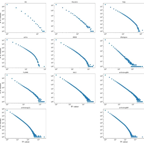
2 Distributions of TF values on all datasets used in this thesis. The

x-axis is the term frequency of the terms, and the y-x-axis is the times of

that term frequency appearance. Each dot is a term frequency, e.g., in

dataset AG, there are more than 106 _{terms with} _{T F} _{= 1 and nearly}

106 _with _{T F} _{= 2. . . .} ₁₄

3 Distribution of MI values and TF-IDF values on datasets used in this

thesis. The x-axis is the weights of the terms, and the y-axis is the

times of that weight occurrence. . . 18

4 Distribution of documents lengths for the documents which contain the

terms whoseT F =CT F =df = 1. Red line means the average length

of the documents in the corpus. . . 21

5 Distribution of MI value for term whose CT F = df = 1 of dataset

used in this thesis. The x-axis is the MI weights for the terms with

CT F =df = 1 and the y-axis is the number of that weights occurrence.

The red line is the TF-IDF value for the terms whoseCT F =df = 1. 22

6 Values of MI and TF-IDF for term whose CT F = df = 1 of dataset

used in this thesis. We use the boxplot to plot the values of MI, and

we plot the TF-IDF as a redpoint since it is a constant . . . 23

7 Relation betweenCT F anddf on all datasets in this thesis. The y-axis

is the CT F and the x-axis is the df, and each point means represents

a term, and the dashed line is y=x meansCT F equal to the df. . . 25

8 Average of TFIDF and MI value under different df of datasets in this

thesis. The x-axis is thedf of the terms, and the y-axis is the weights

of the corresponding df. The blue points show the average of the MI

weights and the orange points show the average of the TF-IDF weights. 26

(11)

9 TF-IDF and MI value under different TF values. The x-axis is the TF

of the terms, and the y-axis is the weights of the corresponding TF.

Blue: MI weights, Orange: TF-IDF weights. The weights in the figure

is non-averaged . . . 28

10 Average of TF-IDF and MI values under different TF. The x-axis is the TF of the terms, and the y-axis is the weights of the corresponding TF. Blue: MI weights, Orange: TF-IDF weights. . . 29

12 Structure of PV-DBOW . . . 34

13 Structure of PV-DM . . . 36

14 Structure of Doc2VecC . . . 38

15 Length Distribution of all datasets in this thesis. The x-axis is the length of the documents. The y-axis is the percentage of the documents with the specified length on all documents. Each dot representation a length. For example, on dataset Yelp, there are about 0.1% documents whose document length is 2. . . 44

16 CTF-Frequency Distribution of all datasets in this thesis. The x-axis is the CTF of the terms, and the y-axis is the frequency of different CTF appears. . . 45

17 CTF-Rank Distribution of all datasets in this thesis. The y-axis is CTF of terms, and the x-axis is the rank of the frequency of CTF. . . 46

18 Improvement Ratio of MI comparing with TF-IDF . . . 49

19 Improvement Ratio of Doc2VecC comparing to PV-DBOW, the order of the datasets is sorted by average length. . . 51

20 Improvement Ratio of TF-IDF comparing to NN methods, the order of the datasets is sorted by average length. . . 52

21 Improvement Ratio of MI comparing to NN methods, the order of the datasets is sorted by average length. . . 53

(12)

23 F1 sore of MI, TF-IDF and Dov2VecC on all datasets used in our thesis

with small data size. . . 56

24 F1 sore of MI, TF-IDF and Dov2VecC on all datasets used in our thesis

with different data size. . . 57

25 Average of estimated TF changing with TF of datasets in this thesis.

The x-axis is the TF of the term. The y-axis is the average of the dT F

of the corresponding TF. The line means the dT F =T F. . . 60 26 Shift lines for different shifting methods. The x-axis is the TF of the

term. The y-axis is the average of the MI weights of the corresponding

TF. The lines mean that the value under the lines will be removed,

different lines represent different shift methods. . . 61

27 Remove ratio for different methods under different TFs. The x-axis is

the TF of the term. The y-axis is the percentage of the removed terms

of the corresponding TF. Different colour means different shift methods. 62

28 Impact of Shifting . . . 63

(13)

CHAPTER 1 Introduction

Document classification is an important technique nowadays, and it can be applied in

various areas. For example, when we build an academic search engine[8][2][3]

special-izing in computer science (CS), we need to judge whether a document crawled from the

web and online social networks is a CS paper; When we analyze the sentiment[1][11][19]

of movie reviews, we need to classify whether it is positive or negative. Hence, it is

necessary to find a method that can handle the classification problem with high

ac-curacy.

Inputs

(Documents) Step 1

Data Preprocessing

(e.g., Remove the punctuations)

Step 2

Feature Extraction

(transforming text into numerical vectors )

Step 3

Classification

(e.g., Logistic Regression, SVM, etc.)

Step 4

Outputs (Classification Results

eg. CS or Physics)

Fig. 1: Text classification system

The steps of a text classification system are shown in Fig. 1. To classify

docu-ments, at first, we take documents in natural language as our input, and then we need

to preprocess the documents. Preprocessing includes removing the punctuations,

(14)

1. INTRODUCTION

In the end, we can apply a classifier (such as Logistic Regression, SVM, and so on)

on the vectors to do the classification task. As we can see, the vectorization step is

essential for downstream machine learning tasks; a good representation can influence

the performance of the result. Thus, it is necessary to find a suitable vectorization

method.

In recent years, artificial neural network technique has made advances in many

areas. It has also been applied in document representation. The most well-known

method is Doc2vec[9], which is proposed by Le & Mikolov in 2014. In their paper, they

showed that the Doc2vec could beat many existing methods. However, the results

are not conclusive. First is that in their paper, they only conducted the experiments

on two datasets, which means that the datasets used in their experiments are limited.

Second is that in their later paper[13], they declared that the experiments in their

old paper had some problems, and the results are invalid. In that new paper, they

still showed that the Doc2vec is better than other methods. However, they only

experimented on one dataset. Limited dataset can not make people believe that this

method is always better.

This thesis addresses two questions: 1) whether neural network representation

methods are better than traditional methods. The traditional methods compared in

this thesis are TF (Term Frequency), and TF-IDF (Term Frequency -Inverse

Docu-ment Frequency), which are based on the frequency of the words. The neural network

methods used in this thesis are PV-DBOW (Distributed Bag of Words version of

Para-graph Vector)[9] model of Doc2Vec and Doc2VecC (Doc2Vec with Corruption)[5]. 2)

We proposed our own vectorized approach, Mutual Infomation representation. Our

method represents the documents by considering the estimated term frequency of

words and the actual term frequency of words. Our goal is to find out whether our

method can outperform the existing methods.

In our experiments, we find that the performance of the classification methods

has relations with both average length and sample size. For question 1, we find

that the neural network methods only have advances in the short documents with

(15)

1. INTRODUCTION

methods can give better performance. For question 2, our experiments show that our

MI representation can outperform the existing methods on the long documents, but

not stable on the short documents. We also discuss the relation between the value of

MI and TF-IDF since their formula is similar.

To find an answer to these two questions, we conducted a series of experiments on

various datasets, including AG’news[24], 20 Newsgroup[21], IMDB[11], Yelp Review[24],

Reuters[23], Full Movie Review[15], and the arXiv papers. We considered the data

size, the vocabulary size, and the average length as the principle to collect the datasets

since all these elements may influence the result of the vectorized method. The dataset

with the shortest average length (36) is AG’news, while the dataset with the longest

average length (1100) is arXiv papers with the title, abstract and introduction

sec-tion included (long arXiv). The dataset with the smallest vocabulary size (25,073)

is the 20news group, the dataset with the largest vocabulary size (1,606,482) is the

long arXiv as well. Thus, our datasets have a large scale on the average length and

vocabulary size so that we can evaluate the performance of the vectorized method in

(16)

CHAPTER 2 Review of the Literature

Many research focused on the classifiers or the entire classification system. From

these papers, we can learn how people do the text classifications and collect datasets

from them.

2.1 Na¨ıve Bayes[20]

Na¨ıve Bayes is a traditional classifier on many kinds of classification tasks. [20] shows

that the Na¨ıve Bayes still has a reliable performance on the document classification

task.

Data Set and Labeling

A dataset with 4000 documents classified in four different categories (i.e., business,

politics, sports, travels) is used in their experiments. All the categories are easily

differentiated. 30% data (i.e., 1200) are extracted randomly to build the training

dataset for the classifier. The remaining 2800 documents are used as the testing

dataset to do the evaluation task.

Experiments

The experiments are divided into four phases, and the whole procedure is classic in

the document classification task. Phase one is the pre-processing part; they removed

the stop words at first, and then adopted the missing data checking algorithm; after

(17)

2. REVIEW OF THE LITERATURE

about the feature selection, they used the Cfs Subset Evaluator and rank search

feature selection techniques to remove irrelevant or redundant attributes; for the

rank search method, they had compared both Gain ratio and Chi-square. Phase

three is the classifier comparison part; in their experiments, they compared the Na¨ıve

Bayes classifier with SVM (Support Vector Machine)[4], DT ( Decision Tree)[16] and

NN (Neural Network)[22]. Finally, phase four is about model evaluation, the results

measured by the recall, precision, and F1-score. The vectorized method used in their

experiments is TF-IDF (Term Frequency-Inverse Document Frequency).

Results

Firstly, they wanted to show whether the pre-processing and feature selection works;

here, they use the Na¨ıve Bayes as the classifier. The results show that the performance

of using pre-processing and the Gain ratio as the feature selection technique (F1 score

0.955) is even worse than the performance without any pre-processing and feature

selection (F1 score 0.969), but the performance of using pre-processing and the

Chi-square as the feature selection technique (F1 score 0.970) can be a little better. After

discussing the importance of pre-processing and feature selection, they compared

different classifiers. The results showed that the Na¨ıve Bayes could give the best

result (F1 score 0.970), and then is the SVM (F1 score 0.969), followed by the NN

(F1 score 0.930) and DT(F1 score 0.911).

2.2 SVM(Support Vector Machine) with NB(Na¨ıve

Bayes) features[21]

Variants of Na¨ıve Bayes (NB) and Support Vector Machine (SVM) often used as

baseline methods for text classification. [21] introduces a new variant of NB and

SVM, names NBSVM, which means SVM with NB features.

They formulated their main model variants as linear classifiers, and the prediction

(18)

training case i with y(i) _{∈ {−}₁_,₁_}_{. V is the set of features. They also defined the} count vector as p = α+P

i:y(i)₌₁f(i) and q = α+ P

i:y(i)₌₋₁f(i) for the smoothing

parameter α. The log-count ratio defined as

r = log (p/kpk1

q/kqk₁) (1)

In MNB, x(k) ₌ _f(k)_, _w ₌ _r _and _b _{= log (}_N

+/N−), N+, N− are the number of

postitive and negative training case. They found that binarizingf(k) is better in [14].

Thus, they took x(k) _{= ˆ}_f(k) _{= 1}

f(k) _>₀ _{, where 1 is the indicator function. ˆ}_q_{, ˆ}_p_{, ˆ}_r

are calculated using ˆf(i) instead of f(i) in equation 1. For the SVM, x(k) = ˆf(k), and

w, b are obtained by minimizing

wTw+CX

i

max(0,1−y(i)(wTfˆ(i)+b))2 (2)

For their method NBSVM, they used x(k) = ˜f(k), where ˜f(k) = ˆr ◦fˆ(k) is the elementwise product. They found that an interpolation between MNB and SVM

gave good results for both long and short document, they reported the model as

w0 = (1−β) ¯w+βw. Where ¯w=kwk₁/|V|is the mean magnitude of w, andβ ∈[0,1] is the interpolation parameter, which can be regarded as a form of regularization:

trust NB unless the SVM is confident.

In their works, they used eight different datasets; all the datasets are about reviews.

The datasets divided into two groups, snippets, and full-length reviews. Snippets

include four datasets, the average length of these datasets is around 20, two of them

are balanced, and another two are imbalanced. For the full-length datasets, there are

five datasets in total. One is the IMDB dataset, which is the well-known benchmark

dataset, include 25k reviews for both positive class and negative class, the average

length is 231. Another one is a full movie dataset, the average length of it is 787,

(19)

means it is not a large dataset. The remaining three datasets extracted from the 20

Newsgroup, and the average length are around 280; 20 Newsgroup is a benchmark

dataset as well.

Results

For the short reviews, their NBSVM classifier gave the best results on two of four

datasets. While on the other two datasets, the difference between NBSVM and

classi-fier who gave the best result is less than 0.5%. The results also showed that the MNB

performed better than SVM on the short document. For the long document, the

NBSVM also could give the best results or close to the best one. Overall, the results

showed that NBSVM is a robust performer on documents of all different lengths.

2.3 Character-level CNN[24]

Convolutional neural networks (CNN) usually applied to image processing. [24]

of-fered an empirical exploration of the use of character-level CNN for the text

classifi-cation.

The author focused on large-scale datasets since they want to show that their method

can work well and fast with large-scale datasets. All the datasets divided into training

and testing sets. There are overall eight datasets. AG’s news includes 120,000

train-ing samples and 7,600 test samples divided into four different classes. Sogou news is

a combination of the SogouCA and SogouCS news corpora. There are five different

classes, the number of training classes for each class is 90,000 and testing 12,000.

Since this dataset is in Chinese; they used the pypinyin and jieba package to process

the data. DBPedia is a crowd-sourced community effort to extract structured

infor-mation from Wikipedia; this dataset included 560,000 training samples and 70,000

(20)

One dataset only includes two classes, positive and negative, contains 560,000

train-ing and 38,000 testtrain-ing samples; another dataset includes five classes, from one star to

five stars, contains 650,000 training and 50,000 testing samples. The Amazon reviews

dataset has the same situation with Yelp review, includes two datasets. One only

includes the positive and negative, with 3.6 million training and 400,000 testing

sam-ples; another dataset includes five classes, with 3 million training and 650,000 testing

samples. The last dataset is Yahoo answer, includes ten classes and 140,000 training

samples and 5,000 testing samples for each class. All the datasets are balanced.

Methodology

Their models accept a sequence of encoded characters as input. The encoding is

done by prescribing an alphabet of sizem for the input language, and then quantize

each character using 1-of-m encoding (or “one-hot” encoding). Then, the sequence

of characters transformed into a sequence of msized vectors with a fixed length of l0.

Any character exceeding length l0 is ignored, and any characters that are not in the

alphabet, including blank characters quantized as all-zero vectors. The alphabet used

in all of their models consists of 70 characters, including 26 English letters, 10 digits,

33 other characters, and the new line character. They also compared with models

that used a different alphabet in which they distinguished between upper-case and

lower-case letters.

They designed 2 ConvNets – one large and one small. For the large network, the

l0 set to 1014, and for the small network, the l0 set to 256. Both networks contain 9

layers, 6 convolutional layers, and 3 fully-connected layers. They also insert 2 dropout

modules in between the 3 fully-connected layers to regularize, the dropout probability

is 0.5.

They also do the data augmentation in their experiment. Since the appropriate

with data augmentation techniques are useful for controlling generalization error for

deep learning models. However, for the document classification task, the existing data

augmentations are not suitable. Therefore, they experimented data augmentation by

(21)

the LibreOffice project. To decide on how many words to replace, they extract all

replaceable words from the given text and randomly chooser of them to be replaced.

The probability of numberrdetermined by a geometric distribution with parameterp

in whichP[r]∼pr_{. The index}_s_{of the synonym chosen given the word also determined} by another geometric distribution in which P[s] ∼ qs_{. In their experiment, they set}

q= 0.5 andp= 0.5.

Results

They compared their method with the other seven methods. Five of them are

tra-ditional methods, including BoW(Bag-of-Words) and its TFIDF (Term Frequency

Inverse Document Frequency), Bag-of-ngrams and its TFIDF, Bag-of-means on word

embedding. The last one is the deep learning methods, LSTM (long-short term

mem-ory) and word-based ConvNets, which is applying the ConvNets on the word2vec. The

classifier for the traditional methods is multinomial logistic regression. The

bag-of-words model is constructed by selecting 50,000 most frequent bag-of-words from the training

subset. The bag-of-ngrams model is constructed by selecting the 500,000 most

fre-quent n-grams (up to 5-grams) from the training subset for each dataset. The results

showed that Bag-of-means always gave the worst results. Their methods can give the

best result on the large datasets, for the samples over 1 million the character-level

CNN can always perform better. For the smaller datasets, the ngram and its TFIDF

can do better.

2.4 FastText[7]

In [7], the author proposed a text classifier named fastText, which is often on par

with deep learning classifiers in terms of accuracy, and many orders of magnitude

(22)

The datasets used in this paper are the same as the datasets in [24]; the detailed

descriptions are section 2.3.

Methodology

The structure of the neural network only contains one hidden layer. For the input

layer, the input vectors are the document representation vector, which calculated by

averaging the word embeddings of the words in the document; the word embeddings

can be pre-trained word2vec representation or the Glove representation. The following

architecture is similar to the CBOW model of word2vec. They used the softmax

function f to compute the probability distribution over the predefined classes. For

a set of N documents, this leads to minimizing the negative loglikelihood over the

classes: −1 N

PN

n=1ynlogf(BAxn), where xn is the normalized bag of features of the nth document,ynthe label,AandBthe weight matrices. When the number of classes

is large, computing the linear classifier is computationally expensive. Thus they use

the Hierarchical softmax to reduce the time complexity. Bag of words is invariant

to word order, but taking this order explicitly into account is often computationally

expensive. Instead, they used a bag of n-grams as additional features to capture some

partial information about the local word order.

Results

They have compared their model with the character-level CNN and other methods

that are mentioned in that paper. They compared both the accuracy and training

time. The results showed that for accuracy, the fastText only gave the highest

per-formance on two datasets, but for other datasets, the accuracy is close to the highest

model. However, for the comparison of training time, the fastText had an excellent

performance. Comparing to the character-level CNN, the training time for a single

epoch on AG’s new of small char-CNN is 1 hour, but for the fastText is 1 second.

(23)

char-2. REVIEW OF THE LITERATURE

CNN is 2 days, but for the fastText is 10 seconds. In conclusion, fastText can train

(24)

CHAPTER 3 Traditional Methods For

Document Representation

3.1 Term Frequency(TF)

The most basic document representation method is probably the Term Frequency

(TF) vector, which can be dated back to 1957[10]. TF is the frequency of a term in

a document. The vector representation is based on TF lists words paired with their

TF. In TF matrix M, each row is a document, and each column is a word. Mij is the

TF of the word iin document j. Each of the documents in the corpus is represented

by a vector of equal length of |V|. |V|is the vocabulary size of the dataset.

Since the TF matrix is the most basic representation matrix, other traditional

representation matrices are all based on the changing of the TF matrix. Table 1 lists

some notations which are used in this thesis. Document lengthDi =P

|V|

j=1Mij is the number of tokens in the document; collective term frequency CT Fj =

Pn

i=1Mij is the total number of occurrences of the tokentj in the corpus;N =Pn_i₌₁P

|V|

j=1Mij is the total number of tokens in the corpus.

Table 3 is an example that shows how TF can be used to represents documents.

Suppose that there are three documents as listed in Table 2. The corresponding

(25)

3. TRADITIONAL METHODS FOR DOCUMENT REPRESENTATION

n Number of documents

l Average length of the dataset la =N/n

dfj Number of documents the termj appears

|V| Vocabulary size of the corpus

Di Length for the documenti Di =

P|V| j=1Mij

CT Fj Collective Term Frequency for term j CT Fj =

Pn i=1Mij

N Total number of terms N =Pn

i=1 P|V|

j=1Mij T Fij Term frequency of termj and document i T Fij =M ij

d

T Fij Estimated term frequency of termj and document i dT F_ij =

CT Fj×Di

N

M Iij Mutual information weight of termj and document i MIij = log2 T Fij

d

T Fij

Table 1: Explanation of Symbols

docID words in document

1 learning deep neural networks

2 the creative director manages the creative department

3 deep learning for the channel coding

Table 2: Example corpus of TF

docID channel coding creative deep department director for learning manages neural network the 1 0 0 0 1 0 0 0 1 0 1 1 0 2 0 0 2 0 1 1 0 0 1 0 0 2 3 1 1 0 1 0 0 1 1 0 0 0 1

(26)

(27)

3.2 Term Frequency-Inverse Document Frequency

TF-IDF stands for Term Frequency-Inverse Document Frequency[17]; it is often used

in information retrieval and text mining. TF-IDF can be obtained by multiplying

term frequency and the inverse document frequency. The inverse document frequency

measures how important a term is to a document in a corpus. Since all the terms in

TF representation has the same importance, but in the practical applications, there

exists some terms appear many times but have little importance. The TF-IDF intends

to weight down the frequent terms while scaling up the rare ones, which means that

this method can play the feature selection role as well. The IDF is calculated using

the following formula:

IDFj = log2 n dfj

(1)

where n is the total number of documents, and dfj is the number of documents

the term j appears. For the example in Table 2, the IDF of the words are:

channel coding creative deep department director for learning manages neural network the

1.58 1.58 1.58 0.58 1.58 1.58 1.58 0.58 1.58 1.58 1.58 0.58

Table 4: IDF of words in Table 2

In my thesis, I use the sublinear-TF[12] to normalize the TF weight.

TFs =     

1 + log₂T F if T F > 0

0 if T F = 0

(2)

The reason for using the sublinear-TF is that if a word appears twenty times, it

does not mean this word in a document indeed twenty times more important than

the terms only appear once. Thus, we can use the logarithm of the term frequency

to make it more smooth.

Finally, the TF-IDF weights can be calculated by multiplying sublinear term

(28)

docID channel coding creative deep department director for learning manages neural network the 1 0 0 0 0.58 0 0 0 0.58 0 1.58 1.58 0 2 0 0 3.17 0 1.58 1.58 0 0 1.58 0 0 1.70 3 1.58 1.58 0 0.58 0 0 1.58 0.58 0 0 0 0.58

Table 5: Example of TF-IDF representation matrix

TF-IDFij = (log2T Fij + 1)×log2 n dfj

(3)

Table 5 shows the TF-IDF representation of the example in Table 2.

3.3 Mutual Information Representation

Instead of TF-IDF, we can use the idea of Pointwise Mutual Information (PMI) to

reflect the importance of terms in a document and use these weights to represent

documents. P M Iij of the wordi in document j is defined as below:

P M Iij = log2 T Fij

d T Fij

(4)

where dT F_ij is the expected term frequency if terms are randomly distributed in

all documents. It can be estimated by:

d T Fij =

CT Fj ×Di

N (5)

where CT Fj is collective term frequency for term j, and Di is the length for

document i. When the actual term frequency is higher than the estimated term

frequency, it means that the importance of the term in the document is higher than

it expected. Thus we need to give it a high weight. For the term whose actual term

frequency is equal or close to the estimated term frequency, which means that this

term is not significantly important to the document, the weight is close to zero. For

the terms that the estimated term frequency is higher than the actual term frequency,

(29)

docID channel coding creative deep department director for learning manages neural network the Di

1 0 0 0 1 0 0 0 1 0 1 1 0 4 2 0 0 2 0 1 1 0 0 1 0 0 2 7 3 1 1 0 1 0 0 1 1 0 0 0 1 6 CTF 1 1 2 2 1 1 1 2 1 1 1 3 17

Table 6: Example of CT F, Di

docID channel coding creative deep department director for learning manages neural network the 1 0 0 0 1.09 0 0 0 1.09 0 2.09 2.09 0 2 0 0 1.28 0 1.28 1.28 0 0 1.28 0 0 0.70 3 1.50 1.50 0 0.50 0 0 1.50 0.50 0 0 0 0

Table 7: Example of MI representation matrix

is negative according to the formula. In our experiments, we remove the negative

values since they are meaningless, like Equation 6 shown, we call this PPMI (Positive

Pointwise Mutual Information).

P P M Iij =     

0, if M Iij <0

P M Iij, otherwise

(6)

The final MI representation of the example in Table 2 is shown in Table 7. We can

see that compared to the TF-IDF representation last section, both MI and TF-IDF

representation reduce the weights for the terms appear in more than one document.

The difference is that for the term ”the” in document 3, the MI set the weight to

0 since log₂ 1₃×_×17₆ = −0.08 < 0, while TF-IDF still give it a small value. It means that our MI reduces the weights more aggressively. The wights for terms ”deep” and

”learning” are the same in documents 1 and 3 in TF-IDF representation, but different

in MI representation. The reason for this is that both these terms appear once in

each document, but document 3 is longer than document 1, we can see that the MI

representation is more specific for the single document while TF-IDF representation

considers more about the global distribution. We can analyze the relationship between

(30)

(31)

Datasets AG Reuters Yelp arXiv IMDB XReligion FullMR AILG arXivlongBN arXivlongCS arXivlongMP

correlation coefficient 0.97 0.94 0.97 0.93 0.96 0.95 0.94 0.90 0.91 0.90 0.90

Table 8: Pearson correlation coefficient between these two representations on the datasets used in our thesis.

3.4 Comparing MI Representation with TF-IDF

Representation

Table 8 shows the Pearson correlation coefficient between these two representations

on the datasets used in our thesis. It shows that these two representations are highly

similar. Both methods consider the term frequency as the primary attribute to

cal-culate the representation. Then, both reduce the weight of words that often occur in

other documents and increase the weight of rare words. Fig. 3 shows the distribution

of the weights of MI and TF-IDF, where the x-axis is the weights of the terms, and the

y-axis is the times of that weight occurrence, the counts are binned logarithmically,

it shows that the MI representation has more small wights, while TF-IDF has more

large weights. More precisely, we can analyze the relation between them according to

their formula.

According to Equation 4 and 5, we can expand the formula of MI representation:

M Iij = log2

T Fij ×N

Di×CT Fj = log₂ T Fij ×l×n

Di×CT Fj = log₂T Fij + log2

n CT Fj

+ log₂ l Di

(7)

Besides, the formula for the TF-IDF with sublinear TF is:

(log₂T Fij + 1)×log2 n dfj

= log₂T Fij ×log2 n dfj

+ log₂ n dfj

(8)

SinceT F,CT Fj anddfj play essential roles in the calculating of MI and TF-IDF.

(32)

Datasets AG Reuters Yelp arXiv IMDB XReligion FullMR AILG arXivlongBN arXivlongCS arXivlongMP

Average of TF-IDF 16.96 11.97 19.19 17.87 16.61 10.95 10.97 12.97 12.97 17.61 17.61

Average of MI 16.91 11.57 18.8 17.84 16.33 9.33 10.87 12.74 12.79 17.36 17.35

Table 9: The average of MI and TF-IDF whenT F =CT F =df = 1. All the average of TF-IDF is greater than the average of the MI.

3.4.1 Words that Occur Once

We first compare those two weights for rare words. The rarest words are the words

that occur only once in the corpus, which implies that their document frequency and

term frequency are also one. Interestingly TF-IDF for those words is a constant that

is dictated by the number of documents n, as described in theorem 1:

Theorem 1. If the collective term frequency (CTF) of a word j is 1, then

T F IDFij = log2n.

Prove.

TF-IDFij = (log2T Fij + 1)×log2 n dfj

= log₂ n dfj

= log₂n (9)

As a constant, the TF-IDF value can not reflect the impact of document length.

The weight should be heavier in a shorter document. MI can reflect this as we can

see in the formula:

MIij =log2

T Fij ×N

Di×CT F

= log₂ N Di

= log₂ n×l Di

= log₂n+ log₂ l Di

(10)

MI fluctuates around log₂n, depending on whether the document is longer than

the average length or not. Empirically we print out the average of MI and the average

of TF-IDF whenCT Fj = 1 for the datasets used in our thesis. The results are shown

in Table 9. We can observe that all the average of MI is smaller than the average of

TF-IDF. Hence we have theorem 2:

Theorem 2. For words that occur once in a corpus, their average MI is smaller

than log₂n

(33)

(34)

(35)

Fig. 6: Values of MI and TF-IDF for term whose CT F =df = 1 of dataset used in this thesis. We use the boxplot to plot the values of MI, and we plot the TF-IDF as a redpoint since it is a constant

and TF-IDF is that the MI has an extra log₂ la

Di added. When we calculate the average of MI, we need to consider the sum of the MI, and since the only difference is log₂ la

Di, we need to consider theP

mlog2 Dlai,mis the number of terms whoseCT F = 1. Since l the average length of documents in the corpus and Di is the document length, to

find out the value of P

mlog2 Dlai, we plot the distribution of documents lengths for the documents which contain the terms whose CT F = 1 in Fig. 4.

From the observation of Fig. 4, we can find that more documents with the

docu-ment length above average length contain the terms whoseCT F = 1. Thus, when we

calculate the P

mlog2 Dlai, we have P

mlog2 Dlai < 0. Here we can prove our theorem 2, the average of TF-IDF is greater than the average of MI when CT F = 1.

We also plot the distribution of the average of MI and TF-IDF whenCT F = 1 in

Fig. 5 and 6. In Fig. 6, we use the boxplot to plot the values of MI, and we plot the

TF-IDF as a redpoint, we can observe that the redpoint is higher than the median on

all datasets. In Fig. 5 since TF-IDF is a constant, we plot as a vertical red line. We

(36)

of TF-IDF, and the left part has a little more value than the right part.

3.4.2 Relationship with

df

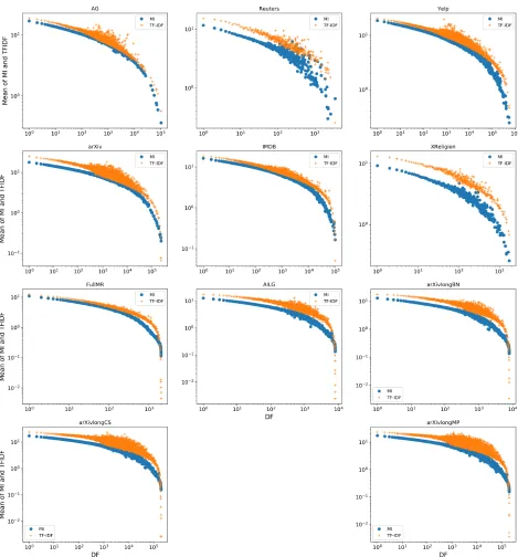
We plot how the average of TF-IDF and MI changes with the changing of df in Fig.

8. Base on the figure, we raise our theorem 3:

Theorem 3. Giving thedf as the variable, the average of TF-IDF is higher than

the average of MI when df < n₂.

We prove this theorem though the formula of TF-IDF and MI.

MIij = log2T Fij + log2 n CT Fj

+ log₂ la Di

TF-IDFij = log2T F ×log2 n dfj

+log2 n dfj

We can consider log₂ _{CT F}n

j and log2

n

dfj as a comparison group, log2T Fij and log₂T Fij ×log2

n

dfj as another group. For log₂ la

Di, empirically when we calculate the average, it is a negative number. For log₂_{CT F}n

j and log2

n

dfj, since CT Fj is the total number of term j appears in corpus and dfj is the number of documents term j appears, we can haveCT Fj ≥dfj. To check this relation, we also plot Fig. 7.

For log₂T Fij and log2T Fij×log2 dfnj, we need to consider the value of log2

n dfj. When df < n₂, means that_dfn >2, thus we have: We have:

log₂ _dfn j >1

log₂T Fij ×log2 dfnj >log2T Fij

log₂ _dfn

j ≥log2

n

CT Fj (already know)

log₂T Fij ×log2 n

dfj + log2

n

dfj >log2T Fij + log2

(37)

(38)

(39)

log₂ la

Di <0 (already know)

log₂T Fij+ log2 CT Fn j >log2T Fij + log2

n

CT Fj + log2

la

Di

log₂T Fij ×log2 n

dfj + log2

n

dfj >log2T Fij + log2

n

CT Fj + log2

la

Di

TF-IDFij >MIij

Here, our theorem 3 can be proved, and we can also observe this pattern in the

left part of Fig. 8.

3.4.3 Relationship with

T F

(a) TF-IDF and MI value under different TF values.

(b) Average of TF-IDF and MI values un-der different TF.

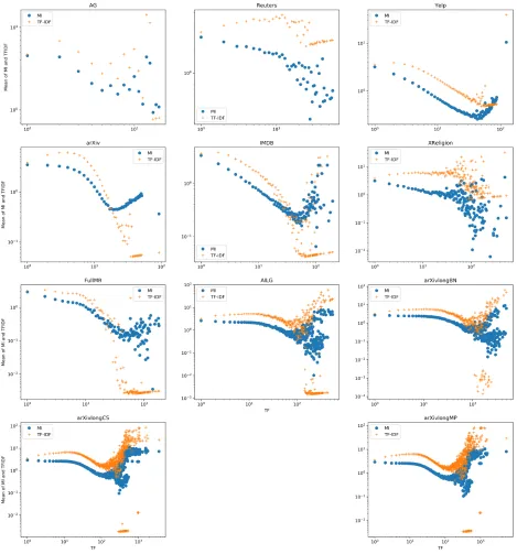
Fig. 11: MI and TFIDF values against TF on the FullMR dataset.

To understand how TF of a word is offset by its frequency in the corpus by those two

methods, we plot the MI and TFIDF values against TF in Fig 11a. As we can see,

there are too many data points, and the overall trend is obscured. Hence in panel (B),

we show the average for each TF value. From the plot, we make several observations:

1) the average of MI is smaller than the average of TFIDF overall, especially when

TF is small. 2) MI becomes bigger for larger TFs.

(40)

(41)

(42)

shape of the TF-IDF is in multiple lines. According to the formula of TF-IDF,

TF-IDFij = (log2T Fij + 1)×log2 dfnj, whendfj is fixed, since n is a constant, log2

n dfj is a constant, only T F is the variable. Thus, there is a linear relation between

TF-IDF and T F. For each dfj, there is a line reflected in the graph. Since there

are many dfj in a corpus, the shape of the TF-IDF is in multiple lines.

The shape of the MI value corresponding to theT F is discrete. According

to the formula of MI, MIij = log2T Fij+ log2CT Fn j+ log2

la

Di, whenCT F is fixed, since nis a constant, log₂ _{CT F}n

j is a constant. However, for log2

la

Di, sinceDi is the document length, Di is a variable. Thus, there does not exist a linear relation between

MI and T F, because there are two variables, Di and T F.

Base on Fig.9 and 10, we raise our hypothesis 1:

Hypothesis 1. When T F is small, the average of the TF-IDF is greater than

the average of MI, and when T F is large, the average of the relation between theses

two representation depends on thedf.

To justify the hypothesis, we need to compare the value of TFIDF and MI in two

cases.

Case 1: T F is Small

For wordswj whoseT Fij = 1,CT F could be bigger than one. According to Equation

7 and 8, the formula to calculate the MI representation can be regarded as

MI0_ij = log₂ n CT Fj

+ log₂ la Di

(11)

and the formula for the TF-IDF representation can be regarded as

TF-IDF0_ij = log₂ n dfj

(12)

From Fig. 8, we know that the average of MI is smaller than TF-IDF at most

(43)

TF-IDF0_ij >MI0_ij

log₂T Fij + 1>log2T Fij

TF-IDF0_ij ×(log₂T Fij + 1)>MIij0 ×log2T Fij ,TF-IDF0ij >1&MI

0

ij >1

From the observation of Fig. 8 we can also know that the TF-IDF0_ij >1&MI0_ij >1.

Hence, the average of MI is smaller than TF-IDF for the words with small T Fij.

Case 2: T F is large

For words with high TF, there are two situations, 1) appear in many documents (dfj

is large), 2) only appear in few documents (dfj is small).

For the words with large dfj, the dfj of these are equal or close to the n. Thus,

the _dfn

j → 1, and log2n/dfj → 0. According to the formula, the value of TF-IDF is close to 0. However, for the MI, we can transform the formula of it to:

M Iij = log2n+ log2 T Fij

CT Fj

+ log₂ la Di

(13)

We can assume that la = Di, since if we want to make M Iij close to 0, we need

to make log₂ T Fij

CT Fj → log2 1

n, means that make CT Fj close to T Fij ×n. However, it is impossible. For example on FullMR dataset, this situation happens only when

T Fij ≥ 50, and there are 2,000 documents in total in this dataset. Thus, if we want to make M Iij close to 0 for this situation, it need to have theCT Fj →50×2,000 = 100,000. However, from Fig. 7, we can find that the maximum CT F for FullMR

is 80,000, which is much less than 100,000. This restriction can also be observed on

other datasets. Thus, we can know that when both df and T F is large, the value of

M I is greater than the value of TF-IDF.

For another situation, the words with high T F only appear in a small number of

documents, which means that the dfj is small and the log2 n

(44)

greater than the df, means that log₂ n

(45)

CHAPTER 4 Neural Network Methods

Document embedding means to project the documents to a short and dense vector

representation. In TF-IDF representations, the dimension of the document

represen-tation depends on the vocabulary size, meaning that it can be sparse. Doc2Vec is the

most famous and widely used neural network method that can project the documents

into a dense vector space. Doc2Vec has two variants, and one is PV-DBOW

(Dis-tributed Bag of Words version of Paragraph Vector); the other is PV-DM (Dis(Dis-tributed

Memory version of Paragraph Vector). Doc2VecC (Doc2vec with Corruption) is the

variant of the PV-DM model; it changes the structure of PV-DM a little but improves

the performance a lot.

4.1 Doc2vec - PV-DBOW

The PV-DBOW model takes a document id as the input of the neural network to

predict the context words that are randomly sampled from the document with a fixed

window. The structure of the PV-DBOW is simple: it is just a single layer neural

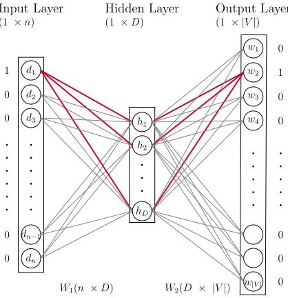
network, as shown in Fig. 12.

For each document, in each iteration of training progress, it randomly selects k

words from the document, and use the chosen words and document id di to create

k training pairs, [d1, w1],[d1, w1], ...,[d1, wk]. The training pairs are used to train the

document representation for the document di.

The input layer X is a one-hot vector, representing the document id. The length

(46)

4. NEURAL NETWORK METHODS . . . . . . . . . . . . . . Input Layer

(1 ×n)

W2(D × |V|)

W1(n ×D)

Output Layer

(1 × |V|)

Hidden Layer

(1 ×D)

d1

d2

d3

dn−1

dn h1 h2 hD w1 w4

w|V|

w3 w2 1 0 0 0 0 0 . . . . . . 0 0 0 0 1 0 . . . . .

Fig. 12: Structure of PV-DBOW

of the document with id 1, it sets 1 in the first location of the vector and 0s in other

locations.

The weight matrix W1 between the input layer and the hidden layer, also called

the document embedding matrix; this matrix is used to represent the documents.

The shape of the matrixW1 isn×d, wherenis the number of the document, anddis the dimension of the document representation set by users. There is no bias between

the input layer and the hidden layer.

Multiplying the X and W1 can get the hidden layer. Since the input layer is

just the one-hot vector for document id and W1 is the representation matrix for the

document representation matrix, the hidden layer here is the vector representation

for the training document.

The weight matrix W2 called the output matrix. The shape of W2 is d× |V|, where V is the vocabulary size. Then it uses the hidden layer to multiply with W2

can get the output layer. Finally, it applies the softmax on the output layer to get

the probability of words.

The object is to maximize the probability of the target word. Comparing the

probability of the probability generated from the output layer with the truth value

(47)

4. NEURAL NETWORK METHODS

loss to do the backpropagation to update the weight. After training, the well-trained

weight matrix W1 is the document representation matrix. The objective function of

PV-DBOW is shown in Equation 1:

J(θ) =−

n X

i=1 X wt∈di

logP(wt |di;θ) (1)

where wt are words randomly sampled from the document,n is the total number

of documents, di means document i.

Using softmax at the prediction step is expensive since for one document, it needs

V computations each iteration, here V is the vocabulary size. Thus, it can use the

Negative Sampling to reduce the time complexity. The negative sampling random

sample s negative terms (words not in document) and use the gradient ascent to

optimize the weights. Equation 2 is the probability function is used to sample the

negative terms.

P(wi) =

f(wi)3/4 Pn

j=0(f(wj)3/4)

(2)

where wi is the the word to select, f(wi) and f(wj) is the frequency of word wi

and wj appears in the corpus.

Without negative sampling, the model needs to update D× |V| weights in W2, since it needs to consider the probability of all words in the output layer. While with

negative sampling, it only needs to consider the probability of the target word and

the s negative sample. For example, if D= 100 and |V|= 10,000, without negative sampling, it needs to update 100×10,000 = 1,000,000 weights for W2; but with 5 negative samples, it only needs to update 100 ×(5 + 1) = 600 weights for W2. Complexity decreased dramatically. The objective function is changed with negative

sampling, is shown in equation 3:

Ji(θ) = X wt∈di

(logσ(vw2tdi) +

s X j∼P(w)

(48)

uments, s is number of negative samples, σ(x) = 1

1+e−x is the sigmoid function.

4.2 Doc2Vec with Corruptions

4.2.1 Doc2Vec PV-DM

Doc2vec with Corruption[5] is the variant of the Doc2Vec PV-DM model, which takes

the context words and the document ID as input and predicts the central words of

the context. Firstly, let us view the structure of the PV-DM that is shown in Fig. 13.

. . . . . . . Input Layer

W11(V × D)

W12(N × D)

Output Layer

(1 ×V)

Hidden Layer

(1 ×D)

. . . . . . . . . .

Input V ector X1

(1 × V)

Input V ector X2

(1 × N)

W2(D × V)

Fig. 13: Structure of PV-DM

It is a single layer neural network as well. In the input layer, it takes two vectors

as input; first is the vectorX1 for context words, it sets 1 to all context words and 0

to others; another is the one-hot vectorX2 for document id.

Between the input layer and the hidden layer, there are two weight matrices; the

matrixW11is the words embedding matrix, which is used to store the representations

of the words; another matrix W12 is the documents embedding matrix which stores

(49)

the context words vectors and uses X2×W12 to get the document representation for the document. Then it takes the average of the above results to get the hidden layer.

Then it uses the hidden layer to multiply the output matrix W2 to get the output

layer. Finally, it applies the softmax on the output layer to get the probability of

words.

The object is to maximize the probability of the central word. Comparing the

probability of the probability generated from the output layer with the truth value,

it can get the loss. Then it can use the loss to do the backpropagation to update

the weight. After training, the weight matrix W12 is the matrix to represent the

documents, and it can also get the weight matrixW11, which is the words embedding

matrix. Since the document representation matrix acts as a memory, which stores

the missing information here, it called the Distributed Memory version of Paragraph

Vector. The objective function of PV-DM is shown in equation 4:

J(θ) =−

n X

i=1 T−k X t=k+1

logP(wt |wt−k:wt+k;di;θ) (4)

where n is the total number of documents, k is window size, T is the length of

document di.

4.2.2 Doc2Vec with Corruption

The author of the Doc2VecC changed the structure of the PV-DM a little and

im-proved the performance and training speed a lot. In PV-DM, each document is

represented by a unique vector, but in Doc2VecC, they remove this vector. Instead,

they use the average of the words vectors in the documents. Fig. 14 shows the

structure of the Doc2VecC.

There are two vectors at the input layer as well. One is the vectorX1 for the

con-text words, which is the same as the PV-DM model. X2 is the vector that represents

the words randomly sampled from the document.

(50)

mask-out/drop-4. NEURAL NETWORK METHODS . . . . . . . Input Layer

W1(V × D)

Output Layer

(1 ×V)

Hidden Layer

(1 ×D)

. . . . . . . . . .

Input V ector X1

F or context words

(1 × V)

Input V ector X2

F or random sampled words

(1 × V)

W2(D × V)

Fig. 14: Structure of Doc2VecC

ument. Then it randomly set the values in the TF representation with the probability

q. Then it uses the 1/(1−q) to multiply with the rest values to get the new vector e

x. To summarize:

e xd=

    

0, with probability q

xd

1−q, otherwise

(5)

where _exd is the values in the new vectorxeand xd is the original values in the TF representation for the document. Finally, it times the _D1

i to the xe to get the input vector X2, Di is the document length for document i.

Between the input layer and the hidden layer, there is only one weight matrixW1,

which is the words representation matrix. X1×W1gives the sum of the words vectors of the context words, X2×W1 gives the average of the sum of the words vectors for words random sampled, and sum the above two results can get the hidden layer. The

following structures are the same as the PV-DM model, times the hidden layer with

the output matrix W2 to get the output layer and use the softmax to calculate the

probability and compare with the truth, get the loss to make gradient descent. The

(51)

After the training, it can give a well-train words representation matrix W1, and

the document is represented by the average of the embeddings of the words in the

documents like equation 6 shows.

Vi = 1 Di

X w∈di

vw (6)

where Vi is the representation for document di, Di is the document length for di

(52)

CHAPTER 5 Experiments

5.1 Datasets

There are three aspects of the dataset considered as the main features when we collect

the data. One is the size of the dataset since we want to figure out whether the size

of data plays an essential role in the vectorized step. Another feature is the average

length. The third feature is the vocabulary size of the data, which can also influence

the performance of the vectorizing and classification results. The detailed information

of all the datasets used in this thesis is showing in Table 10.

Dataset # of Documents # of classes Vocab Size Average Length CV of Length CV of CTF

Datasets from Others

AG’s news 127,600 4 63,152 36 0.28 18.22 Reuters 4,000 2 15,907 91 1.07 11.09 Yelp Review Polarity 598,000 2 221,477 126 0.92 40.94 IMDB 100,000 2 138,514 225 0.75 34.27 20 News Group 1,985 2 25,073 235 2.57 13.39 Full Movie Review 2,000 2 38,880 627 0.44 17.76 arXiv CS vs., non-CS 240,000 2 163,543 145 0.43 40.32 Long arXiv CS vs., non-CS 200,000 2 1,606,482 1,100 0.66 117.50

Math vs., Physics 200,000 2 1,412,812 1,071 0.64 120.02 Business vs., not 8,000 2 157,844 1,081 0.60 39.90 AI vs., Machine Learning 8,000 2 145,001 1,085 0.64 34.13

(53)

5. EXPERIMENTS

5.1.1 Data Description

AG’s News

The AG(Antonio Gulli)’s corpus of news articles contains millions of news. It collects

news from more than 2000 news sources. Each data consists of a title and a short

description of the news. In our thesis, we use the largest four groups of news: Business,

Sports, World, and Sci/Tech. The dataset contains 127,600 documents, and they are

divided equally into four groups (31900 documents each class). This dataset is used

in [24][6].

Reuters News

Reuters News is a publically available version of the well-known Reuters-21578

“Mod” corpus for text categorization. It has been used in publications like [23].

Apte-Mod is a collection of 10,788 documents from the Reuters financial newswire service.

There are 90 categories in the corpus. In our experiments, we randomly select 4,000

documents from the largest two categories (‘earn’ and ‘acq’) equally.

Yelp Review Polarity

The Yelp Review dataset[24] is an open-source dataset provided by Yelp for NLP

training. The data we use in this thesis contains 598,000 reviews, and the dataset is

divided into two groups, positive and negative equally. This dataset is used in [24].

IMDB

The IMDB dataset[11]1 _{is the famous and common dataset for the sentiment analysis}

and text classification. It contains 10,000 movie reviews that are taken from IMDB

(Internet Movie Database). The dataset is divided into three sub-dataset: 25,000

training data, 25,000 testing data, and 50,000 unlabeled data. In our experiments,

we mix the training and test datasets and used the 10-fold cross-validation. For

(54)

5. EXPERIMENTS

embeddings. There are only two classes in this dataset, positive and negative.

20 NewsGroups

The 20 Newsgroups dataset2 _{is a collection of approximately 20,000 newsgroup}

docu-ments, partitioned (nearly) evenly across 20 different newsgroups. In our experiment,

since we want to conduct a dataset with the long average length, we only use two

newsgroups to do the classification task, which is “comp.windows.x” group (988

doc-uments) and “soc.religion.christian” group (997 docdoc-uments), we denote this dataset

as “XReligion”.

Full Movie Review

The Full Movie Review dataset[15] consists of 2000 full-length movie reviews. The

dataset is divided into two groups, positive and negative equally. Full Movie Review

is the dataset with the highest average length in our experiments.

arXiv

ArXiv is an open-source academic papers library that was started in 1991 and

main-tained by Cornell University Library. It collected millions of academic papers in areas

such as physics, mathematics, computer science, statistics, etc. The official website

provides access to download the full-text data (pdf format and LaTex format) and

the metadata. For the metadata, we can use the provided API to get the paper

ID, title, abstract, and author. We used the API to collect the metadata of papers

from 1990-01-01 to 2018-08-31. After removing the duplicates, there are 1,402,977

papers in total. Including 151,321 Computer Science papers, 314,003 Math papers,

19,615 Statistics papers, 15,285 Quantitative Biology papers, 59,65 Quantitative

Fi-nance papers, 278 Electrical Engineering and Systems Science papers and only 1,696

Economics papers, and the rest are 894,814 Physics papers. All the labels of the

arXiv documents are labelled by the author. In our experiments, directly do the

(55)

5. EXPERIMENTS

classification experiment on the entire data is too time-consuming, especially we are

running 10-fold cross-validation. To reduce the size of the data, we randomly select

120,000 docs from both the Computer Science category and non-CS categories, we

make them balanced. We denoted this dataset as “arXiv”; the papers in this dataset

only contain the title and abstract.

We also downloaded the full-text data in LaTeX format. Moreover, we had

ex-tracted the paper ID and the introduction subsection of papers. Then we merged the

introduction subsections and the title and abstracts we previous had according to the

paper ID and got the Long arXiv data set. In our experiment, we tested on a few

com-binations of the classes; all comcom-binations are balanced with docs sampled randomly.

Those combinations are arXivLongCS (CS vs. non-CS), arXivLongBN (Business vs.

non-Business), arXivLongMP (Math vs. Physics), AILG (AI vs. Machine Learning3_).

5.1.2 Observation of Datasets

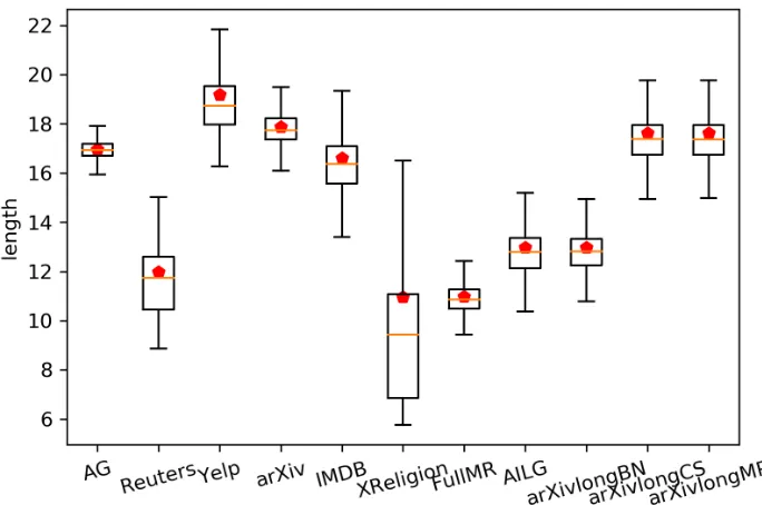
Fig. 15 shows the distribution of the document lengths for every dataset, the

x-axis is the lengths of the documents, and the y-x-axis is the percentage of the length

occurrence. Fig. 16 and 17 show the distribution of the CTF. We also list the

coefficient of variation of the length and CTF of all datasets in Table 10. The reason

for studying the distribution of CTF is that the CTF plays an important role in our

MI representation method. From Fig. 17 and 16, we can observe that all the data

follow Zipf’s Law. Since the CTF for different words can be different, the coefficient

of variation of CTF should be huge can related to the vocabulary size. Table 10 shows

that the CTF of all datasets follows the above pattern. From Fig. 15 and Table 10,

we can know that all the distribution of the length follows or closes to the normal

distribution, besides the Reuters and XReligion. The coefficient of variation of the

length distribution of XReligion is significantly large; it has many documents that

only include few words and many documents with thousands of words.

3_{In the official description, the AI labels cover all areas of AI except Vision, Robotics, Machine}

(56)

5. EXPERIMENTS

(57)

5. EXPERIMENTS

(58)

5. EXPERIMENTS

(59)

5. EXPERIMENTS

5.2 Experimental Setup

In our experiments, we use the standard 10 fold cross-validation to evaluate the

performance. N fold is the dataset splitting technique. For example, if we use

10-fold, we divide the dataset into 10 parts at the beginning. First, we use [0,₁₀1] part

of the data to be the test set, and use [₁₀1 ,10₁₀] part of the data to train the classifier.

And in the second iteration, use [₁₀1,₁₀2] part of the data to be the test set, and use

[0,₁₀1 ]S [₁₀2 ,10

10] part of the data to train the classifier. Iterate 10 times until all parts of the data have been tested and assigned a predicted class label. 10-fold

cross-validation is time-consuming, but the result is reliable. In our experiments, we use

ten 10-fold cross-validations to ensure the accuracy of the result.

Based on the results of the cross-validation, TP(True Positive), TN(True

Nega-tive), FP(False PosiNega-tive), FN(False Negative) are obtained. Thus we can evaluate the

results according to the F1 score as follows:

P recision= T P T P +F N

Recall= T P

T P +F P (1)

F1 = 2×

P recision×Recall P recision+Recall

The above formula is for the F1 for the binary classification problem, but we have

the multi-classes in one of our datasets, we can use themacro-F1[18] to evaluate the

result. The formula for macro-F1 is shown as bellow.

Macro-Precision = P recision1+...+P recisionn n

Macro-Recall = Recall1+...+Recalln

n (2)

Macro-F1 = 2× Macro-Precision×Macro-Recall

(60)

5. EXPERIMENTS

Datasets TF-IDF MI

AG’s news 0.8831 0.8804

Reuters 0.9823 0.9814

Yelp Review 0.9165 0.9099

arXiv 0.9304 0.9343

IMDB 0.8864 0.8846

XReligion 0.9700 0.9727

Full Movie Review 0.8662 0.8834

AILG 0.8803 0.8849

arXivLongBN 0.9822 0.9819

arXivLongMP 0.9733 0.9747

arXivLongCS 0.9618 0.9638

Table 11: Macro-F1 score of MI representation and TF-IDF representation on all datasets used in our thesis (Higher is better). Bold means better in that datasets.

5.3 Comparison of MI and TF-IDF

Firstly, we evaluated the performance of our MI representation against the TF-IDF.

Table 11 shows the macro-F1 score of two methods. Fig. 18 shows the

improve-ment ratio of the MI representation comparing to the TF-IDF representation; the

formula for improvement ratio is shown below. Here F1a is the macro-F1 of the MI

representation, and F1b is the macro-F1 of the TF-IDF representation.

Improvement Ratio = F1a−F1b F1b

×100 (3)

The order of the datasets in the above graph is sorted by average length. Fig. 18

shows that MI outperforms TF-IDF when the average length of the datasets is long.

The improvement ratio is especially high for the FullMR dataset. We also make a

significant test on the results to check the p-value, since we want to make sure the